Galaxy Cluster Correlation Function to $z\sim 1.5$ in the IRAC Shallow Cluster Survey

Abstract

We present the galaxy cluster autocorrelation function of 277 galaxy cluster candidates with $0.25\leq z\leq 1.5$ in a 7 deg² area of the IRAC Shallow Cluster Survey. We find strong clustering throughout our galaxy cluster sample, as expected for these massive structures. Specifically, at $\left<z\right>=0.5$ we find a correlation length of $r_{0}=17.40^{+3.98}_{-3.10}$ $h^{-1}$ Mpc, in excellent agreement with the Las Campanas Distant Cluster Survey, the only other non–local measurement. At higher redshift, $\left<z\right>=1$, we find that strong clustering persists, with a correlation length of $r_{0}=19.14^{+5.65}_{-4.56}$ $h^{-1}$ Mpc. A comparison with high resolution cosmological simulations indicates these are clusters with halo masses of $\sim 10^{14}M_{\odot}$, a result supported by estimates of dynamical mass for a subset of the sample. In a stable clustering picture, these clusters will evolve into massive ($10^{15}M_{\odot}$) clusters by the present day.

1. Introduction

The clustering amplitude of massive galaxy clusters, and in particular its dependence on richness or cluster mass, is a strong function of the underlying cosmology. Recent theoretical work (e.g., Majumdar and Mohr, 2003; Younger et al., 2006) has demonstrated how cluster surveys can be “self–calibrated,” providing precise simultaneous constraints on both the cosmology and cluster evolution models. Given redshift and approximate mass information for each cluster, reliable cosmological parameter estimation is feasible even in the presence of significant, and potentially unknown, evolution in cluster physical parameters (e.g., Gladders et al., 2007). The ultimate goal of these cosmological studies, a measurement of the equation of state of dark energy with an accuracy competitive with SNe Ia methods, also requires knowledge of the cluster power spectrum or autocorrelation function (Majumdar and Mohr, 2004; Wang et al., 2004). Such extensive sample characterization naturally emerges from mid–infrared selected photometric redshift cluster surveys like the IRAC Shallow Cluster Survey (ISCS; Eisenhardt et al., 2007, hereafter E07).

Previous studies (e.g., Bahcall et al., 2003, and references therein) have produced largely local ($z\lesssim 0.3$) galaxy cluster clustering measurements with limited baselines for evolutionary studies. The ISCS provides the opportunity to address these issues in one of the largest statistical samples of high redshift clusters to date. In this Letter we present the first measurement of the galaxy cluster autocorrelation function extending over more than half the cosmic age of the Universe. Such measurements also allow evolutionary connections between galaxy clusters and high redshift, highly clustered galaxy populations to be explored.

We use a concordance cosmology throughout, with $\Omega_{M}=0.3$, $\Omega_{\Lambda}=0.7$, and $H_{0}=70$ km s${}^{-1}\!$ Mpc^-1. For consistency with previous studies we report distances, including correlation lengths, in units of comoving $h^{-1}$ Mpc, with $H_{0}=100\,h$ km s^-1 Mpc^-1.

2. IRAC Shallow Cluster Survey

The ISCS is a sample of 335 galaxy clusters spanning $0.1<z<2$ in the IRAC Shallow Survey (ISS, Eisenhardt et al., 2004) area of the NOAO Deep-Wide Field Survey (NDWFS, Jannuzi and Dey 1999; Jannuzi et al. in prep) in Boötes. The clusters are selected using a wavelet detection algorithm which identifies peaks in cluster probability density maps constructed from accurate photometric redshift probability functions for 175,431 galaxies brighter than 13.3$\mu$Jy at 4.5$\mu$m in a 7.25 deg² region (Brodwin et al. 2006, hereafter B06; E07). The galaxy photometric redshifts, which are key to the cluster–finding algorithm, are derived from the joint ISS, NDWFS (DR3) and FLAMEX (Elston et al., 2006) data sets.

The AGES survey (Kochanek et al. in prep) in Boötes provides spectroscopic confirmation for dozens of clusters at $z\leq 0.5$ (E07). At higher redshift, a multi–year Keck spectroscopic campaign has to date confirmed 10 $z>1$ clusters (Stanford et al. 2005; Elston et al. 2006; B06; E07).

Extensive masking, described in B06, is implemented to reject areas suffering from remnant cosmetic artifacts or data quality issues which could affect the robustness of the clustering measurements. The final unmasked area is 7.00 deg² and contains 320 of the 335 galaxy clusters in the full ISCS, of which 277 are within the redshift range ($0.25\leq z\leq 1.5$) considered in this Letter.

3. Galaxy Cluster Autocorrelation Measurements

3.1. Angular Correlation Function in Redshift Slices

The redshift distribution of galaxy clusters is presented in Figure 1. A fit of the form $N(z)\propto(z/z_{0})^{\alpha}\exp{(-(z/z_{0})^{\beta})}$, with $\alpha=1.5$, $\beta=1.7$ and $z_{0}=0.7$, is overplotted. Cosmological studies with this observed redshift distribution must await a detailed characterization of the survey selection function, to be presented in a forthcoming paper. Galaxy clusters are split into two similarly populated redshift bins, $0.25\leq z\leq 0.75$ (136 clusters) and $0.75<z\leq 1.5$ (141 clusters), using the best available redshift information (i.e., spectroscopic redshifts where available, photometric redshifts otherwise). These bins span the range where the accuracy, $\sigma_{z}=0.06(1+z)$, and reliability of the galaxy photometric redshifts have been demonstrated (B06; see also Brown et al. 2007).

Figure 1.— Observed redshift distribution of galaxy clusters in the ISCS. The dashed lines illustrate the two redshift bins considered here, $0.25\leq z\leq 0.75$ and $0.75<z\leq 1.5$, containing 277 clusters between them. The curve is a fit to the distribution and is used in the Limber deprojection. This distribution should not be used for quantifying number density evolution without careful inclusion of selection biases.

The angular correlation function (ACF) is parametrized here as a simple power law,

$$\omega(\theta)=A_{\omega}\theta^{-\delta}.$$ (1)

This can be deprojected (Limber, 1954) to yield a measurement of the real–space correlation length, $r_{0}(z)$, over the redshift range spanned by the 2–D sample,

$$r_{0}^{\gamma}(z_{\mbox{\scriptsize eff}})=A_{\omega}\left[\frac{H_{0}H_{\gamma}}{c}\,\frac{\int_{z_{1}}^{z_{2}}N^{2}(z)\,[x(z)]^{1-\gamma}\,E(z)\,dz}{[\int_{z_{1}}^{z_{2}}N(z)\,dz]^{2}}\right]^{-1},$$ (2)

where

$$z_{\mbox{\scriptsize eff}}=\frac{\int_{z_{1}}^{z_{2}}z\,N^{2}(z)\,[x(z)]^{1-\gamma}\,E(z)\,dz}{\int_{z_{1}}^{z_{2}}N^{2}(z)\,[x(z)]^{1-\gamma}\,E(z)\,dz},$$ (3)

$\gamma\equiv 1+\delta$, $H_{\gamma}=\Gamma(1/2)\,\,\Gamma[(\gamma-1)/2]/\Gamma(\gamma/2)$, $N(z)$ is the redshift distribution, and $E(z)$ and $x(z)$ describe the evolution of the Hubble parameter and the comoving radial distance, respectively (e.g., Hogg, 1999). Since the cluster redshift uncertainties are much smaller than the width of our redshift bins (E07), they have little impact on the redshift distribution and the modeling of the spatial correlation function.

3.2. Results

We calculate the ACF using both the Landy and Szalay (1993) and Hamilton (1993) estimators using 500,000 randoms to ensure a robust Monte Carlo integration. The results are nearly identical with both estimators and we report the results obtained with the latter. Two independent fitting techniques are applied to the data. The standard frequentist (or classical) approach is used to simultaneously fit the slope, and, through the use of the relativistic Limber equation, the correlation length, $r_{0}$. In calculating these correlation lengths we have adopted the $N(z)$ parametrization shown in Figure 1. A Bayesian technique is also employed to directly determine the correlation lengths, marginalizing over the slope, $\delta$, subject to the weak prior that it is in the range $0.2\leq\delta\leq 1.8$. This method is desirable since, despite the large number of clusters, it is difficult to simultaneously constrain both amplitude and slope. Figure 2 shows both the frequentist fits and the Bayesian likelihood functions in $r_{0}$.

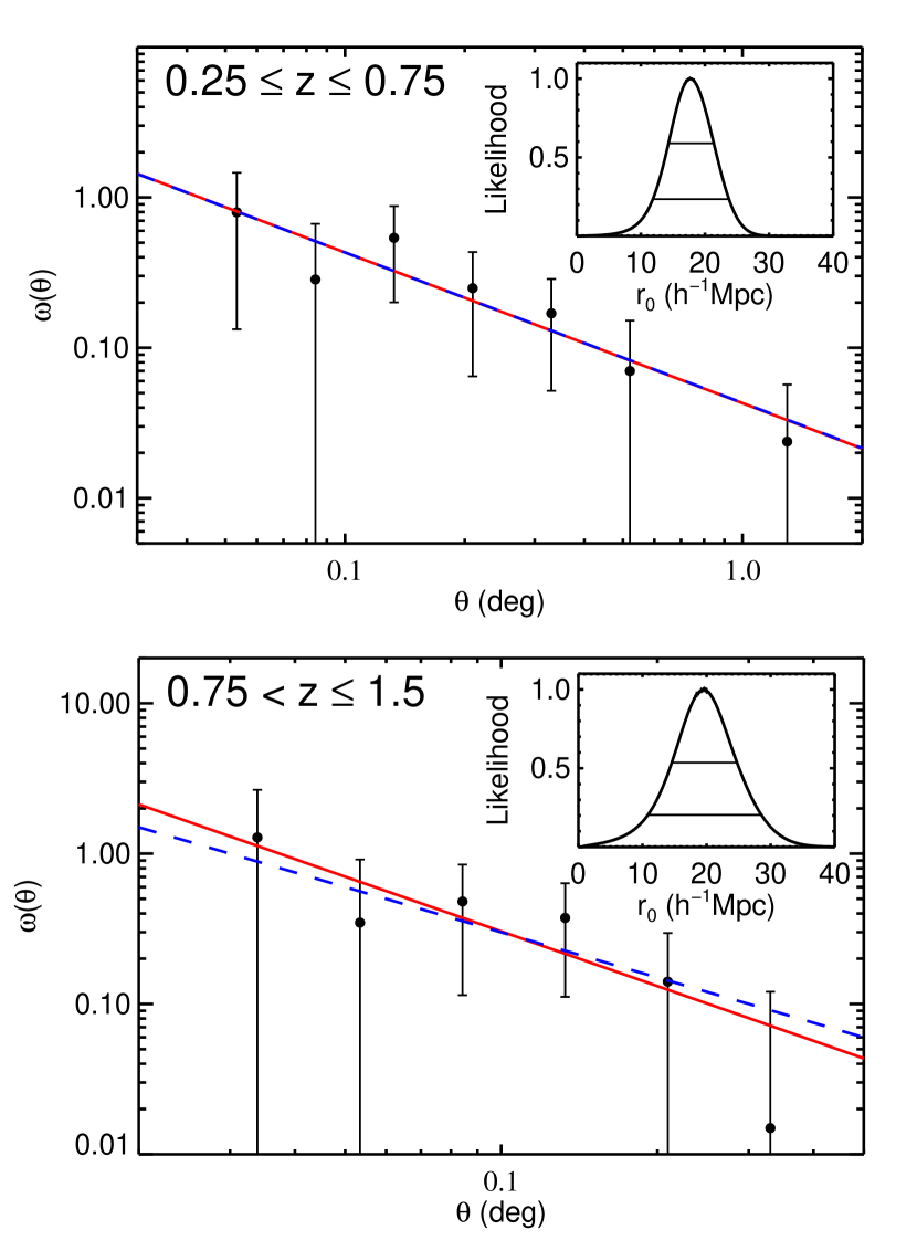
Figure 2.— Angular correlation functions in redshift bins at $0.25\leq z\leq 0.75$ (top) and $0.75<z\leq 1.5$ (bottom). The error bars are estimated via bootstrap resampling. The red solid lines show the best–fit ACFs, with corresponding slopes listed in Table 1. The blue dashed lines show the fits with a fixed slope ($\delta=1.0$). Marginalizing over the slope produces the likelihood functions in $r_{0}$ presented in the insets. The 68% and 90% confidence intervals are shown.

In this highly clustered population, sample (or cosmic) variance dominates over simple Poisson errors. We therefore calculate the error bars using 100 bootstrap resamplings with replacement. To test for possible systematics across the field we divided the field into halves, once north–south and once east–west, and for each subfield we computed the ACF. The results for all half–fields agree within 1 $\sigma$, indicating that we are not adversely affected by an unidentified bias in the spatial selection function.

Bootstrap simulations of the cluster detection process indicate that the spurious fraction is less than 10% at all redshifts (E07), and spectroscopic observations indicate it is likely much lower. Conservatively assuming 5–10% of the sample is indeed spurious, and that these are uncorrelated, then at most we are underestimating the clustering by $\approx$ 11–23%.

In this work we adopt the $r_{0}$ values from the Bayesian fits, though the fits from both methods, presented in Table 1, are completely consistent. The correlation amplitude in our low redshift bin at $z\approx 0.5$ is in excellent agreement with the only other measurement at this redshift (Gonzalez et al., 2002). Our high redshift measurement, at $z\approx 1$, is the first to probe structure on the largest scales in the first half of Universe.

The space densities for these samples and the mean intercluster distances, $d_{c}$, are also presented in Table 1. The relationship between clustering amplitude and $d_{c}$ predicted in a concordance cosmology, and observed in practice (Bahcall et al., 2003, and references therein), is only weakly dependent on redshift. As shown in Figure 3, the ISCS samples are quite consistent with the LCDM predictions between $0<z<1.5$ (hashed region) from Younger et al. (2005).

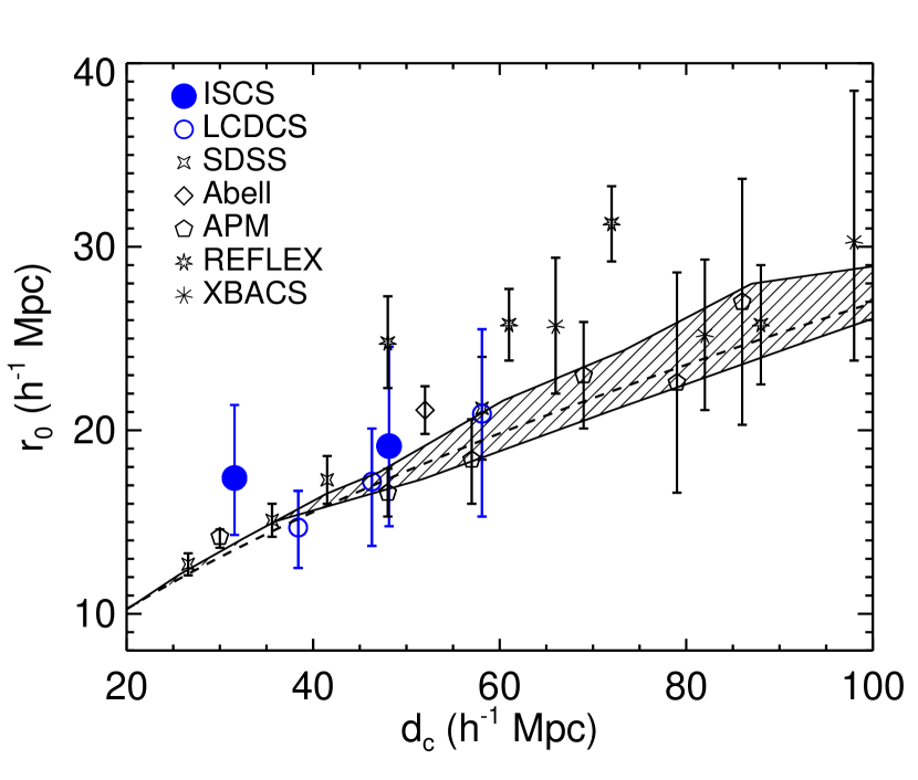
Figure 3.— Plot of $r_{0}$ vs. $d_{c}$ for the present sample, along with several measurements taken from the compilation of Bahcall et al. (2003). Our results (filled blue circles) are consistent with LCDM predictions between $0<z<1.5$ (hashed region), with the parametrization of Younger et al. (2005, dashed line), as well as with the most distant measurement prior to the present one, the LCDCS at $z\sim 0.5$ (open blue circles). Data are from Gonzalez et al. (2002); Abadi et al. (1998); Croft et al. (1997); Peacock and West (1992); Bahcall and Soneira (1983); Collins et al. (2000); Lee and Park (1999).

Table 1Amplitude of Correlations for ISCS Clusters

$\Delta z$	$z_{\mbox{\small eff}}$	$N$	$\log A_{\omega}$	$r_{0}$	$\delta$	$r_{0}$	$\bar{n}$	$d_{c}$
				($h^{-1}$ Mpc)		($h^{-1}$ Mpc)	($10^{-6}$ $h^{3}$ Mpc-3)	($h^{-1}$ Mpc)
0.25 – 0.75	0.53	136	$-1.37\pm^{0.18}_{0.31}$	$18.70\pm^{4.31}_{5.66}$	$1.00\pm^{0.29}_{0.46}$	$17.40\pm^{3.98}_{3.10}$	$31.8\pm 2.7$	$31.6\pm 0.9$
0.75 – 1.50	0.97	141	$-1.73\pm^{0.52}_{0.23}$	$18.64\pm^{5.18}_{7.66}$	$1.21\pm^{0.29}_{0.94}$	$19.14\pm^{5.65}_{4.56}$	$8.96\pm 0.76$	$48.1\pm 1.4$

4. Discussion

Figure 4.— Comoving correlation lengths for the ISCS clusters, along with other cluster samples at lower redshift (offset slightly in z for clarity) and highly clustered galaxy samples at higher redshifts (see the text for a full description and references). Two evolutionary models are overplotted, including the Fry (1996) biased structure formation model (shaded region and dotted lines for $z_{\mbox{\scriptsize eff}}=0.53$ and $0.97$, respectively), and a simple stable clustering model (dashed lines).

A key theoretically predictable cluster observable is the correlation function as a function of halo mass. In simulations the halo mass, $M_{\mbox{\scriptsize 200}}$, is defined as the mass inside the radius at which the mean overdensity is 200 times the critical density. We compare our clustering results with the Younger et al. (2005) analysis of the Hopkins et al. (2005) high–resolution cosmological simulation, which had a 1500 $h^{-1}$ Mpc box length, an individual particle mass of $1.8\times 10^{11}\hbox{$M_{\odot}$}$, and a power spectrum normalization of $\sigma_{8}=0.84$. We infer that the ISCS cluster sample has average $\log[M_{\mbox{\scriptsize 200}}/M_{\odot}]$ masses of $\sim 13.9^{+0.3}_{-0.2}$ and $\sim 13.8^{+0.2}_{-0.3}$ at $z_{\mbox{\scriptsize eff}}=0.53$ and $0.97$, respectively. Direct dynamical masses for the 10 $z>1$ clusters presented in E07 yield a largely consistent distribution of masses (Gonzalez et al. in prep).

The observed constancy of $r_{0}$ for massive galaxy clusters out to $z=1$ is a robust confirmation of a key prediction from numerical simulations, reflecting the relative constancy of the mass hierarchy of clusters with redshift (Younger et al., 2005). That is, the N most massive clusters at one epoch roughly correspond to the N most massive clusters at a later epoch, and therefore have similar clustering.

In Figure 4 we plot a compilation of recent clustering amplitudes for various cluster surveys, as well as for highly clustered galaxy populations, including FRII radio galaxies (Overzier et al., 2003), EROs (Brown et al., 2005; Daddi et al., 2004, 2001), ULIRGs (Farrah et al., 2006; Magliocchetti et al., 2007), and SMGs (Blain et al., 2004). Since optically–selected QSOs are more modestly clustered (Porciani et al., 2004; Croom et al., 2005; Myers et al., 2006; Coil et al., 2007), and therefore reside in considerably less massive halos ($\sim 10^{12}-10^{13}M_{\odot}$) than the ISCS clusters, they are not included in Figure 4.

Following Moustakas and Somerville (2002), we overplot the halo conserving model of Fry (1996) normalized to our two measurements in order to explore possible evolutionary connections with structures at other redshifts. The shaded area (dotted lines) shows the 1 $\sigma$ region for the $z_{\mbox{\scriptsize eff}}=0.53$ ($0.97$) measurement. In this model, representative of a class of merger-free biased structure formation models, the ISCS clusters will evolve into typical present–day massive clusters, such as those in the SDSS, APM or Abell surveys. In the stable–clustering picture, in which clustering is fixed in physical coordinates (Groth and Peebles, 1977, dashed lines), the $z_{\mbox{\scriptsize eff}}=0.97$ ISCS clusters grow into the most massive clusters in the local Universe, typically identified in X–ray surveys.

Most of the plotted high redshift galaxy clustering measurements are rather uncertain due to both small number statistics and poorly known redshift distributions. Mindful of this caveat, we observe that FRII radio galaxies, some ERO samples, and $z\sim 2$ ULIRGs have clustering consistent with that seen in the ISCS clusters in either model. Clearly these populations trace very massive halos ($\gtrsim 10^{13}M_{\odot}$). As a caution against overinterpretation, however, we note that only ULIRGs have space densities similar to the present cluster samples, a prerequisite for drawing evolutionary connections from these particular models. Thus the present work offers a measure of support for recent studies (e.g., Magliocchetti et al., 2007) indicating that ULIRGs may be associated with, or progenitors of, groups or low–mass clusters.

5. Conclusions

By deprojecting the angular correlation function measured in redshift bins spanning $z=0.25$ to $z=1.5$, we have determined the real–space clustering amplitudes for ISCS clusters at $\left<z\right>=0.53$ and $\left<z\right>=0.97$ to be $r_{0}=17.40^{+3.98}_{-3.10}$ and $r_{0}=19.14^{+5.65}_{-4.56}$ $h^{-1}$ Mpc, respectively. These measurements are consistent with the relation between correlation amplitude and mean intercluster distance predicted by LCDM. The ISCS clusters have total masses exceeding $10^{14}M_{\odot}$ and will evolve into very massive clusters by the present day.

References

- Abadi et al. (1998) Abadi, M. G., Lambas, D. G., and Muriel, H. 1998, ApJ 507, 526
- Bahcall et al. (2003) Bahcall, N. A., Dong, F., Hao, L., Bode, P., Annis, J., Gunn, J. E., and Schneider, D. P. 2003, ApJ, 599, 814
- Bahcall and Soneira (1983) Bahcall, N. A. and Soneira, R. M. 1983, ApJ, 270, 20
- Blain et al. (2004) Blain, A. W., Chapman, S. C., Smail, I., and Ivison, R. 2004, ApJ. 611, 725
- Brodwin et al. (2006) Brodwin, M., et al. 2006, ApJ, 651, 791
- Brown et al. (2007) Brown, M. J. I., Dey, A., Jannuzi, B. T., Brand, K., Benson, A. J., Brodwin, M., Croton, D. J., and Eisenhardt, P. R. 2007, ApJ, 654, 858
- Brown et al. (2005) Brown, M. J. I., Jannuzi, B. T., Dey, A., and Tiede, G. P. 2005, ApJ, 621, 41
- Coil et al. (2007) Coil, A. L., Hennawi, J. F., Newman, J. A., Cooper, M. C., and Davis, M. 2007, ApJ, 654, 115
- Collins et al. (2000) Collins, C. A., et al. 2000, MNRAS, 319, 939
- Croft et al. (1997) Croft, R. A. C., Dalton, G. B., Efstathiou, G., Sutherland, W. J., and Maddox, S. J. 1997, MNRAS, 291, 305
- Croom et al. (2005) Croom, S. M., et al. 2005, MNRAS, 356, 415
- Daddi et al. (2001) Daddi, E., Broadhurst, T., Zamorani, G., Cimatti, A., Röttgering, H., and Renzini, A. 2001, A&A, 376, 825
- Daddi et al. (2004) Daddi, E., et al. 2004, ApJ, 600, L127
- Eisenhardt et al. (2007) Eisenhardt, P. R., et al. 2007, ApJ, submitted
- Eisenhardt et al. (2004) Eisenhardt, P. R., et al. 2004, ApJS, 154, 48
- Elston et al. (2006) Elston, R. J., et al. 2006, ApJ, 639, 816
- Farrah et al. (2006) Farrah, D., et al. 2006, ApJ, 641, L17
- Fry (1996) Fry, J. N. 1996, ApJ, 461, L65
- Gladders et al. (2007) Gladders, M. D., Yee, H. K. C., Majumdar, S., Barrientos, L. F., Hoekstra, H., Hall, P. B., and Infante, L. 2007, ApJ 655, 128
- Gonzalez et al. (2002) Gonzalez, A. H., Zaritsky, D., and Wechsler, R. H. 2002, ApJ, 571, 129
- Groth and Peebles (1977) Groth, E. J. and Peebles, P. J. E. 1977, ApJ, 217, 385
- Hamilton (1993) Hamilton, A. J. S. 1993, ApJ, 417, 19
- Hogg (1999) Hogg, D. W. 1999, astro-ph/9905116
- Hopkins et al. (2005) Hopkins, P. F., Bahcall, N. A., and Bode, P. 2005, ApJ, 618, 1
- Jannuzi and Dey (1999) Jannuzi, B. T. and Dey, A. 1999, in ASP Conf. Ser. 191 — Photometric Redshifts and the Detection of High Redshift Galaxies, p. 111
- Landy and Szalay (1993) Landy, S. D. and Szalay, A. S. 1993, ApJ, 412, 64
- Lee and Park (1999) Lee, S. and Park, C. 1999, J. Korean Astron.Soc. 32, 1
- Limber (1954) Limber, D. N. 1954, ApJ, 119, 655
- Magliocchetti et al. (2007) Magliocchetti, M., Silva, L., Lapi, A., de Zotti, G., Granato, G. L., Fadda, D., and Danese, L. 2007, MNRAS, 375, 1121
- Majumdar and Mohr (2003) Majumdar, S. and Mohr, J. J. 2003, ApJ, 585, 603
- Majumdar and Mohr (2004) Majumdar, S. and Mohr, J. J. 2004, ApJ, 613, 41
- Moustakas and Somerville (2002) Moustakas, L. A. and Somerville, R. S. 2002, ApJ, 577, 1
- Myers et al. (2006) Myers, A. D., et al. 2006, ApJ, 638, 622
- Overzier et al. (2003) Overzier, R. A., Röttgering, H. J. A., Rengelink, R. B., and Wilman, R. J. 2003, A&A, 405, 53
- Peacock and West (1992) Peacock, J. A. and West, M. J. 1992, MNRAS, 259, 494
- Porciani et al. (2004) Porciani, C., Magliocchetti, M., and Norberg, P. 2004, MNRAS, 355, 1010
- Stanford et al. (2005) Stanford, S. A., et al. 2005, ApJ, 634, L129
- Wang et al. (2004) Wang, S., Khoury, J., Haiman, Z., and May, M. 2004, Phys. Rev. D, 70, 123008
- Younger et al. (2005) Younger, J. D., Bahcall, N. A., and Bode, P. 2005, ApJ, 622, 1
- Younger et al. (2006) Younger, J. D., Haiman, Z., Bryan, G. L., and Wang, S. 2006, ApJ, 653, 27