Forbidden ordinal patterns in higher dimensional dynamics

Abstract

Forbidden ordinal patterns are ordinal patterns (or ‘rank blocks’) that cannot appear in the orbits generated by a map taking values on a linearly ordered space, in which case we say that the map has forbidden patterns. Once a map has a forbidden pattern of a given length $L_{0}$, it has forbidden patterns of any length $L\geq L_{0}$ and their number grows superexponentially with $L$. Using recent results on topological permutation entropy, we study in this paper the existence and some basic properties of forbidden ordinal patterns for self maps on $n$-dimensional intervals. Our most applicable conclusion is that expansive interval maps with finite topological entropy have necessarily forbidden patterns, although we conjecture that this is also the case under more general conditions. The theoretical results are nicely illustrated for $n=2$ both using the naive counting estimator for forbidden patterns and Chao’s estimator for the number of classes in a population. The robustness of forbidden ordinal patterns against observational white noise is also illustrated.

PACS: 02.50.Ey, 05.45.Vx, 89.70.+c

1 Introduction

Ordinal patterns of length $L$ describe the relations of ‘smaller’ or ‘larger’ among $L$ consecutive points of a deterministically or randomly generated sequence in a linearly ordered space. Ordinal patterns are the main ingredient of permutation entropy, a concept introduced both in metric and topological versions by Bandt, Keller and Pompe [6], that were shown to coincide with their standard counterparts for piecewise monotone one-dimensional interval maps. Later on, the concepts of metric and topological permutation entropies were generalized to $n$-dimensional interval maps in [1] and [2], respectively, while preserving the main results of [6] although under different assumptions: ergodicity for the metric entropy and expansiveness for the topological entropy. Both generalizations parallel Kolmogorov’s construction of entropy in dynamical systems in that they coarse-grain the state space with partitions, apply the corresponding definition of entropy to the resulting symbolic dynamics and, lastly, take ever finer partitions. But this time the partitions used are product, uniform partitions (the original, one-dimensional versions even dispense thoroughly with partitions), making possible, albeit computationally demanding, the numerical estimation of metric and topological entropy. Moreover, ordinal patterns allow a unified and conceptually simple approach both to metric and topological entropy, at variance with the standard approach.

In this paper, that can be considered a second part of [2], we deal only with the topological permutation entropy. Having shown in [2] that this concept converges to topological entropy for $n$-dimensional expansive interval maps and illustrated how it can be used as estimator, we focus our attention now on some interesting consequences of order in dynamical systems.

First of all, it turns out that the orbits of continuous, $n$-dimensional interval maps with finite topological permutation entropy have always forbidden patterns, i.e., ordinal patterns that cannot occur in the orbits of the map, in contrast with (unconstrained) random time series, in which any ordinal patterns appears with probability $1$. As a more practical result, it follows that the same happens to expansive maps with finite topological entropy. Furthermore, forbidden patterns proliferate superexponentially with length, the exact details being controlled by the topological permutation entropy. The existence and growth rate of forbidden patterns was already considered in [3, 4, 5] but in a rather restrictive setting, namely, for piecewise monotone maps on one-dimensional intervals only (i.e., using the original definition of topological permutation entropy and results of [6]). In the present paper, we go higher dimensional by using the definitions and results of [2].

Secondly, forbidden patterns are, in general, not invariant under isomorphism (or conjugacy) between dynamical systems unless the isomorphism is order-preserving, i.e., it is an order-isomophism. This allows to further subdivide isomorphic systems according to their forbidden patterns, thus opening the door to more restrictive definitions of equivalence among maps of $n$-dimensional intervals.

Last but not least, forbidden patterns are robust against observational noise on account of being defined by inequalities. Robustness was shown in [4] to be instrumental for practical applications, specifically in scalar time series analysis. Indeed, forbidden patterns can discriminate deterministic from random time series when the noise is white, even if the noise level is so high that any trace of determinism is washed out in the return map graph. The case with colored noise is currently under investigation.

This paper is organized as follows. Sect. 2 explains the basic conceptual and notational framework. Sect. 3 and 4 are devoted to the study of forbidden ordinal patterns in higher dimensional dynamics; the former contains the theoretical core and the latter deals with more practical issues, like the structure of forbidden patterns and their robustness against noise. Sect. 5 illustrates the theoretical sections with numerical evidence of forbidden patterns for Arnold’s cat map and Hénon’s map, both using the naive counting estimator and Chao’s estimator for the number of classes in a population, which is quite popular in mathematical biology for estimating the number of species in ecological systems. The robustness of forbidden patterns against observational white noise is also addressed.

2 Preliminaries and previous work

2.1 Topological permutation entropy of information sources

A finite-state (resp. finite-alphabet) information source with states (resp. alphabet) $A=\{a_{1},a_{2},...,a_{\left|A\right|}\}$ is a stationary stochastic process $\mathbf{S}=(S_{n})_{n\in\mathbb{N}_{0}}$ on a probability space $(\Omega,\mathcal{F},\mu)$. Here $\mathbb{N}_{0}:=\{0\}\cup\mathbb{N}$, $\Omega$ is a non-empty set, $\mathcal{F}$ is a sigma-algebra of subsets of $\Omega$, $\mu$ is a probability measure on the measurable space $(\Omega,\mathcal{F})$, and $S_{n}:\Omega\rightarrow A$ are random variables. Such random processes provide models for physical information sources that must be turned on at some time. Observe that the possible outputs (realizations, messages,…) $\mathbf{S}(\omega)=(s_{n})_{n\in\mathbb{N}_{0}}$, $\omega\in\Omega$, of the process $\mathbf{S}$ are points in the sequence space

$$A^{\mathbb{N}_{0}}=\{\mathbb{\alpha}=(\mathbb{\alpha}_{n})_{n\in\mathbb{N}_{0}}=(\alpha_{0},\alpha_{1},...):\mathbb{\alpha}_{n}\in A\}.$$ (1)

A relation $\leq$ on a set $X$ is said to be a total order (or $X$ to be a totally ordered set) if $\leq$ is reflexive, antisymmetric and transitive, and moreover all elements of $X$ are comparable. As usual, $x<y$ ($x,y\in X$) means henceforth $x\leq y$ and $x\neq y$. The product of linearly ordered sets, $(X_{1},\leq)$, $(X_{2},\leq)$,…, $(X_{n},\leq)$, is also linearly ordered via the product (also called lexicographical or dictionary) order: if $(x_{1},x_{2},...,x_{n})\neq(y_{1},y_{2},...,y_{n})$, then $(x_{1},x_{2},...,x_{n})<(y_{1},y_{2},...,y_{n})$ if (i) $x_{1}<y_{1}$, or (ii) $x_{i}=y_{i}$ for $i=1,...,k$, where $1\leq k\leq n-1$, and $x_{k+1}<y_{k+1}$; other conventions are of course possible. The product order generalizes straighforwardly to “infinite products” (i.e., sequences spaces).

Suppose now that the alphabet $A$ of the information source $\mathbf{S}$ is endowed with a total ordering $\leq$, and let $\mathcal{S}_{L}$ denote the set of permutations on $\{0,1,...,L-1\}$. If $\pi\in\mathcal{S}_{L}$ and $0\mapsto\pi_{0}$, …, $L-1\mapsto\pi_{L-1}$, then we write $\pi=\left\langle\pi_{0},...,\pi_{L-1}\right\rangle$. Given the output $(s_{n})_{n\in\mathbb{N}_{0}}$ of $\mathbf{S}$, we say that a length-$L$ word $s_{n}^{n+L-1}=s_{n},s_{n+1},...,s_{n+L-1}$ defines the ordinal ($L$-)pattern $\pi\in\mathcal{S}_{L}$ if

$$s_{n+\pi_{0}}\prec s_{n+\pi_{1}}\prec...\prec s_{n+\pi_{L-1}},$$

where, for definiteness, given $s_{i},s_{j}\in A$ and $i,j\in\mathbb{N}_{0}$ with $i\neq j$,

$$s_{i}\prec s_{j}\;\Leftrightarrow\;\left\{\begin{array}[]{cc}s_{i}<s_{j}&\\ \text{\mbox{or}}&\\ i<j&\text{\mbox{if} }s_{i}=s_{j}.\end{array}\right..$$

For example, suppose that $\mathbf{S}$ is a source over the alphabet $A=\{1,2,3\}$ ordered by size, and that we observe the output $s_{0}^{2}=3,1,1$. Then, the word $s_{0}^{2}$ defines the ordinal pattern $\left\langle 1,2,0\right\rangle$. Formally one can associate with $\mathbf{S}$ a (non-stationary) random process $\mathbf{R}=(R_{n})_{n\in\mathbb{N}_{0}\text{ }}$, $R_{n}:\Omega\rightarrow\mathbb{N}$, via $R_{n}=\left|\{S_{i},0\leq i\leq n:S_{i}\leq S_{n}\}\right|$ ($\left|\cdot\right|$ denotes cardinality), whose outputs (‘ranks’) are in a one-to-one relation with the ordinal patterns defined by the outputs of $\mathbf{S}$.

The metric and topological permutation entropies of an information source are defined analogously to the metric and topological entropies, but using ordinal patterns instead of words. In particular, if $S_{0}^{L-1}$ is shorthand for the block of random variables $S_{0},...,S_{L-1}$ and $N(\mathbf{S},L)$ is the number of allowed ordinal $L$-patterns that $\mathbf{S}$ can output (or, equivalently, the number of length-$L$ words of the form $r_{0}^{L-1}=r_{0},...,r_{L-1}$ that can be observed in the messages of $\mathbf{R}$), we have:

Definition 1

The topological permutation entropy of order $L$ of $\mathbf{S}$ is defined as

$$H_{top}^{\ast}(S_{0}^{L-1})=\frac{1}{L-1}\log N(\mathbf{S},L),$$ (2)

and the topological permutation entropy of $\mathbf{S}$ as

$$h_{top}^{\ast}(\mathbf{S})=\lim_{L\rightarrow\infty}\sup H_{top}^{\ast}(S_{0}^{L-1}).$$ (3)

The normalization factor $1/(L-1)$ in (2) instead of $1/L$, is due to the fact that single letters do not define any ordinal pattern (of course, the choice $1/L$ leads to the same limit when $L\rightarrow\infty$). The logarithm in (2) can be taken to any base $>1,$ the most usual bases being $2$ ($h_{top}^{\ast}$ in units of bits per symbol) and $e$ ($h_{top}^{\ast}$ in units of nits per symbol). For convenience, we will use Neperian logarithms.

2.2 Topological permutation entropy of maps

For our needs it is sufficient to restrict the definition of topological permutation entropy of maps to interval maps. Let $I$ be a finite interval of $\mathbb{R}^{q}$ and $f:I\rightarrow I$ a $\mu$-preserving map, with $\mu$ being a probability measure on $I$ endowed with the Borel sigma-algebra $\mathcal{B}$. In order to define next the topological permutation entropy of $f$, we consider first a special coarse-graining made out of a product partition

$$\iota=\prod_{k=1}^{q}\{I_{1,k},\ldots,I_{N_{k},k}\}$$

of $I$ into $N:=N_{1}\cdot...\cdot N_{q}$ subintervals of lengths $\Delta_{j,k}$, $1\leq j\leq N_{k}$, in each coordinate $k$, defining the norm $\left\|\iota\right\|=\max_{j,k}\Delta_{j,k}$ of the partition $\iota$ (other definitions are also possible). For definiteness, the intervals are lexicographically ordered in each dimension, i.e., points in $I_{j,k}$ are smaller than points in $I_{j+1,k}$ and, for the multiple dimensions, a lexicographic order is defined, $I_{j,k}<I_{j,k+1}$, so there is an order relation between all the $N$ partition elements, and we can enumerate them with a single index $i\in\{1,...,N\}$:

$$\iota=\{I_{i}:1\leq i\leq N\}\text{, \ }I_{i}<I_{i+1}.$$

Next define a collection of simple observations $\mathbf{S}^{\iota}=(S_{n}^{\iota})_{n\in\mathbb{N}_{0}}$ with respect to $f$ with precision $\left\|\iota\right\|$:

$$S_{n}^{\iota}(x)=i\;\;\text{\mbox{if}}\;\;f^{n}(x)\in I_{i},n=0,1,\ldots$$

Then $\mathbf{S}^{\iota}$ is a stationary $N$-state random process or, equivalently, an information source on $(I,\mathcal{B},\mu)$ with finite alphabet $A^{\iota}=\{1,...,N\}$. In a dynamical setting, $\mathbf{S}^{\iota}$ is called the symbolic dynamic with respect to the coarse graining $\iota$.

Definition 2

The topological permutation entropy of $f$ is defined as

$$h_{top}^{\ast}(f)=\lim_{\left\|\iota\right\|\rightarrow 0}h_{top}^{\ast}(\mathbf{S}^{\iota}).$$ (4)

Note that the limit (4) exists since $h_{top}^{\ast}(\mathbf{S}^{\iota})$ is non-decreasing with ever finer partitions $\iota$. Moreover, this limit can be shown not to depend on the particular partition $\iota$, so that $\iota$ may be taken to be uniform (i.e., a ‘box partition’) without restriction. This being the case, we will consider in the sequel only box partitions.

If $f$ is continuous, $h_{top}^{\ast}(f)$ is an upper bound of the topological entropy of $f$, $h_{top}(f)$ [2]:

$$h_{top}(f)\leq h_{top}^{\ast}(f).$$

One of the main interests of $h_{top}^{\ast}(f)$ is that, under an additional hypothesis on $f$, it can be shown to coincide with the topological entropy of $f$, $h_{top}(f)$, thus providing eventually an estimator of it [2].

Indeed, let $(X,d)$ be a compact metric space, $d$ denoting a metric on $X$. A homeomorphism (correspondingly, a continuous map) $f:X\rightarrow X$ is said to be expansive if there exists $\delta>0$ such that $d(f^{n}(x),f^{n}(y))\leq\delta$ for all $n\in\mathbb{Z}$ (correspondingly, $n\in\mathbb{N}_{0}$) implies $x=y$. We will call $\delta$ the expansiveness constant of $f$. Intuitively, the orbits of an expansive map $f$ can be resolved to any desired precision by taking $n$ sufficiently large. Standard examples of expansive maps include expanding maps on the circle, topological Markov chains, hyperbolic toral automorphisms and shift transformations on sequence spaces [7].

Theorem 1

[2] If $I\subset\mathbb{R}^{q}$ is a compact interval and $f:I\rightarrow I$ an expansive map, then

$$h_{top}^{\ast}(f)=h_{top}(f).$$

This theorem holds also true for restrictions of expansive maps on open or half-open subintervals.

3 Forbidden ordinal patterns

Let $f:X\rightarrow X$ be a map, where $X$ is endowed with a linear order $\leq$. We say that $x\in X$ defines the ordinal ($L$-)pattern $\pi=\left\langle\pi_{0},\pi_{1},...,\pi_{L-1}\right\rangle\in\mathcal{S}_{L}$ if

$$f^{\pi_{0}}(x)<f^{\pi_{1}}(x)<...<f^{\pi_{L-1}}(x)$$ (5)

(where $f^{0}(x)\equiv x$ and $f^{n}(x)\equiv f(f^{n-1}(x))$). Alternatively, we say that $\pi$ is an allowed (ordinal) pattern of $f$, or that $\pi$ is allowed, in which case

$$P_{\pi}\equiv\{x\in I:x\text{ \mbox{defines} }\pi\in\mathcal{S}_{L}\}\neq\varnothing\text{.}$$

Furthermore, $\pi^{\prime}\in\mathcal{S}_{L}$ is said to be a forbidden (ordinal) pattern for $f$, or just to be forbidden, if there exists no $x\in I$ defining $\pi^{\prime}$, i.e., $P_{\pi^{\prime}}=\varnothing$. If $f$ is continuous (as we will consider below), then the sets $P_{\pi}\subset X$ are open for all $\pi\in\mathcal{S}_{L}$, $L\geq 2.$

Henceforth we consider self maps $f$ on intervals $I\subset\mathbb{R}^{q}$ endowed with lexicographical order. In this way, the ordinal patterns of $f$ will coincide with the ordinal patterns of the the corresponding symbolic dynamic $\mathbf{S}^{\iota}$ with respect to the box partition $\iota=\{I_{i}\}_{1\leq i\leq N}$ in the limit $\left\|\iota\right\|\rightarrow 0$. Indeed, if $x\in I$ defines the pattern $\pi\in\mathcal{S}_{L}$, the only way that the length-$L$ word $x,f(x),...,f^{L-1}(x)$ does not define $\pi$ when observed with the precision set by the coarse-graining $\iota$ is that at least two letters, say $f^{i}(x)$ and $f^{j}(x)$, $0\leq i<j\leq L-1$, fall in the same box $I_{i_{0}}\in\iota$ (since then we cannot discern the order relation between both letters). But all these exceptions will disappear in the limit $\left\|\iota\right\|\rightarrow 0$.

The existence of forbidden patterns is obvious in some trivial cases, e.g., when $f$ is periodic. Also, one can set up ‘by hand’ functions with no forbidden patterns (in particular, discontinuous one-dimensional interval maps with infinite many monotony segments). Let us mention in passing that the forbidden patterns of a one-dimensional maps can easily be exposed via the graphs of the map and its iterates.

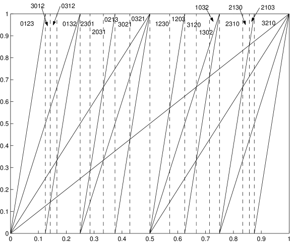
Figure 1: The $18$ allowed 4-patterns of the shift map $S_{2}:x\mapsto 2x(\mathop{\mathrm{m}od}1)$. For clarity, the allowed patterns have been written without angular parentheses nor separating commas. Note that the allowed patterns are ‘mirrored’ with respect to the central line, $x=1/2$.

Example 1

Figure 1 depicts the graphs of the identity (main diagonal), the shift (or sawtooth) map $S_{2}:x\mapsto 2x(\mathop{\mathrm{m}od}1)$, its second iterate, $S_{2}^{2}$, and its third iterate, $S_{2}^{3}$. The vertical, dashed lines rise at the endpoints of the intervals $P_{\pi}\neq\emptyset$ of points $x$ defining the allowed patterns $\pi\in\mathcal{S}_{4}$. We conclude that $S_{2}$ has $18$ allowed $4$-patterns and hence $6$ forbidden $4$-patterns, namely:

$$\left\langle 0,2,3,1\right\rangle,\left\langle 1,0,2,3\right\rangle,\left\langle 1,3,2,0\right\rangle,\left\langle 2,0,1,3\right\rangle,\left\langle 3,1,0,2\right\rangle,\left\langle 3,2,0,1\right\rangle.$$ (6)

We leave as an exercise to check that $S_{2}$ has no forbidden patterns of length $3$.

We turn next to the question of finding natural conditions on $f$ that allow the existence of forbidden patterns of any length. Given $\varepsilon>0$ arbitrarily small, there exists by Definition 2 a product partition $\iota_{0}$ such that

$$\left|h_{top}^{\ast}(f)-h_{top}^{\ast}(\mathbf{S}^{\iota})\right|<\frac{\varepsilon}{2}$$

whenever $\left\|\iota\right\|\leq\left\|\iota_{0}\right\|$. Furthermore, there exists by Definition 1 a length $L_{0}$ such that

$$\left|h_{top}^{\ast}(\mathbf{S}^{\iota})-\frac{1}{L}\log N(\mathbf{S}^{\iota},L)\right|<\frac{\varepsilon}{2}$$

whenever $L\geq L_{0}$, where $N(\mathbf{S}^{\iota},L)$ is the number of allowed ordinal $L$-patterns of the symbolic dynamic $\mathbf{S}^{\iota}$ with respect to the coarse-graining $\iota$. Therefore, chosen $\iota$ sufficiently fine and $L$ sufficiently large, we have

$$\left|h_{top}^{\ast}(f)-\frac{1}{L}\log N(\mathbf{S}^{\iota},L)\right|<\varepsilon,$$

hence,

$$N(\mathbf{S}^{\iota},L)=e^{Lh_{top}^{\ast}(f)}+\mathcal{O}_{L}(\varepsilon),$$ (7)

where the term $\mathcal{O}_{L}(\varepsilon)$ depends also on $L$, as indicated by the subindex, and $\mathcal{O}_{L}(\varepsilon)\rightarrow 0$ when $\varepsilon\rightarrow 0$ (or $\left\|\iota\right\|\rightarrow 0$). Since according to Stirling’s formula,

$$L!\varpropto\left(L/e\right)^{L}\sqrt{2\pi L}=e^{L(\log L-1)+(1/2)\log 2\pi L}$$

(where $\varpropto$ stands for “asymptotically”), the number of possible ordinal $L$-patterns, $\left|\mathcal{S}_{L}\right|=L!$, grows superexponentially with $L$, we conclude from (7) that the symbolic dynamic $\mathbf{S}^{\iota}$ has forbidden patterns whenever $h_{top}^{\ast}(f)$ is finite. Intuitively speaking, the same must happen with maps whose dynamic can be well approximated by simple observations.

Theorem 2

Let $I\subset\mathbb{R}^{q}$ be a finite interval and $f:I\rightarrow I$ a continuous map. Then

$$\lim_{\left\|\iota\right\|\rightarrow 0}N(\mathbf{S}^{\iota},L)=N(f,L),$$

where $N(f,L)$ is the number of allowed patterns of $f$ with length $L$.

[Proof.] Fix $L\geq 2$ and suppose that there exists an ordinal pattern $\pi(x)=\left\langle\pi_{0},...,\pi_{L-1}\right\rangle$ defined by $x\in I$ under $f$ that is not visible to any symbolic dynamic $\mathbf{S}^{\iota}$ with respect to a product partition $\iota$. Since ordinal patterns are defined by inequalities (see (5)), there exists by continuity $\eta>0$ such that $\left\|x-y\right\|<\eta$ implies $\pi(x)=\pi(y)$, the ordinal pattern defined by $y$. This means that, in the limiting process $\left\|\iota\right\|$ $\rightarrow 0$, we do take account of all ordinal $L$-patterns that the orbits of $f$ can produce.

From (7) it follows then,

Corollary 3

Under the hypotheses of Theorem 2, the number of allowed $L$-patterns of $f$ grows with $L$ as

$$\left|\{P_{\pi}\neq\varnothing:\pi\in\mathcal{S}_{L}\}\right|\varpropto e^{Lh_{top}^{\ast}(f)},$$ (8)

provided $h_{top}^{\ast}(f)<\infty$.

Since checking the technical condition $h_{top}^{\ast}(f)<\infty$ is in practice more difficult than checking directly the growth rate of the allowed patterns of $f$, we use now Theorem 1 to provide more natural conditions for (8).

Corollary 4

If $I\subset\mathbb{R}^{q}$ is a finite interval and $f:I\rightarrow I$ an expansive map with $h_{top}(f)<\infty$, then (8) holds true.

The bottom line is that interval maps have forbidden patterns under quite general conditions and that they proliferate superexponentially with the length $L$ as

$$\left|\{P_{\pi}=\varnothing:\pi\in\mathcal{S}_{L}\}\right|\varpropto L!-e^{Lh_{top}^{\ast}(f)}$$

(more on this in Sect. 4.2).

Apart from the superexponential scaling law with $L$, it is quite difficult to make more specific statements on the forbidden patterns of a given map $f$ like, for instance, the minimal length of its forbidden patterns. One important exception is the shift transformation on sequence spaces.

Example 2

As in (1), let $A^{\mathbb{N}_{0}}$ be the one-sided sequence space of the symbols $A=\{a_{1},a_{2},...,a_{\left|A\right|}\}$, where $a_{1}<a_{2}<...<a_{\left|A\right|}$, $A^{\mathbb{N}_{0}}$ being endowed with the lexicographic order $\preceq$ defined for $\mathbb{\alpha}\neq\mathbb{\alpha}^{\prime}$ as 

$$\mathbb{\alpha}\prec\mathbb{\alpha}^{\prime}\;\Leftrightarrow\left\{\begin{array}[]{cc}\;\mathbb{\alpha}_{i}=\mathbb{\alpha}_{i}^{\prime}&\mbox{for}\text{ }0\leq i\leq n\\ \text{\mbox{and}}&\\ \mathbb{\alpha}_{n+1}<\mathbb{\alpha}_{n+1}^{\prime}&\end{array}\right..$$ (9)

Furthermore, let $\Sigma:A^{\mathbb{N}_{0}}\rightarrow A^{\mathbb{N}_{0}}$ be the corresponding shift

$$(\mathbb{\alpha}_{0},\mathbb{\alpha}_{1},\mathbb{\alpha}_{2},...)\mapsto(\mathbb{\alpha}_{1},\mathbb{\alpha}_{2},\mathbb{\alpha}_{3},...).$$ (10)

Then one can prove [5]:

1. For every $L\leq\left|A\right|+1$, $\Sigma$ has no forbidden patterns.

2. For every $L\geq\left|A\right|+2$, $\Sigma$ has forbidden root patterns of length $L$. For instance if $\left|A\right|$ is even, then the ordinal patterns of length $L=\left|A\right|+2$

   $$\left\langle 0,2,...,\left|A\right|,\left|A\right|+1,...,3,1\right\rangle,$$

   $$\left\langle\left|A\right|+1,\left|A\right|-1,...,1,0,2,...,\left|A\right|-2,\left|A\right|\right\rangle$$

   and

   $$\left\langle\left|A\right|-1,\left|A\right|-3,...,1,0,2,...,\left|A\right|,\left|A\right|+1\right\rangle$$

   are forbidden. Moreover, if $\pi=\left\langle\pi_{0},\pi_{1},...,\pi_{L-2},\pi_{L-1}\right\rangle$ is forbidden for $\Sigma$, then its mirrored pattern

   $$\pi_{\text{\emph{mirrored}}}=\left\langle\pi_{L-1},\pi_{L-2},...,\pi_{1},\pi_{0}\right\rangle$$

   is also forbidden for $\Sigma$.

4 Properties of the forbidden patterns

To complete the picture, we briefly review in this section the three more important properties of forbidden patterns (see also [4, 5]).

4.1 Invariance under order-isomorphims

Since ordinal patterns are not directly related to measure-theoretical properties, isomorphic (or conjugate) dynamical systems need not have the same forbidden patterns, unless the isomorphism between them preserves not only measure but also linear order (supposing both state spaces are linearly ordered).

For instance, the graphical technique used in Figure 1 reveals that the logistic map $f(x)=4x(1-x)$, $0\leq x\leq 1$, has the forbidden $3$-pattern $\left\langle 2,1,0\right\rangle$ [4], i.e., there are no three consecutive points in any orbit generated by the logistic map, forming a strictly decreasing trio. However, it follows from the general results stated in Example 2 that the one-sided $(\frac{1}{2},\frac{1}{2})$-Bernoulli shift [7] has no forbidden patterns of length $3$, despite being conjugate to the logistic map (the interval $[0,1]$ endowed with the measure $\frac{dx}{\pi\sqrt{x(1-x)}}$). The reason is that the corresponding isomorphism, actually the symbolic dynamic $\mathbf{S}^{\iota}:[0,1]\rightarrow\{0,1\}^{\mathbb{N}_{0}}$ with respect to the generating partition $\iota=\{I_{0}=[0,\frac{1}{2}),I_{1}=[\frac{1}{2},1]\}$, is not order-preserving: e.g.,

$$\mathbf{S}^{\iota}(\tfrac{1}{4})=(0,\bar{1})<\mathbf{S}^{\iota}(\tfrac{3}{4})=(\bar{1}),$$

where the overbar denotes indefinite repetition of the binary digit and binary strings are ordered lexicographically, while

$$\mathbf{S}^{\iota}(\tfrac{1}{2})=(1,1,\bar{0})>\mathbf{S}^{\iota}(1)=(1,\bar{0}).$$

Definition 1

Given two linearly ordered sets $(X_{1},\leq_{1})$ and $(X_{2},\leq_{2})$, two maps $T_{1}:X_{1}\rightarrow X_{1}$ and $T_{2}:X_{2}\rightarrow X_{2}$ and an invertible map $\Phi:X_{1}\rightarrow X_{2}$ such that $\Phi\circ T_{1}=T_{2}\circ\Phi$, we say that $T_{1}$ and $T_{2}$ are order-isomorphic if $\Phi$ is order-preserving (i.e., $x\leq_{1}y$ implies $\Phi(x)\leq_{2}\Phi(y)$).

It is trivial that order-isomorphic maps have the same allowed (and, hence, forbidden) ordinal patterns. Let us see next an interesting example of an order-isomorphism.

Example 3

Let $A=\{0,1,...,b-1\}$ and consider the two-sided sequence space with alphabet $A$,

$$A^{\mathbb{Z}}=\{\mathbb{\alpha}=(\mathbb{\alpha}_{n})_{n\in\mathbb{Z}}=(...,\mathbb{\alpha}_{-1},\mathbb{\alpha}_{0},\mathbb{\alpha}_{1},...):\mathbb{\alpha}_{n}\in A\}.$$

With the notation $\mathbb{\alpha}_{-}$ for the ‘left sequence’ $(\mathbb{\alpha}_{-n})_{n\in\mathbb{N}}$ of the ‘bisequence’ $\mathbb{\alpha}\in A^{\mathbb{Z}}$ and $\mathbb{\alpha}_{+}$ for its ‘right sequence’ $(\mathbb{\alpha}_{n})_{n\in\mathbb{N}_{0}}$, we define a linear order $\preceq$ in $A^{\mathbb{Z}}$ by

$$\mathbb{\alpha}\prec\mathbb{\alpha}^{\prime}\;\Leftrightarrow\left\{\begin{array}[]{l}\;\mathbb{\alpha}_{+}<\mathbb{\alpha}_{+}^{\prime}\\ \text{\mbox{or}}\\ \mathbb{\alpha}_{-}<\mathbb{\alpha}_{-}^{\prime}\text{ \mbox{if} }\mathbb{\alpha}_{+}=\mathbb{\alpha}_{+}^{\prime}\end{array}\right.\text{ ,}$$ (11)

where $\leq$ between right (resp. left) sequences denotes lexicographical order in $A^{\mathbb{N}_{0}}$ (resp. $A^{\mathbb{N}}$), see (9). If $\mathcal{N}$ denotes the null set of bisequences $\mathbb{\alpha}$ eventually terminating in an infinite string of $(b-1)$s in either direction, then the map $\psi:A^{\mathbb{Z}}\backslash\mathcal{N}\rightarrow$ $[0,1)\times[0,1)\equiv[0,1)^{2}$ (here “ $\backslash$” stands for set difference) defined by

$$\psi:(\mathbb{\alpha}_{-},\mathbb{\alpha}_{+})\mapsto\left(\sum_{n=1}^{\infty}\mathbb{\alpha}_{-n}b^{-n},\sum_{n=0}^{\infty}\mathbb{\alpha}_{n}b^{-(n+1)}\right),$$ (12)

is one-to-one and order-preserving. As a matter of fact, the order (11) in $A^{\mathbb{Z}}$ corresponds via $\psi$ to the lexicographical order in $[0,1)^{2}$, so we may call $\preceq$ the lexicographical order in $A^{\mathbb{Z}}$. In sum, $\psi$ is an order-isomorphism, both $A^{\mathbb{Z}}\backslash\mathcal{N}$ and $[0,1)^{2}$ being endowed with the lexicographic order.

As way of application, consider the (non-continuous!) baker map, $B:[0,1)^{2}\rightarrow[0,1)^{2}$, where

$$B(x,y)=\left\{\begin{array}[]{lc}(2x,\frac{1}{2}y),&0\leq x<\frac{1}{2},\\ (2x-1,\frac{1}{2}y+\frac{1}{2}),&\frac{1}{2}\leq x<1.\end{array}\right.$$

If now $\overline{\Sigma}$ denotes a two-sided shift on two-symbol sequences, then $B$ and $\overline{\Sigma}$ are order-isomorphic, modulo the null set $\mathcal{N}$, via the ‘coding map’ $\psi:A^{\mathbb{Z}}\backslash\mathcal{N}\rightarrow$ $[0,1)^{2}$ given in (12). It follows that the baker map and the two-sided shift on two-symbol sequences have the same allowed and forbidden patterns.

Even more is true. First of all, one- and two-sided shifts on (bi-)sequences ordered lexicographically (see (9) and (11), respectively) can be proven to have the same forbidden patterns [5]. Furthermore, one can also prove along the same lines as in Example 3 that the sawtooth map $x\longmapsto 2x$ (mod 1) and the one-sided shift (10) on two-symbol sequences are order-isomorphic (modulo the null set of sequences terminating in $\bar{1}$). We conclude that the allowed and forbidden $4$-patterns of the baker map are precisely those exhibited in Figure 1 and listed in (6), respectively.

4.2 Growth with length: outgrowth patterns

According to Corollary 3, for every continuous self map $f$ on a finite $q$-dimensional interval with finite topological permutation entropy, there exists $\pi\in\mathcal{S}_{L}$, $L\geq 2$, which cannot occur in any orbit. Moreover, if $\pi=\left\langle\pi_{0},...,\pi_{L-1}\right\rangle$ is forbidden for $f$, then it is easy to see that the $2(L+1)$ patterns of length $L+1$,

$$\left\langle L,\pi_{0},...,\pi_{L-1}\right\rangle,\left\langle\pi_{0},L,\pi_{1},...,\pi_{L-1}\right\rangle,...,\left\langle\pi_{0},...,\pi_{L-1},L\right\rangle,$$

$$\left\langle 0,\pi_{0}+1,...,\pi_{L-1}+1\right\rangle,\left\langle\pi_{0}+1,0,\pi_{1}+1,...,\pi_{L-1}+1\right\rangle,...,\left\langle\pi_{0}+1,...,\pi_{L-1}+1,0\right\rangle,$$

are also forbidden for $f$. A weak form of the converse holds also true: if $\left\langle L,\pi_{0},...,\pi_{L-1}\right\rangle$, $\left\langle\pi_{0},L,...,\pi_{L-1}\right\rangle$, $...$, $\left\langle\pi_{0},...,\pi_{L_{0}-1},L\right\rangle\in\mathcal{S}_{L+1}$ are forbidden, then $\left\langle\pi_{0},...,\pi_{L-1}\right\rangle\in\mathcal{S}_{L}$ is also forbidden.

In turn, each of these forbidden patterns of length $L+1$ belonging to the ‘first generation’, will generate a ‘second generation’ of forbidden patterns of length $L+2$, not necessarily all different, etc.. Observe that all these forbidden patterns generated by $\pi$ in the $n$th generation have the form

$$\left\langle\ast,\pi_{0}+n,\ast,\pi_{1}+n,\ast,...,\ast,\pi_{L-1}+n,\ast\right\rangle\in\mathcal{S}_{N}$$ (13)

(the wildcard $\ast$ stands eventually for any other entries of the pattern), with $n=0,1,...,N-L$, where $N-L\geq 1$ is the number of wildcards $\ast\in\{0,1,...,n-1,L+n,...,N-1\}$ (with $\ast\in\{L,...,N-1\}$ if $n=0$ and $\ast\in\{0,...,N-L-1\}$ if $n=N-L$). Forbidden patterns of the form (13), where $\pi=\left\langle\pi_{0},...,\pi_{L-1}\right\rangle$ is forbidden, are called outgrowth forbidden patterns. If $\mathcal{S}_{N}^{out}(\pi)$ denotes the set of outgrowth forbidden $N$-patterns of $\pi$, the it can be proven [5] that there exist constants $0<c,d<1$ such that

$$(1-d^{N})N!<\left|\mathcal{S}_{N}^{out}(\pi)\right|<(1-c^{N})N!.$$ (14)

Forbidden patterns that are not outgrowth patterns of other forbidden patterns of shorter length are called forbidden root patterns since they can be viewed as the root of the tree of forbidden patterns spanned by the outgrowth patterns they generate, branching taking place when going from one length (or generation) to the next. Thus (14) shows that alone the number of outgrowth $N$-patterns of a given forbidden $L$-pattern, $N>L$, follows a superexponential growth law with $N$.

4.3 Robustness against noise

Finally, let us elaborate on the persistence of forbidden patterns when the observed data are distorted by small perturbations, a property we refer to as robustness against observational noise. As already mentioned in the Introduction, forbidden patterns are robust against observational noise on account of being defined by inequalities. Were not for this property, forbidden patterns would not be useful in applications.

The sort of applications we have in mind belong to the detection of determinism in univariate and multivariate time series analysis, since random real-valued time series have no forbidden patterns with probability $1$; see [4] for the intricacies of the scalar case when the sequences are finite and contaminated with (additive) white noise, i.e., when the time series have the form

$$z_{k}=f^{k}(x)+\eta_{k},$$ (15)

with $f$ being a one-dimensional interval map and $\eta_{k}$ real-valued (and properly bounded), independent, equally distributed (i.i.d.) random variables. A $2$-dimensional time series contaminated with white noise will be considered in the next section. The case of colored noise (i.e., random variables with correlation) is more difficult and is currently under investigation; ias a matter of fact, numerical sequences of the form (15) are often used to generate colored noise.

5 Numerical simulations

We demonstrate numerical evidence for the existence of forbidden ordinal patterns in multi-dimensional maps. Of course, direct simulation of dynamical systems directly yields only allowed order patterns. The failure to observe any given order pattern/permutation in any finite time series does not mean of course that it is forbidden (probability zero) but only that its probability is sufficiently low in the measure induced by the natural dynamics that it has not yet been seen.

However, with sufficiently reasonable $L$ (as effort and memory increases radically with $L$) and robust computational ability we can infer in many cases, robustness of forbidden patterns by examining the convergence of allowed patterns with $N$, the number of order patterns (of length $L$) emitted by the data generating source. In particular, we suggest examining the logarithmic ratio of the cardinality of all patterns to the number of observed patterns $\log\left(L!/P_{\text{obs}}\right)$ vs $\log N$. If a system has a “core” of forbidden patterns, as with deterministic systems, then we expect that this ratio will decline with $N$ and eventually level off with increasing $N$, assuming the asymptotic behavior can be observed. Here, $P_{\text{obs}}$ is the naive, biased-downward, estimator of the unknown $P_{\text{allowed}}$.

When $N$ is much larger than $P_{\text{allowed}}$, $P_{\text{obs}}$ is likely to be a good estimator, assuming most patterns have a reasonable probability of occurring. With increasing $L$, however, this is difficult to achieve practically because of memory limitations, as the identities and counts of each observed patterns (a subset of the allowed patterns) must be retained. The number of allowed patterns increases exponentially with $L$ in deterministic chaos, and faster than exponentially with noise, and therefore one must increase $N$, the number of iterates, substantially to permit a commensurately large number of distinct patterns to be actually observed.

This motivates using a superior statistical estimator of $P_{\text{allowed}}$. This equivalent problem has a significant history, motivated especially from the ecology community. Consider a situation where one can observe a finite sample of individual organisms, from a presumably large population. What is the estimated number of distinct species, the biodiversity, and how can we estimate this given the individual counts of observed species? (For reviews of approaches to this problem see [9, 10].) This is analogous to our situation where we can distinguish individual order patterns but each observation is drawn from the natural distribution induced by typical orbits of the dynamical system. For our needs we wish to go reasonably deep into the undersampled regime and impose few probabilistic priors. We adopt the non-parametric estimator of Chao [11], motivated by comments in the reviews and our experience, as a simple but reasonably effective improvement:

$$P_{\text{Chao}}=P_{\text{obs}}+\frac{c_{1}^{2}}{2c_{2}^{2}},$$ (16)

where $c_{k}$ are the “meta-counts” of observations, i.e. $c_{1}$ is the number of distinct ordinal patterns which were observed exactly once in the sample, $c_{2}$ the number which were observed exactly twice, etc. In practice this is accomplished by counting frequencies of observed patterns through a hash table, and in a second phase, counting the frequencies of such frequencies with a similar hash table. Note that if the sample size is particularly small (relative to what is necessary to see a substantial fraction of allowed patterns), $P_{\text{Chao}}$ will still be an underestimate. Consider that its maximum value is obtained with $c_{1}=N-1$ and $c_{2}=1$, i.e. one doubleton and all remaining observations being unique (all unique naturally leads to an undefined estimate), and so $P_{\text{Chao}}$ is bounded by $(P_{\text{obs}}^{2}+1)/2$. Bunge and Fitzpatrick [9] call $P_{\text{Chao}}$ to be an “estimated lower bound”. We believe that no statistical estimator can perform well in the extremely undersampled regime and there is no substitute for substantial computational effort when $L$ becomes sufficiently large; however, we will see an improvement over the naive estimator.

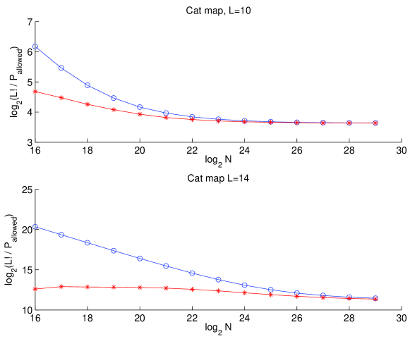
Figure 2: Convergence of estimated forbidden patterns with $N$, cat map. Blue circles (o) are for $P_{\text{allowed}}=P_{\text{obs}}$, red asterisks (*) have $P_{\text{allowed}}=P_{\text{Chao}}$. Top, $L=10$, bottom $L=14$. Both figures show clear evidence of convergence to a constant, evidence of true forbidden patterns as $N\rightarrow\infty$. In the lower figure especially, the improved estimator $P_{\text{Chao}}$ “senses” the approach to a convergence earlier than the naive counting estimator. Note the differing scales on the $y$-axes.

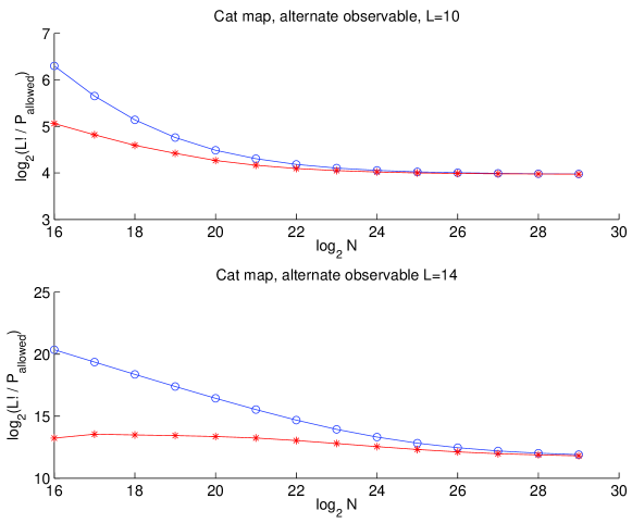
Figure 3: Convergence of estimated forbidden patterns with $N$, cat map, alternative observable. Blue circles (o) are for $P_{\text{allowed}}=P_{\text{obs}}$, red asterisks (*) have $P_{\text{allowed}}=P_{\text{Chao}}$. Top, $L=10$, bottom $L=14$. Both figures show clear evidence of convergence to a constant, evidence of true forbidden patterns as $N\rightarrow\infty$. In the lower figure especially, the improved estimator $P_{\text{Chao}}$ “senses” the approach to a convergence earlier than the naive counting estimator. Note the differing scales on the $y$-axes.

Our first numerical example is Arnold’s “cat” map: $(x,y)\rightarrow(x+y\mod 1,x+2y\mod 1)$. We start with initial conditions drawn uniformly in $[0,1)\times[0,1)$, and iterate. Ordinal patterns are computed using order relations on the $x$-coordinate only. Figure 2 shows the strong numerical evidence for forbidden patterns characteristic of deterministic systems. As a demonstration of the genericity of the results, Figure 3 shows the equivalent except that the observable upon which order patterns were computed is $3x^{3}-y$. Results are nearly identical, as one expects.

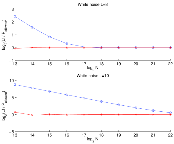
Figure 4: Convergence of estimated forbidden patterns with $N$, i.i.d. noise. Blue circles (o) are for $P_{\text{allowed}}=P_{\text{obs}}$, red asterisks (*) have $P_{\text{allowed}}=P_{\text{Chao}}$. Top, $L=8$, bottom $L=10$. $P_{\text{obs}}$ shows convergence to zero forbidden pattterns; $P_{\text{Chao}}$ estimates zero forbidden patterns well before convergence of naive estimator.

By comparison, consider Figure 4, generated by an i.i.d. noise source (ordinal patterns are insensitive to changes in distribution). Here, the observed patterns imply convergence to zero forbidden patterns with increasing $N$. More remarkably the estimator $P_{\text{Chao}}$ senses this long before and predicts zero forbidden patterns with orders of magnitude lower $N$, apparently because the assumptions made by the estimator of equiprobable patterns for both observed and unobserved are exactly fulfilled.

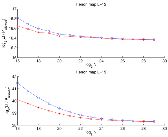
Figure 5: Convergence of estimated forbidden patterns with $N$, Hénon map. Blue circles (o) are for $P_{\text{allowed}}=P_{\text{obs}}$, red asterisks (*) have $P_{\text{allowed}}=P_{\text{Chao}}$. Top, $L=12$, bottom $L=19$. Both naive and improved estimators show convergence to a finite number of forbidden patterns with increasing $N$. Note scale of $y$-axes.

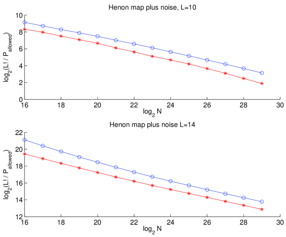
Figure 6: Lack of cnvergence of estimated forbidden patterns with $N$, Hénon map with additive i.i.d. noise. Blue circles (o) are for $P_{\text{allowed}}=P_{\text{obs}}$, red asterisks (*) have $P_{\text{allowed}}=P_{\text{Chao}}$. Top, $L=12$, bottom $L=19$. Both naive and improved estimators show continued increase in allowed patterns (decrease in forbidden patterns) with increasing $N$.

The cat map may be seen as too “easy” and so we turn to a chaotic system, the Hénon map, $(x,y)\rightarrow(1-ax^{2},bx),\,a=1.4,b=0.3$, observable being the $x$-coordinate. This map is not uniformly hyperbolic, more characteristic of real dynamics seen in nature. In Figure 5, we see convergence to a finite core of forbidden patterns with larger $N$. Note that the performance of $P_{\text{Chao}}$ is still improved over the naive estimator but it is not as good as with noise, because with real dynamics there is a wide variation in the probability of the various allowed patterns, and so larger $N$ feels the ’tail’ of the distribution of rare patterns. By comparison consider Figure 6, which shows results from the same dynamics but each observable was contaminated with uniform i.i.d noise $\eta\in[0,0.2)$. This time, increasing $N$ clearly shows increasing allowed/decreasing forbidden patterns, proportional to $N$ as expected with noise. The behavior with $N$ cleanly distinguishes low-dimensional dynamics from noise.

As a philosophical point it is true that the “noise” generator in a computer software is but a deterministic dynamical system on its own, but in practice it has an extremely long period and virtually no correlation, and hence if one wanted to see order pattern scaling different from true noise, one would need exceptionally long $L$ and impractically astronomical memory requirements. We use a validated high-quality random number generator [12] from the Boost C++ library.

6 Conclusion

We showed that $n$-dimensional interval maps have forbidden ordinal patterns under the following two sufficient conditions: (i) continuity, and (ii) finite topological permutation entropy (Corollary 3). The second condition, that can be difficult to check, may be replaced by (ii’) finite topological entropy if the first condition is replaced by (i’) expansiveness (Corollary 4). In any case, we conjecture as a working hypothesis that the existence of forbidden patterns is a general feature of the interval maps encountered in practice.

Interestingly enough, the existence of forbidden patterns can be used as an indicator of determinism in univariate and multivariate time series analysis, since sequences generated by unconstrained random processes taking values on intervals have no forbidden patterns with probability one. The application of these ideas requires some care since real sequences are finite (making possible that random sequences have ‘false’ forbidden patterns with finite probability) and noisy (blurring the difference between determinism and randomness). The numerical simulations of Sect. 5 have provided ample evidence of all these issues, in particular of the robustness of forbidden patterns against observational white noise. In so doing we have also used Chao’s estimator for the number of classes in a population.

References

- [1] J.M. Amigó, M.B. Kennel and L. Kocarev, The permutation entropy rate equals the metric entropy rate for ergodic information sources and ergodic dynamical systems, Physica D 210 (2005) 77-95.
- [2] J.M. Amigó and M.B. Kennel, Topological permutation entropy, Physica D 231 (2007) 137-142.
- [3] J.M. Amigó, L. Kocarev and J. Szczepanski, Order patterns and chaos, Phys. Lett. A 355 (2006), 27-31.
- [4] J.M. Amigó, S. Zambrano and M.A.F. Sanjuán, True and false forbidden patterns in deterministic and random dynamics, Europhys. Lett. 79 (2007) 50001-p1, -p5.
- [5] J.M. Amigó, S. Elizalde and M.B. Kennel, Forbidden patterns and shift systems, J. Combin. Theory, Series A (to appear). Available in www.arxiv.org, preprint arXiv:0707.4628v2.
- [6] C. Bandt, G. Keller and B. Pompe, Entropy of interval maps via permutations, Nonlinearity 15 (2002) 1595-1602.
- [7] A. Katok and B. Hasselblatt, Introduction to the Modern Theory of Dynamical Systems, Cambridge University Press, Cambridge, 1998.
- [8] P. Walters, An Introduction to Ergodic Theory (Springer Verlag, New York, 1982).
- [9] J. Bunge and M. Fitzpatrick, Estimating the Number of Species: A Review, Jour. Amer. Stat. Assoc., 88 (1993) 364-373.
- [10] J. Hughes, J. Hellman, T.H. Rickets and B.J.M. Bohannan, Counting the Uncountable: Statistical Approaches to Estimating Microbial Diversity, Applied and Environ. Microbiology 67 (2001) 4399-4406.
- [11] A. Chao, Nonparametric Estimation of the Number of Classes in a Population, Scandinavian Journal of Statistics, Theory and Applications, 9 (1984) 265-270.
- [12] M. Matsumoto and T. Nishimura, Mersenne Twister: A 623-dimensionally equidistributed uniform pseudo-random number generator, ACM Trans. on Modeling and Computer Simulation, 8 (1998) 3-30.