A Markov process associated with plot-size distribution in Czech Land Registry and its number-theoretic properties

Abstract

The size distribution of land plots is a result of land allocation processes in the past. In the absence of regulation this is a Markov process leading an equilibrium described by a probabilistic equation used commonly in the insurance and financial mathematics. We support this claim by analyzing the distribution of two plot types, garden and build-up areas, in the Czech Land Registry pointing out the coincidence with the distribution of prime number factors described by Dickman function in the first case.

The distribution of commodities is an important research topic in economy – see [CC07] for an extensive literature overview. In this letter we focus on a particular case, the allocation of land representing a non-consumable commodity, and a way in which the distribution is reached. Generally speaking, it results from a process of random commodity exchanges between agents in the situation when the aggregate commodity volume is conserved, in other words, one deals with pure trading which leads to commodity redistribution.

Models of this type were recently intensively discussed [SGG06] and are usually referred to as kinetic exchange models. Our approach here will be different, being based on the concept known as perpetuity. The latter is a random variable $D$ that satisfies a stochastic fixed-point equation the form

$$D\triangleq a(D+1)\,,$$ (1)

where $a$ and $D$ are independent random variables and the symbol $\triangleq$ means that the two sides of the equation have the same probability distribution; by an appropriate scaling, of course, the value one in (1) can be replaced by any fixed positive number. It is supposed that the distribution $P(a)$ of the variable $a$ is given and one looks for the distribution $Q(D)$ of $D$.

The equation (1) has a solution provided the variable $a$ satisfies $\mathrm{mean}(\log a)<0$, cf. [Ve79]. It appears in the literature under various names depending on the field of application; it is known as the Vervaat perpetuity [Ve79], stochastic affine mapping, random difference equation, stochastic fix point equation, and so on. Before proceeding further, let us remark that the equation (1) looks innocent but it is not. The situation when $a$ is a Bernoulli variable is tricky, in particular, it was proved in [BR01] that the probability measure associated with $Q(D)$ is singularly continuous in this case.

Perpetuities themselves appear in different contexts. In the insurance and financial mathematics, for instance, a perpetuity represents the value of a commitment to make regular payments [GM00]. Another situation where we meet perpetuities arises in connection with recursive algorithms such as the selection procedure Quickselect – see, e.g., [HT02] or [MMS95], and they also describe random partitioning problems [Hu05].

Related quantities emerge, however, even in purely number-theoretic problems, in particular, in the probabilistic number theory they describe the largest factor in the prime decomposition of a random integer — see, for instance, [DG93, Cor. 2] or [HT93, MV07] and references therein. Specifically, the following claim is valid:
Proposition: Denote by $p(D,X)$ the probability that a random integer $n\in(1,X)$ has its greatest prime factor $\leq X^{1/D}$. The limit $Q(D)=\lim_{X\to\infty}p(D,X)$ exists and coincides with the solution of the equation $D\triangleq a(D+1)$ corresponding to the uniform distribution, $P(a)=1$.
Recall that the respective $Q(D)$ is known in the number theory as the Dickman function [BS07].

Let us pass now to our main subject which is the land plot distribution. We observe that the present sizes of the plots result from repeated land redistribution — land purchases and sales — in the past which represents a complex allocation process.

In attempt to understand it within a simple model, consider first a situation where the overall area is fixed and there are only three land owners; one can think about a small island having just three inhabitants. We consider a discrete time and denote by $D_{j}(n),\,j=1,2,3,$ the area of the land owned by the respective holder at time $t=n$ assuming that the overall area is equal to one. Consequently, the triple $\{D_{k}(n):\>k=1,2,3\}$ belongs for all $n=1,2,..$ to a 3-simplex, $D_{1}(n)+D_{2}(n)+D_{3}(n)=1$. The land trading on the island proceeds as follows: two holders $j,k$ with $j,k\in\{1,2,3\}$ such that $j\neq k$ are picked randomly and they trade their lots according to the rule

$$D_{j}(n+1) = a_{n}[D_{j}(n)+D_{k}(n)]$$

$$D_{k}(n+1) = (1-a_{n})[D_{j}(n)+D_{k}(n)]$$ (2)

where $a_{n}\in(0,1)$ are independent equally distributed random numbers. (We suppose that no land exchange involves all the three holders simultaneously.) Let us take for simplicity $j=1$ and $k=2$. The simplex condition gives $D_{1}(n)+D_{2}(n)=1-D_{3}(n)$, thus the relation (A Markov process associated with plot-size distribution in Czech Land Registry and its number-theoretic properties) implies $D_{1}(n+1)=a_{n}(1-D_{3}(n)$. In a steady situation the areas $D_{k}$ posses identical distributions equal to the distribution of the same random variable $D$; the replacement of $D_{1}$ and $D_{3}$ by independent copies of $D$ then leads to the equation $D\triangleq a(1-D)$. A simple substitution $D\rightarrow-D$ and $a\rightarrow-a$ leads finally to the equation (1), however, the distribution of $D$ is, of course, invariant under such a transformation, up to a mirror image. Consequently, the land trading on our island with three inhabitants leads formally to the lot area distribution described by the perpetuity equation (1). Notice that the constant $1$ appearing in it comes from the simplex constraint $D_{1}+D_{2}+D_{3}=1$; it can be regarded as a manifestation of the fact that the overall area is preserved in the trading.

There is another argument that leads to the same equation and which can be applied to the case of numerous land traders. The plot size $D(n)$ owned at the instant $n$ by a chosen one of them can be regarded as a result of two independent actions. The first step is the sale of a random fraction $a_{n}$ of the property owned at time $n\!-\!1$, i.e. $\>D_{n-1}\rightarrow a_{n}D_{n-1}$. The following step is the purchase of a new piece of land of a size $d_{n}$ and adding it to the one mentioned. In combination, these actions give

$$D_{n}=a_{n}D_{n-1}+d_{n}\,,\quad n=1,2,\dots\,.$$ (3)

The process is obviously of Markov type and the distribution of the plot sizes to which it converges is given by the equation $D\triangleq aD+d$ where $d$ is the random variable associated with the acquisitions. In fact, convergence of the process is closely related to the existence of solution to this equation [Ve79]. The process is linked to the Dickman function in case that the two random variables coincide, $d_{n}=a_{n}$ for all $n\in\mathbb{Z}_{+}$, and they are identically distributed; then (3) obviously leads to (1). From the point of land plot reallocations such an assumption is an idealization and it is formally exact – as mentioned above – for three traders only. It is an open question to what extent this distribution changes in situations with a larger number of players involved.

To understand better that how the Dickmann function can arise in the process, we observe that the solution of (1) is obtained formally as the following infinite sum [Ve79],

$$D=\sum_{n=1}^{\infty}\prod_{k=1}^{n}a_{1}a_{2}...a_{k}\,,$$ (4)

where $a_{1},a_{2},...,a_{k},...$ are independent uniformly distributed random variables. On the other hand, the Markov process (3) leads in our particular case, $d_{k}=a_{k}$, to

$$D_{n+1}=a_{n}+a_{n}a_{n-1}+a_{n}a_{n-1}a_{n-2}+..+a_{n}a_{n-1}a_{n-2}...a_{1}D_{1}\,,$$ (5)

where $D_{1}$ is the initial holding of the trader which we put equal to one. We may naturally relabel the variables and to write the right-hand side of (5) also as $a_{1}+a_{1}a_{2}+\cdots$; it is crucial that this leads to the same random variable $D_{n+1}$ since all the $a_{k}$’s are independent and equally distributed. In this form the relation between (4) and (5) is clearly seen; the question is whether the two quantities are close to each other in the situation we are interested in. The point is that the number of the trading steps is of course finite and not very large. Even without big historical disturbances we can hardly expect the free land trading to have a history longer than roughly three centuries. Assuming that a given plot is traded once in a generation we can thus run the process (5) realistically up to $n\lesssim 10$.

Luckily enough for us the convergence of (5) to (4) is rather fast: using the mentioned relabelling we find

$$D-D_{n+1}=a_{1}a_{2}a_{3}...a_{n}\widetilde{D}\,,$$ (6)

where $D$ and $\widetilde{D}$ are statistically equivalent. Denoting as usual by $\mathbb{E}(a)$ the mean of $a$, we get therefore

$$\mathbb{E}(D-D_{n+1})=\mathbb{E}(a)^{n}\mathbb{E}(\widetilde{D})=2^{-n}\,,$$ (7)

since $a$ is identically distributed in $(0,1)$ by assumption and $\mathbb{E}(\widetilde{D})=1$, which means that the convergence is exponentially fast. But this is not all, one can also show that the convergence is extremely shape robust. Indeed, take the Markov rule $D_{n+1}=a_{n}(D_{n}+1)$ and denote by $G_{n}(t)$ the probability that $D_{n}<t$. For the uniformly distributed variable $a$ we then have

$$G_{n+1}(t)=\int_{0}^{1}G_{n}\left(\frac{t}{a}-1\right)\mathrm{d}a\,,$$ (8)

and consequently, the densities $g_{n}(t):=G_{n}^{\prime}(t)$ satisfy

$$g_{n+1}(t)=\int_{0}^{1}g_{n}\left(\frac{t}{a}-1\right)\frac{\mathrm{d}a}{a}\,;$$ (9)

the support of all these functions lies by definition of the nonnegative real axis, $G_{n}(t)=g_{n}(t)=0$ for $t<0$. A simple substitution $u=t/a-1$ then gives finally a relation between the densities $g_{n+1}$ and $g_{n}$, namely

$$g_{n+1}(t)=\int_{t-1}^{\infty}g_{n}(u)\frac{\mathrm{d}u}{u+1}\,.$$ (10)

Let us now start with the situation far from the expected equilibrium assuming, for instance, that all the owners have at the initial instant land plots of the same are, i.e. $g_{1}(t)=\delta(t-1)$; then (10) gives

$$g_{2}(t)=\left\{\begin{array}[]{lcl}\frac{1}{2}&\quad\mathrm{if}\;\;t\in[0,2)\\[2.0pt] 0&\quad\mathrm{if}\;\;t>2\end{array}\right.\qquad g_{3}(t)=\left\{\begin{array}[]{lcl}\frac{1}{2}\ln 3&\quad\mathrm{if}\;\;t\in[0,1]\\[2.0pt] \frac{1}{2}\ln\left(\frac{3}{t}\right)&\quad\mathrm{if}\;\;t\in[1,3]\\[2.0pt] 0&\quad\mathrm{if}\;\;t>3\end{array}\right.$$

and so on. It can be seen easily from (10) that the functions $g_{n}(t),n=3,4,\cdots$, have the following properties: $g_{n}(t)=c_{n}$ for $t\in(0,1)$ where $c_{n}$ is a constant depending on $n$ only, and moreover, $g_{n}(t)$ is decreasing for $t\in[1,n]$ and $g_{n}(t)=0$ holds for $t>n$. Furthermore, we have $c_{n}\to\mathrm{e}^{-\gamma}$ as $n\to\infty$ with $\gamma$ being the Euler–Mascheroni constant — note that $\mathrm{e}^{-\gamma}$ is the value of the Dickman function for $t\in(0,1)$. Hence even if the original distribution had nothing in common with the Dickman function, the densities $g_{n}(t)$ are form robust and approach rapidly such a shape. In fact integrating further we find that the densities $g_{n}$ for $n>3$ are already very close to the Dickman limit $g_{\infty}$.

The conclusion for our model is that there is a chance to see the equilibrium situation in the land plot distributions provided the trading go undisturbed for at least four generations. If this is the case it makes sense to ask about a relation between the plot distribution and the equation (1); it is clear that only an inspection of actual data can show whether such a model assumption is good or not.

Let us thus look whether these considerations have something in common with land plot distribution in reality. One has to be cautious, of course, when choosing which types of plots are to be considered. Recall, for instance, that A. Abul-Magd tried recently to describe the wealth distribution in the ancient Egyptian society using areas of the house found by the excavations in Tell el-Amarna [AM02]. Their distribution exhibited a Pareto like distribution [Pa1897] known to describe the wealth allocation among individuals. It has an algebraic tail, and therefore it behaves in a way different from the Vervaat perpetuity for constant $P(a)$; recall that the Dickman function $Q(D)$, for instance, satisfies asymptotically the inequality $Q(D)<D^{-D}$ for large $D$. It is not surprising, however, that this case does not fit into our scheme, the aggregate volume being not locally conserved: upgrading a house as a result of one’s wealth need not affect the areas of the neighbouring houses.

The land plots we look for have to satisfy several criteria. As the above example suggests, they have to be arranged in connected areas, so that the gain of a purchaser is the same as the loss of the corresponding seller. At the same time, they must be divisible so one can sell and buy parts of them. Choosing such a plot type, one can look into the land registry where the present holdings are recorded. As we have said they are the result of repeated land purchase and land sell done by the ancestors in the past, but we are not going to look into the history being interested in the resulting distribution. We have to make sure, however, that the process was not affected by the outside influences like agrarian reforms or other forms of redistribution en gros.

One plot type suitable for our purpose are gardens in urban areas. We used the Czech real estate cadastre concentrating on the sizes of four thousand gardens in the urban area of the towns Rychnov nad Kněžnou and Dobruška in East Bohemia. To compare their distribution with the perpetuity result mentioned above we need, of course, a proper normalization: we choose the scale in which the mean size of the plot is equal to one. The result confirms our conjecture: the probability distribution of the garden areas coincides with the Dickman function as shown in Figure 1.

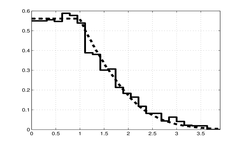
Figure 1: The probability density of the normalized garden areas (full line) is compared with the Dickman function (dashed line). We have used areas of 4000 gardens located in the two towns.

This finding can be easily understood. Gardens in urban areas are desirable properties, and as a result, any piece of a garden is equally good for the market. This means the process (A Markov process associated with plot-size distribution in Czech Land Registry and its number-theoretic properties) goes on with the variables $a$ and $d$ approximately homogeneously distributed over the interval $(0,1)$, so that the Dickman function gives a good fit confirming our expectation. Another conclusion we can make without looking into a detailed history is that the overall area of gardens in these towns did not change significantly in the course of the time.

Another suitable land plot type recorded in the cadaster which was not affected by agrarian reforms are yards and the build-up areas. In the latter case we take into account the areas only without paying attention to the type (number of floors, etc.) of the buildings which may be constructed on them. The situation is somewhat different from the garden distribution case, since now we need not restrict ourselves to the urban areas. This enables us to work with a much larger data set; altogether we employed data about 47000 yards and build-up areas.

The allocation process is different because it is not conservative in this case. In the course of time a new size of build-up area or yard can be a result of merging a number of smaller areas into a larger one, and at the same time, a larger area can come from the transformation of another land type into the building land. To describe such a process we use again the equation (1) with the uniformly distributed variable $a$ supposing that all changes occur with equal probability, however, we change the variable range taking $a\in(0,A)$ with $A>1$ to take into account the fact that the build-up area can expand. The result is plotted on the figure 2 and we see that choosing $A=1.52$ we get an excellent fit.

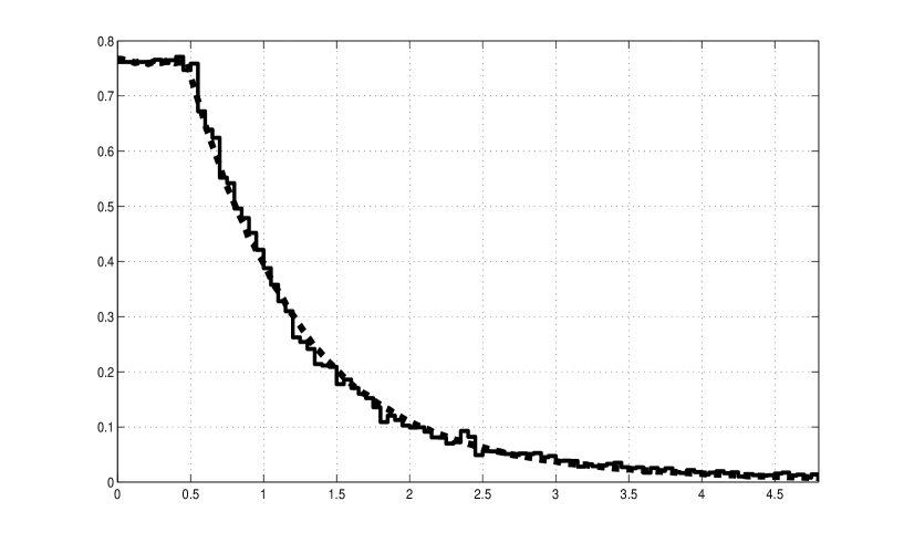
Figure 2: The probability density of the normalized sizes of the yard and build-up areas (full line) compared with the solution of eq. (1) with uniformly distributed $a\in(0,1.52)$ (dashed line). We have used the sizes of 47000 yards and build-up areas.

It would be interesting to test the concept described here on other plot types such as the distribution of fields or forests. For this purpose, unfortunately, the Czech land registry is not suitable because in this case the distribution was formed not only by standard market forces but also by processes like collectivization, etc. A brief look at the corresponding data shows that the distributions cannot be described with the help of (1) with a symmetric distribution $P(a)$.

Acknowledgement: We thank the referees for useful remarks. The research was supported by the Czech Ministry of Education, Youth and Sports within the project LC06002. The cooperation of the Land Registry District Office in Rychnov nad Kněžnou is gratefully acknowledged.

References

- [AM02] A.Y. Abul-Magd: Wealth distribution in an ancient Egyptian society, Phys. Rev. E66 (2002), 057104 .
- [BR01] M. Baron, A.L. Rukhin: Perpetuities and asymptotic change-point analysis, Stat. and Probab. Lett. 55 (2001), 29–38.
- [BS07] W.D. Banks, I.E. Shparlinski: Integers with a large smooth divisors, Integers 7 (2007), A17; see also arXiv:math.NT/0601460
- [CC07] A. Chatterjee, B.K. Chakrabarti: Kinetic exchange models for income and wealth distributions, arXiv:0709.1543 [physics.soc-ph]
- [DG93] P. Donnelly, G. Grimmett: On the asymptotic distribution of large prime factors, J. Lond. Math. Soc. 47 (1993), 395–404.
- [Du90] D. Dufresne: The distribution of a perpetuity with application to risk theory and pension funding, Scand. Actuarial J. (1990), 750–783.
- [GM00] Ch.M. Goldie, R.A. Maller: Stability of perpetuities, Ann. Probab. 28 (2000), 1195–1218.
- [HT93] A. Hildebrand, G. Tenebaum: Integers without large prime factors, J. de Théorie des Nombres de Bordeaux 5 (1993), 411–484.
- [Hu05] T. Huillet: Random partitioning problems involving Poisson point processes o the interval, Int. J. Pure Appl. Math. 24 (2005), 143–179.
- [HT02] H.–K. Hwang, T.–H. Tsai: Quickselect and the Dickman function, Combin. Probab. Comput. 11 (2002), 353–371.
- [MMS95] H. Mahmoud, R. Modarres, R. Smythe: Analysis of QUICKSELECT: an algorithm for order statistics, RAIRO Inform. Theor. Appl. 29 (1995), 255- 276.
- [Pa1897] V. Pareto: Course d’Economie Politique, Macmillan, Paris 1897.
- [SGG06] E. Scalas, M. Gallegati, E. Guerci, D. Mas, A. Tedeschi: Growth and allocation of resources in economics: The agent-based approach, Physica A370 (2006), 86–90.
- [Ve79] W. Vervaat: On a stochastic difference equation and a representation of of non-negative infinitely divisible random variables, Adv. Appl. Prob. 11 (1979), 750–783.
- [MV07] E.W. Weisstein: Dickman Function, from MathWorld – A Wolfram Web Resource, http://mathworld.wolfram.com/DickmanFunction.html.