Atom Fock state preparation by trap reduction

Abstract

We study the production of low atom number Fock states by reducing suddenly the potential trap in a 1D strongly interacting (Tonks-Girardeau) gas. The fidelity of the Fock state preparation is characterized by the average and variance of the number of trapped atoms. Two different methods are considered: making the trap shallower (atom culling [A. M. Dudarev et al., Phys. Rev. Lett. 98, 063001 (2007)], also termed “trap weakening” here) and making the trap narrower (trap squeezing). When used independently, the efficiency of both procedures is limited as a result of the truncation of the final state in momentum or position space with respect to the ideal atom number state. However, their combination provides a robust and efficient strategy to create ideal Fock states.

The generation of Fock states with a definite, controlled atomic number is a highly desirable objective both from fundamental and applied points of view. They may be useful for studying few particle interacting systems Phillips ; tunn , entanglement e , or number and spin-squeezed atomic systems r1 ; r2 . Production of fotonic Fock states r3 and interferometric schemes for sub-shot-noise sensitivity approaching the Heisenberg limit Heislimit do also require input Fock states.

A necessary step towards this goal is the development of atom counting devices paving the way into quantum atom statistics atomcounting . Indeed a technique with nearly unit efficiency has already been demonstrated CSMHPR05 . Moreover, the recently proposed method of atom culling by making the atom trap shallower (in the following also termed “trap weakening”) CSMHPR05 ; DRN07 has achieved sub-Poissonian atom-number fluctuations for $60-300$ trapped atoms when adiabatic conditions were fulfilled, i.e., when the trap depth is varied slowly. (The reference case of Poissonian statistics is realized by the number of particles in a small volume of a classical ideal gas.) In this method the initial state is assumed to be a ground state for an unknown number of bosons, in general smaller than the maximum capacity of the initial trap (this is, the maximum number of particles that can be confined in the trap). This capacity depends on the trap characteristics and interatomic interaction. As the barrier height of the trap is slowly reduced and the maximum capacity is surpassed, the excess of atoms will leave the trap to produce eventually the Fock state corresponding to the maximum capacity of the final trap configuration. For a pictorial representation see Fig. 1 (upper panel).

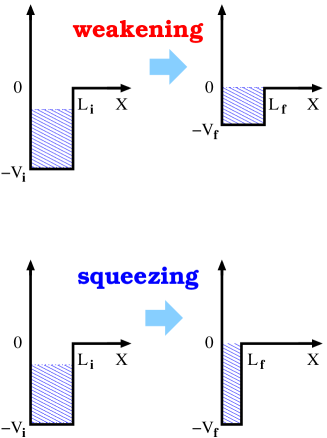
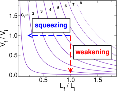
Figure 1: (color online) Schematic potential change for trap weakening and squeezing, where $L_{i}$ and $L_{f}$ are the initial and final well widths, and $V_{i}$ and $V_{f}$ the initial and final trap depths, respectively. Each solid line in the contour plot represents an isospectral family of traps at the threshold of a new bound state (for the initial trap $2mV_{i}L_{i}^{2}/\hbar^{2}=25\pi^{2}$, $C_{f}$ being the final trap capacity). A transition between two given families is achieved reducing the trap capacity. The bound energy levels are pushed up and the higher ones cross the continuum threshold so that the excess of atoms escapes from the trap.

A theoretical analysis has shown the basic properties of atom culling regarding the final average number as a function of the trap well depth and atom-atom interaction strength, covering the limits of the Tonks-Girardeau (TG) gas and the mean-field regime DRN07 : a weaker dependence on laser fluctuations of the height of the barrier that forms the trap will be favoured by strong interatomic interactions that separate the energy levels. This motivates the present work, in which we focus on the strongly interacting 1D TG limit, optimal for atom culling, and examine the average number and fluctuations of the trapped atoms. Particular attention is paid to the sudden regime, corresponding to the “worst case scenario” of an abrupt change from the initial to the final trap. We show that, even in this case, a state arbitrarily close to the ideal Fock state may be robustly produced by combining weakening and squeezing of the trap, the two basic processes represented schematically in Fig. 1.

I Atom statistics

Ultracold bosonic atoms in waveguides tight enough so that the transverse degrees of freedom are frozen out, are well described by the Lieb-Liniger (LL) model LieLin63 . In the strongly interacting limit Olshanii98 ; PSW00 (for low densities and/or large one-dimensional scattering length) a LL gas tends to the TG gas, which plays a distinguished role in atom statistics since its spatial antibunching has been predicted Kheruntsyan03 , and observed exp . The system exhibits “fermionization” Girardeau60 , i.e., the TG gas and its “dual” system of spin-polarized ideal fermions behave similarly, and share the same one-particle spatial density as well as any other local-correlation function, while differ on the non-local correlations.

The fermionic many-body ground state wavefunction of the dual system is built at time $t=0$ as a Slater determinant for $N_{i}$ particles, $\psi_{F}(x_{1},\dots,x_{N_{i}})=\frac{1}{\sqrt{N_{i}!}}{\rm det}_{n,k=1}^{N_{i}}\varphi_{n}^{i}(x_{k})$, where $\varphi_{n}^{i}(x)$ is the $n-$th eigenstate of the initial trap, whose time evolution will be denoted by $\varphi_{n}(x,t)$ whenever the external trap is modified. The bosonic wave function, symmetric under permutation of particles, is obtained from $\psi_{F}$ by the Fermi-Bose (FB) mapping Girardeau60 ; CS99 $\psi(x_{1},\dots,x_{N_{i}})=\mathcal{A}(x_{1},\dots,x_{N_{i}})\psi_{F}(x_{1},\dots,x_{N_{i}})$, where $\mathcal{A}=\prod_{1\leq j<k\leq N_{i}}{\rm sgn}(x_{k}-x_{j})$ is the “antisymmetric unit function”. Since $\mathcal{A}$ does not include time explicitly, it is also valid when the trap Hamiltonian is altered, and the time-dependent density profile resulting from this change can be calculated as GW00b $\rho(x,t)=N_{i}\!\!\int|\psi(x,x_{2},\dots,x_{N_{i}};t)|^{2}{\rm d}x_{2}\cdots{\rm d}x_{N_{i}}=\sum_{n=1}^{N_{i}}|\varphi_{n}(x,t)|^{2}.$ By reducing the trap capacity some of the $N_{i}$ atoms initially confined may escape and $N$ will remain trapped. To determine whether or not sub-Poissonian statistics or a Fock state are achieved in the reduced trap we need to calculate the atom-number fluctuations. We proceed by characterizing the TG trapped state by means of its variance $\sigma_{N}^{2}=\langle N^{2}(t)\rangle-\langle N(t)\rangle^{2}$. First note the general relation

$$\langle\widehat{n}(x)\widehat{n}(x^{\prime})\rangle_{t}\!\! = \!\!\langle:\widehat{n}(x)\widehat{n}(x^{\prime}):\rangle_{t}+\delta(x-x^{\prime})\langle\widehat{n}(x)\rangle_{t},$$ (1)

where the number field operator is $\widehat{n}(x)=\Psi^{\dagger}(x)\Psi(x)$, $\Psi(x)$, $\Psi^{\dagger}(x)$ are the annihilation and creation operators at point $x$, and $:\quad:$ denotes normal ordering. In particular, within the Tonks-Girardeau regime,

$$\langle\widehat{n}(x)\widehat{n}(x^{\prime})\rangle_{t} = D(x,x^{\prime};t)+\delta(x-x^{\prime})\rho(x,t),$$ (2)

with GWT01

$$D(x,x^{\prime};t) = \!\!N_{i}(N_{i}-1)\!\!\int\!\prod_{i=3}^{N_{i}}{\rm d}x_{i}|\psi(x,x^{\prime},x_{3},\cdots,x_{N_{i}};t)|^{2}$$ (3)

$$= \rho(x,t)\rho(x^{\prime},t)-|\Delta_{N_{i}}(x,x^{\prime},t)|^{2},$$

and

$$\Delta_{N_{i}}(x,x^{\prime};t)=\sum_{n=1}^{N_{i}}\varphi_{n}(x,t)^{*}\varphi_{n}(x^{\prime},t).$$ (4)

The mean value of the number of particles within the trap and of its square can be obtained by integrating over $x,x^{\prime}$,

$$\langle N(t)\rangle = \int_{0}^{L_{+}}{\rm d}x\rho(x,t),$$

$$\langle N^{2}(t)\rangle = \int_{0}^{L_{+}}\int_{0}^{L_{+}}{\rm d}x{\rm d}x^{\prime}\langle\widehat{n}(x)\widehat{n}(x^{\prime})\rangle_{t},$$ (5)

where $L_{+}\sim L+\xi$ is large enough to include the bound-state tails in coordinate space. (For the trap configuration of Fig. 1 each bound state has a penetration length $\{\xi_{j}\}$ beyond the well width $L$, so $\xi={\rm max}_{j}\xi_{j}$.) The atom number variance reads finally

$$\sigma_{N}^{2}(t) = \langle N(t)\rangle-\int_{0}^{L_{+}}\!\!\int_{0}^{L_{+}}{\rm d}x{\rm d}x^{\prime}\Delta_{N_{i}}(x,x^{\prime},t).$$ (6)

From it one can infer Poissonian statistics if $\sigma_{N}^{2}/\langle N\rangle\geq 1$ and sub-Poissonian as long as $\sigma_{N}^{2}/\langle N\rangle<1$. For a Fock state $\sigma_{N}=0$.

II The sudden approximation

The requirement of adiabaticity, i.e., of a slow trap change, is a handicap which one would like to overcome. Achieving good fidelity with respect to the desired Fock state may require exceedingly long times, a fact that is even more critical whenever the interactions are finite, this is, for the Lieb-Liniger gas in which the splitting between adjacent levels (Bethe roots) diminishes. It is thus useful to examine the opposite limit corresponding to a sudden trap change. For the TG gas, we shall find general and exact results which are a useful guide since small deviations from the sudden limit increasing the switching time may only improve the fidelity.

In what follows we shall thus discuss the preparation of Fock states by an abrupt change of the trap potential to reduce its capacity. Even though the arguments and results of this section are rather general, consider for concreteness the simple square trap configuration of Fig. 1, with an infinite wall on one side and a flat potential (zero potential energy) on the other side,

$$V_{\alpha}(x)=\left\{\begin{array}[]{l l l}\infty&,\;\;x\leq 0\\ -V_{\alpha}&,\;\;0<x\leq L_{\alpha}\\ 0&,\;\;x>L_{\alpha}\end{array}\right.,$$ (10)

where the subindex $\alpha=i,f$ refers to the initial and final configuration respectively. The corresponding eigenvalue problem is solved in the appendix, where both bound and scattering states are described. At $t=0$ the trap with shape $V_{i}(x)$, which holds an unknown number of particles $N_{i}$ (lower or equal than the initial capacity $C_{i}$) is suddenly modified to the final trap $V_{f}(x)$, which supports $C_{f}$ bound states $\varphi_{j}^{f}(x)$, $j=1,...,C_{f}$, of energy $E_{j}^{f}<0$. The process may consist on “weakening” the trap ($V_{f}<V_{i}$, $L_{f}=L_{i}$), “squeezing” it ($L_{f}<L_{i}$, $V_{f}=V_{i}$), or a combination of the two ($V_{f}<V_{i}$ and $L_{f}<L_{i}$).

The continuum part of the spectrum of the one-particle Hamiltonian with potential $V_{f}(x)$ is spanned by the scattering states $\chi_{k}^{f}(x)$, labeled by the incident wavenumber $k$. It follows from standard scattering theory Taylor , using the Riemann-Lebesgue lemma BH86 , that the contribution of the continuum states in the trap region $(x<L_{+})$ vanishes asymptotically as $t\rightarrow\infty$,

$$\varphi_{n}(x,t) = \sum_{j=1}^{C_{f}}\langle x|\varphi_{j}^{f}\rangle\langle\varphi_{j}^{f}|\varphi_{n}^{i}\rangle e^{-iE_{j}^{f}t/\hbar}$$ (11)

$$+\int_{0}^{\infty}{\rm d}k\langle x|\chi_{k}^{f}\rangle\langle\chi_{k}^{f}|\varphi_{n}^{i}\rangle e^{-i\frac{\hbar k^{2}t}{2m}}$$

$$\sim \sum_{j=1}^{C_{f}}\langle x|\varphi_{j}^{f}\rangle\langle\varphi_{j}^{f}|\varphi_{n}^{i}\rangle e^{-iE_{j}^{f}t/\hbar},$$

so that the dynamics in the trap is finally governed by the discrete part of the spectrum $\{\varphi_{j}^{f}|j=1,\dots,C_{f}\}$. Therefore, asymptotically, the mean number and variance of trapped atoms are

$$\langle N(\infty)\rangle = \sum_{n=1}^{N_{i}}\langle\varphi_{n}^{i}|\widehat{\Lambda}_{f}|\varphi_{n}^{i}\rangle=\sum_{j=1}^{C_{f}}\langle\varphi_{j}^{f}|\widehat{\Lambda}_{i}|\varphi_{j}^{f}\rangle,$$ (12)

note that $\langle N(\infty)\rangle\leq C_{f}$, and

$$\sigma_{N}^{2}(\infty) = \langle N(\infty)\rangle-\sum_{n,m=1}^{N_{i}}|\langle\varphi_{m}^{i}|\widehat{\Lambda}_{f}|\varphi_{n}^{i}\rangle|^{2}$$ (13)

$$= \sum_{j}^{C_{f}}\langle\varphi_{j}^{f}|(\widehat{\Lambda}_{i}-\widehat{\Lambda}_{i}\widehat{\Lambda}_{f}\widehat{\Lambda}_{i})|\varphi_{j}^{f}\rangle,$$

where

$$\widehat{\Lambda}_{f}=\sum_{j=1}^{C_{f}}|\varphi_{j}^{f}\rangle\langle\varphi_{j}^{f}|$$ (14)

is the projector onto the final bound states and

$$\widehat{\Lambda}_{i}=\sum_{n=1}^{N_{i}}|\varphi_{n}^{i}\rangle\langle\varphi_{n}^{i}|$$ (15)

the projector onto the bound states occupied by the initial state. We may thus conclude that trap reduction can actually lead to the creation of Fock states with $\langle N(\infty)\rangle=C_{f}$ and $\sigma^{2}_{N}(\infty)=0$ when the initial states span the final ones,

$$\widehat{\Lambda}_{f}\subset\widehat{\Lambda}_{i}.$$ (16)

A time scale for the validity of the asymptotic regime, after the trap switch, is provided by the lifetime of the lowest resonance of the final trap. A simple semiclassical estimate is $\tau=L_{f}(m/2V_{f})^{1/2}$, assuming the escape of a classical particle from the well and approximating the resonance kinetic energy by the potential depth. To prepare a ²³Na Fock state in final trap of with $L_{f}\sim 50$ $\mu$m, supporting $N_{f}=10$ bound states, the asymptotic regime is approached for $t>\tau\sim 30$ ms. We insist though, that any slower potential change will play in favour of the fidelity of the resulting Fock state until the time scale in which losses and decoherence begin to play a role.

III Trap weakening

A good guidance for Fock state preparation is provided by Eq. (13), which leads to the requirement for $\widehat{\Lambda}_{i}$ to be an extension of $\widehat{\Lambda}_{f}$. This result is model-independent, and in particular it holds irrespective of the smoothness of the trapping potential. For illustration purposes we shall consider the square trap in Eq. (10) shown in Fig. 1 pons .

In a trap-weakening scheme the potential is made shallower by reducing the depth from an initial value $V_{i}$ to $V_{f}$ (while $L_{i}=L_{f}$, see Fig. 1), a procedure which has been successfully implemented to prepare states with sub-Poissonian statistics MSHCR05 . Though, in practice, the value of $N_{i}$ (and $C_{f}$) cannot be arbitrarily large because the Tonks-Girardeau regime requires a linear density $n\sim 1$ $\mu$m^-1, it is useful to consider a large number of particles in an initial box-like trap, $N_{i}\rightarrow\infty$, for which $\widehat{\Lambda}_{i}$ becomes the projector in the interval $[0,L_{i}]$,

$$\widehat{\Lambda}_{i}\sim\chi_{[0,L_{i}]}(\widehat{x}).$$ (17)

This asymptotic behavior is depicted in Fig. 2a. Preparation of ideal atom number states by trap weakening is thus hindered by the suppression of the coordinate space tails which leak beyond the well along a given penetration length $\xi_{j}$ for each $\varphi_{j}^{f}$ note .

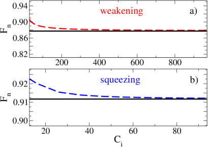
Figure 2: (color online) Limited efficiency on pure squeezing and weakening techniques. For a completely loaded initial trap ($N_{i}=C_{i}$) of depth $U_{i}=C_{i}^{2}\pi^{2}$, the resolution of a given bound state of the final trap, $\varphi_{n}^{f}$ ($n=5$, $U_{f}=25\pi^{2}$), is quantified by the measure $F_{n}=\langle\varphi_{n}^{f}|\hat{\Lambda}_{i}|\varphi_{n}^{f}\rangle$, and shown to be limited in a) pure squeezing, and b) pure weakening. For increasing capacity of the initial trap, $C_{i}$, $F_{n}$ tends to the probability to find the particle in the well region $[0,L_{i}]$ (weakening case, solid line, see Eq. (17)), or to the probability to find the particle in a momentum space region (squeezing case, solid line, see Eq.(18)).

IV Trap squeezing

There is a simple alternative to trap weakening to achieve high-fidelity Fock states: atom-trap squeezing. Starting with a state of an unknown number of particles $N_{i}$, the trap width is reduced from an initial value $L_{i}$ to $L_{f}$ keeping the depth constant ($V_{i}=V_{f}$), as shown in Fig. 1 (middle panel). The final trap supports $C_{f}$ bound states so that the excess of atoms is squeezed out of the trap. From a comparison of initial and final energy levels, it is clear that a minimum number of initial particles is required for trap squeezing to work. Using for an estimate the levels of the infinite well we get $N_{i}>C_{f}L_{i}/L_{f}$. Trap squeezing works optimally for initial traps filled with atoms to the brim but it is not robust against partial filling. It is also less sensitive to threshold effects than trap weakening, in particular for low atom numbers.

For a wide, filled initial trap,

$$\widehat{\Lambda}_{i}\sim\int_{0}^{\kappa}{\rm d}k|k^{+}\rangle\langle k^{+}|$$ (18)

as $L\to\infty$, where $\langle x|k^{+}\rangle=\sqrt{2/\pi}\sin kx$, $x\geq 0$, satisfying $\langle k^{+}|k^{\prime+}\rangle=\delta(k-k^{\prime})$ and the cut-off is at $\kappa\simeq U_{i}^{1/2}/L_{i}$, in terms of the dimensionless parameter $U_{i}=2mL_{i}^{2}V_{i}/\hbar^{2}$ ($U_{f}$ is defined similarly in terms of the final values). This is illustrated in Fig. 2b. Therefore, trap squeezing may limit the fidelity of the final Fock state preparation due to the truncation of the tails “in momentum space”, in the sense of Eq. (18), for $k>U_{i}^{1/2}/L_{i}$.

V Combined weakening and squeezing

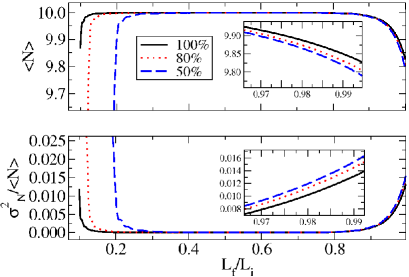
Figure 3: (color online) Asymptotic mean value (up) and variance (down) of the atom number distribution of a Tonks-Girardeau gas obtained by sudden trap reduction as a function of the width ratio between the final and initial trap. The initial trap with $U_{i}/\pi^{2}=10^{4}$ supports a maximum of $C_{i}=100$ bound states, while the final configuration $U_{f}/\pi^{2}=10^{2}$ is limited to $C_{f}=10$. Different filling factors are considered for the initial trap. The left and right edges of each curve correspond to pure squeezing and weakening respectively, the later being remarkably less sensitive to the trap filling as shown in the inset. Any other point combines weakening and squeezing.

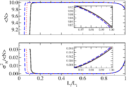
Figure 4: (color online) Asymptotic mean value (up) and variance (down) of the atom number distribution of a Tonks-Girardeau gas obtained by a sudden change of the trap potential for $U_{i}/\pi^{2}=10^{4}$ (solid line), $2.25\times 10^{4}$ (dotted line) and $4\times 10^{4}$ (dashed line) keeping a constant initial filling factor of $90\%$. $U_{f}/\pi^{2}=10^{2}$ with $C_{f}=10$. The high-efficiency region increases with $U_{i}$ reducing the critical ratio between the final and initial trap widths $L_{f}^{c}/L_{i}$.

From the previous discussion it follows that the optimal potential trap change to fullfill $\widehat{\Lambda}_{f}\subset\widehat{\Lambda}_{i}$ is a combination of weakening and squeezing. Let us choose two different families of isospectral traps characterized by $U_{i}$ and $U_{f}$, supporting $C_{i}$ and $C_{f}$ bound states respectively (In general $C_{i}>N_{i}$ because of partial filling of the initial trap, the filling factor being the ratio $N_{i}/C_{i}$). The energy level of the highest occupied state measured from the bottom of the trap, analogous to the Fermi level in the dual system, is denoted by $\varepsilon_{i}$, which depends on the filling factor of the $U_{i}$-trap, while for the ideal final Fock state $\varepsilon_{f}\simeq V_{f}$.

From an arbitrary potential $(L_{i},V_{i})$ in the $U_{i}$-family, the efficiency of the weakening-squeezing combination leading to a potential of the $U_{f}$ family varies with the filling factor and with the ratio of widths in the final and initial trap $L_{f}/L_{i}$. Figure 3 shows both the mean atom number and variance of the final states for different ratios and preparation states. Below a critical final width $L_{f}^{c}=(U_{f}/U_{i})^{1/2}L_{i}$, the physical final depth $V_{f}$ is larger than the initial one $V_{i}$ and we disregard this possibility since the efficiency is very poor as expected from the failure of the condition (16) for $\varepsilon_{f}>\varepsilon_{i}$. The ratio $L_{f}/L_{i}=1$ is the limit of pure trap weakening, and $L_{f}^{c}/L_{i}$ that of pure trap squeezing; the limited efficiency of both extreme cases can be noticed in Fig. 3. However, the combined process achieves pure Fock states and is robust with respect to different fillings in the initial trap and for a wide range of final configurations. Moreover, the range of final configurations for which high-fidelity states are obtained increases with the initial potential $U_{i}$ keeping the filling constant as shown in Fig. 4. Hence, a recipe to create a Fock state $|C_{f}\rangle$ in a trap of width $L_{f}$ and depth $V_{f}$ will be as follows: choose the width of the initial trap broad enough in the sense $L_{i}\simeq L_{f}+r\xi$ ($r\gtrsim 1$), where $\xi$ is the penetration length of the state $\varphi_{C_{f}}^{f}$ in the final trap. Then, make sure that $\varepsilon_{i}>\varepsilon_{f}$, in such a way that the final state is contained in the initial subspace both in momentum and coordinate space. A deep and broad initial trap, with respect to the final one, provides in summary a safe starting point to create a Fock state by sudden (or otherwise) trap reduction.

VI Discussion and conclusion

In this work we have studied and compared strategies for atom Fock state creation in Tonks-Girardeau regime. We have shown that Fock states can be prepared even under a sudden trap-potential change. Thanks to the analysis of the atom number variance, we have determined that the key condition for Fock state creation is that the initial occupied bound states span the space of the final ones. This holds regardless of the trap shape details, and in particular does not depend on the potential-trap model. A combination of trap weakening and squeezing allows to resolve the ideal Fock state both in momentum and coordinate space. We close by noting that the Tonks-Girardeau regime is optimal with respect to the strength of interactions. In this regime, the three-body correlation function $g_{3}(\gamma)$ tends to vanish and therefore the losses of atoms from the trap by inelastic collisions are negligible GS03 . For gases with finite interactions in tight-waveguides, when the Lieb-Liniger model holds, the quasimomenta obtained as solution of the Bethe equations Gaudin71 ; Cazalilla02 ; BGOL05 ; chinos , are closer to each other for weaker interatomic interactions, whence it follows that the required time scale for the dynamics to be adiabatic is even larger than in the Tonks-Girardeau regime. Large spacings in the Bethe roots also imply that less precision is required in the control of $V_{f}$. Given that the interatomic interactions can be tuned through the Feschbach resonance technique, one can optimize the atom Fock state preparation by putting the system within a strong interaction regime in a first stage, followed by the controlled reduction of the potential trap (weakening and squeezing), and finally turning off slowly the interaction.

Appendix A

In this appendix we describe the spectrum of the Hamiltonian for the potential in Eq. (10) considered in the numerical examples. Both the initial and final traps have the same functional dependence. Here we consider the general case for a trap of width $L$ and depth $V$ (dropping the index $\alpha=i,f$ for compactness), whose spectrum can be easily determined using matching conditions in the wavefunction and its derivatives. The trap supports a finite set of $C$ bound states (its capacity)

$$\varphi_{j}(x)=\mathcal{N}_{j}\left\{\begin{array}[]{l l}\sin(q_{j}x)&,\;\;0\leq x<L\\[7.11317pt] \sin(q_{j}L)e^{-\kappa_{j}(x-L)}&,\;\;x\geq L\end{array}\right.$$ (21)

with $j=1,\dots,C$ and normalization constant

$$\mathcal{N}_{j}=\left(\frac{L}{2}-\frac{\sin(2q_{j}L)}{4q_{j}}+\frac{\sin^{2}(q_{j}L)}{2\kappa_{j}}\right)^{-1/2}.$$ (22)

The eigenvalues are $E_{j}=(\hbar q_{j})^{2}/2m-V<0$ where $\{q_{j}\}$ satisfy the trascendental equation $\kappa_{j}=-q_{j}\cot q_{j}L$, with $\kappa_{j}=(2mV/\hbar^{2}-q_{j}^{2})^{1/2}>0$. The scattering states have the form

$$\chi_{k}(x)=\frac{1}{\sqrt{2\pi}}\left\{\begin{array}[]{l l}A\sin qx&,\;\;0<x\leq L\\[7.11317pt] e^{-ikx}-S(k)e^{ikx}&,\;\;x>L\end{array}\right.,$$ (25)

where $q=\sqrt{k^{2}+2mV/\hbar^{2}}$ and the coefficient $A$ and the scattering matrix $S(k)$ are determined by imposing the usual matching conditions,

$$A = -\frac{2ike^{-ikL}}{q\cos qL-ik\sin qL},$$

$$S(k) = e^{-2ikL}\frac{q\cos qL+ik\sin qL}{q\cos qL-ik\sin qL}.$$ (26)

References

- (1) J. Sebby-Strabley, B. L. Brown, M. Anderlini, P. J. Lee, W. D. Phillips, and J.V. Porto, Phys. Rev. Lett. 98, 200405 (2007).
- (2) A. del Campo, F. Delgado, G. García-Calderón, J. G. Muga, and M. G. Raizen, Phys. Rev. A 74, 013605 (2006).
- (3) D. Jaksch, H.-J. Briegel, J. I. Cirac, C.W. Gardiner, and P. Zoller, Phys. Rev. Lett. 82, 1975 (1999); T. Calarco, E. A. Hinds, D. Jaksch, J. Schmiedmayer, J. I. Cirac, and P. Zoller, Phys. Rev. A 61, 022304 (2000); E. Andersson and S. M. Barnett, Phys. Rev. A 62, 052311 (2000); A. M. Dudarev, R. B. Diener, B. Wu, M. G. Raizen, and Q. Niu, Phys. Rev. Lett. 91, 010402 (2003).
- (4) C. Orzel, A. K. Tuchman, M. L. Fenselau, M. Yasuda, and M. A. Kasevich, Science 291, 2386 (2001).
- (5) D. J. Wineland, J. J. Bollinger, W. M. Itano, F. L.Moore, and D. J. Heinzen, Phys. Rev. A 46, R6797 (1992); J. Hald, J. L. Sorensen, C. Schori, and E. S. Polzik, Phys. Rev. Lett. 83, 1319 (2000); A. Kuzmich, L. Mandel, and N. P. Bigelow, Phys. Rev. Lett. 85, 1594 (2000).
- (6) K. R. Brown, K.M. Dani, D.M. Stamper-Kurn, and K.B. Whaley, Phys. Rev. A 67, 043818 (2003).
- (7) M. Holland and K. Burnett, Phys. Rev. Lett. 71, 1355 (1993); J. J. Bollinger, W. M. Itano, D. Wineland, and D. J. Heinzen, Phys. Rev. A 54, R4649 (1996); P. Bouyer and M. A. Kasevich, Phys. Rev. A 56, R1083 (1997).
- (8) S. Leslie, N. Shenvi, K.R. Brown, D.M. Stamper-Kurn, and K.B. Whaley, Phys. Rev. A, 69, 043805 (2004).
- (9) C.-S. Chuu, F. Schreck, T. P. Meyrath, J. L. Hanssen, G. N. Price, and M. G. Raizen, Phys. Rev. Lett. 95, 260403 (2005).
- (10) A. M. Dudarev, M. G. Raizen, and Q. Niu, Phys. Rev. Lett. 98, 063001 (2007).
- (11) E. H. Lieb and W. Liniger, Phys. Rev. 130, 1605 (1963).
- (12) M. Olshanii, Phys. Rev. Lett. 81, 938, (1998); V. Dunjko, V. Lorent, and M. Olshanii, ibid 86, 5413 (2001).
- (13) D. S. Petrov, G. V. Shlyapnikov, and J. T. M. Walraven, Phys. Rev. Lett. 85, 3745, (2000).
- (14) K. V. Kheruntsyan, D. M. Gangardt, P. D. Drummond, and G. V. Shlyapnikov, Phys. Rev. Lett. 91, 040403 (2003).
- (15) B. Paredes, A. Widera, V. Murg, O. Mandel, S. Fölling, I. Cirac, G. V. Shlyapnikov, T. W. Hänsch, and I. Bloch, Nature (London) 429, 227 (2004); T. Kinoshita, T. Wenger, and D. Weiss, Science 305, 1125 (2004).
- (16) M. Girardeau, J. Math. Phys. 1, 516, (1960).
- (17) T. P. Meyrath, F. Schreck, J. L. Hanssen, C-S. Chuu, and M. G. Raizen, Phys. Rev. A R71, 041604 (2005).
- (18) T. Cheon and T. Shigehara, Phys. Rev. Lett. 82, 2536 (1999).
- (19) M. D. Girardeau and E. M. Wright, Phys. Rev. Lett. 84, 5691 (2000).
- (20) M. D. Girardeau, E. M. Wright, and J. M. Triscari, Phys. Rev. A 63, 033601 (2001).
- (21) W. Hänsel, P. Hommelhoff, T.W. Hänsch, and J. Reichel, Nature 413, 498 (2001).
- (22) J. Reichel and J. H. Thywissen, J. Phys. IV 116, 265 (2004).
- (23) S. L. Cornish, N. R. Claussen, J. L. Roberts, E. A. Cornell, and C. E. Wieman, Phys. Rev. Lett. 85, 1795 (2000).
- (24) The effect of the shape of the potential will be discussed elsewhere.
- (25) The probability amplitude under the barrier decays exponentially in a length scale where , see the appendix.
- (26) J. R. Taylor, Scattering Theory (Wiley, New York, 1972).
- (27) N. Bleistein and R. A. Handelsman, Asymptotic expansions of integrals (Dover, New York, 1986).
- (28) D. M. Gangardt and G. V. Shlyapnikov, Phys. Rev. Lett. 90, 010401 (2003).
- (29) M. Gaudin, Phys. Rev. A 4, 386 (1971).
- (30) M. A. Cazalilla, Europhys. Lett. 59, 793 (2002); M. A. Cazalilla, J. Phys. B 37, S1 (2004).
- (31) M. T. Batchelor, X. W. Guan, N. Oelkers and C. Lee, J. Phys. A 38, 7787 (2005).
- (32) Y. Hao, Y. Zhang, J.-Q. Liang, and S. Chen, Phys. Rev. A 73, 063617 (2006).