Detection of transplanckian effects in the cosmic microwave background

Abstract

Quantum gravity effects are expected modify the primordial density fluctuations produced during inflation and leave their imprint on the cosmic microwave background observed today. We present a new analysis discussing whether these effects are detectable, considering both currently available data and simulated results from an optimal CMB experiment. We find that the WMAP data show no evidence for the particular signature considered in this work, but give an upper bound on the parameters of the model. However, a hypothetical experiment shows that with proper data, the transplanckian effects should be detectable through alternate sampling methods. This fuzzy conclusion is a result of the nature of the oscillations, since they give rise to a likelihood hyper-surface riddled with local maxima. A simple Bayesian analysis shows no significant evidence for the simulated data to prefer a transplanckian model. Conventional Markov Chain Monte Carlo (MCMC) methods are not suitable for exploring this complicated landscape, but alternative methods are required to solve the problem. This however requires extremely high-precision data.

I Introduction

Quantum fluctuations in the scalar field responsible for driving inflation can give rise to a power spectrum of primordial density perturbations consistent with what is required to seed the large-scale structure (LSS) and the temperature anisotropies in the cosmic microwave background (CMB) radiation. This fact is probably one of the main reasons for inflation having become a part of the concordance model of cosmology today. The quantum fluctuations are imprinted during the early inflationary epoch, and become classical fluctuations in the gravitational potential as the fluctuations leave the causal horizon. The standard way of calculating the power spectrum of the density fluctuations make use of the fact that space-time becomes Minkowskian in the distant past. However, it has been argued Martin and Brandenberger (2001); Easther et al. (2001); Danielsson (2002, 2006); Martin and Ringeval (2004a, 2006, b, 2005); Bergström and Danielsson (2002) that since a given length scale observable in the universe today shrinks and becomes smaller than the Planck length if followed sufficiently far back in time, effects of quantum gravity will at some point play a role in setting up the perturbations, and may potentially leave an observable signature. The primordial density fluctuations in the early universe may have small oscillations superimposed as a result of quantum gravitational effects. These effects are due to non-negligible curvature imposed by high energy densities in de Sitter space during the early stages of inflation. Several papers have suggested a generic shape of these effects Danielsson (2002, 2006); Bergström and Danielsson (2002) in the form of small oscillations superimposed on the standard, nearly scale-invariant primordial power spectrum of density fluctuations. A crucial questions is, of course, whether such a signature is observable in the universe today. This question has been investigated in several papers Martin and Ringeval (2004a, 2006, b, 2005); Elgarøy and Hannestad (2003); Danielsson (2002, 2006). The conclusion in Elgarøy and Hannestad (2003) was pessimistic: the so-called transplanckian effects were found to be unobservable in practice. However, this conclusion has been called into question in Martin and Ringeval (2005). One of the problems pointed out in that work is that the oscillations require more numerical accuracy than what is commonly employed in codes like CMBFAST Seljak and Zaldarriaga (1996) and CAMB Lewis et al. (2000).

In this paper, we revisit the question of the observability of transplanckian effects in the CMB, using a more accurate numerical treatment than in Elgarøy and Hannestad (2003). Both present data and a hypothetical optimal CMB experiment are considered. Furthermore, we mention alternative sampling algorithms to overcome the numerical problems encountered in exploring what turns out to be a particularly nasty likelihood hyper-surface. Section II gives a brief description of the particular model we consider and the data sets we use. In section III we discuss some technical details in the numerical computations undertaken. Section IV then contains results obtained with currently available data sets, and in section V we investigate the possibilities with an ideal CMB data set. The exact likelihood function is described in section VI, while a Bayesian evidence analysis is performed in section VII. A discussion of the results and a suggestion for an improved approach to the search for transplanckian effects can be found in section VIII, and we conclude in section IX.

II Background

Neglecting the perturbations in the metric during inflation, it is viable to assume that the inflaton scalar field can be expressed as:

$$\phi(\textbf{x},t)=\underbrace{\phi_{0}(t)}_{\text{classical evolution}}+\underbrace{\delta\phi(\textbf{x},t)}_{\text{fluctuations}}$$ (1)

The fluctuations in a scalar field $\delta\phi$ in a Friedmann-Lemaître-Robertson-Walker background satisfy the equation of motion (EOM):

$$\ddot{\delta\phi}+3H\dot{\delta\phi}-\frac{1}{a}(\nabla^{2})\delta\phi+m^{2}\delta\phi=0$$ (2)

where the dot denotes the derivative with respect to time and $m^{2}\propto d^{2}V/d\phi^{2}$, where $V(\phi)$ is the inflaton potential. Performing a Fourier expansion of the fluctuations:

$$\delta\phi(x,t)=\frac{1}{\sqrt{N}}\sum_{k}u_{k}(t)e^{ikx}$$ (3)

where $N$ is a normalization constant, equation (2) becomes:

$$\ddot{u}_{k}+3H\dot{u}_{k}+(\frac{k^{2}}{a^{2}}+m^{2})u_{k}=0.$$ (4)

Assuming de Sitter space, this equation can be rewritten using a change of variable ($u_{k}\equiv\varphi/a$) and switching to conformal time ($d\eta=dt/a$). This removes the friction term, and the final EOM becomes:

$$\varphi_{k}^{\prime\prime}+\Big{(}k^{2}-\frac{2}{\eta^{2}}\Big{)}\varphi_{k}=0$$ (5)

where ^′ denotes derivative with respect to conformal time $\eta$. A detailed derivation of this result can be obtained in Dodelson (2003). The general solution for $\varphi_{k}$ is:

$$\varphi_{k}=\frac{A_{k}}{\sqrt{2k}}e^{-ik\eta}\Big{(}1-\frac{i}{k\eta}\Big{)}+\frac{B_{k}}{\sqrt{2k}}e^{ik\eta}\Big{(}1+\frac{i}{k\eta}\Big{)}$$ (6)

where $A_{k}$ and $B_{k}$ are Bogoliubov coefficients satisfying $|A_{k}|^{2}-|B_{k}|^{2}=1$, $\eta$ is the conformal time and $k$ is the wave mode. The usual choice of vacuum is the Bunch-Davies vacuum, which corresponds to $A_{k}=1$ and $B_{k}=0$. Space-time becomes Minkowskian in the infinite past ($\eta\to-\infty)$, where it is feasible to impose initial conditions on the field equations.

In Danielsson (2006), different possibilities for suitable vacua are discussed before focusing on a specific choice, the adiabatic vacuum, for which $a_{k}(\eta_{0})|0,\eta_{0}\rangle=0$. This vacuum (for a given $\eta_{0}$) is a typical representative of vacua, and corresponds to a minimum uncertainty between field and its conjugate momentum Polarski and Starobinsky (1996). When imposing initial conditions, Bogoliubov-coefficients are constrained by the relation Danielsson (2006):

$$B_{k}=\frac{ie^{-2ik\eta_{0}}}{2k\eta_{0}+i}A_{k}.$$ (7)

Note that the Bunch-Davies vacuum is restored in the infinite past: When $\eta_{0}\to-\infty$, $A_{k}=1$ and $B_{k}=0$. A discussion of the implications of the choice of vacuum can be found in Bozza et al. (2003); Campo et al. (2007).

When choosing this zeroth order adiabatic vacuum Danielsson (2002), the primordial curvature spectrum can be expressed as Danielsson (2006):

$$P(k)=\Big{(}\frac{H}{\dot{\phi}}\Big{)}^{2}\Big{(}\frac{H}{2\pi}\Big{)}^{2}\Big{(}1-\frac{H}{\Lambda}\sin\big{(}\frac{2\Lambda}{H}\big{)}\Big{)}$$ (8)

where $\Lambda$ is the (Planck) energy cutoff scale and $H$ the Hubble parameter. Note that the size of the corrections is linear Kaloper et al. (2002) in $H/\Lambda$. In Kaloper and Kaplinghat (2003), it is argued that equation (8) represents a generic effect, regardless of the details in the (undetermined) transplanckian physics. In Danielsson (2006), equation (8) is further parametrized as

$$P(\epsilon,\xi,k)=P_{0}(k)\Big{(}1-\xi\Big{(}\frac{k}{k_{n}}\Big{)}^{-\epsilon}\sin\Big{[}\frac{2}{\xi}\Big{(}\frac{k}{k_{n}}\Big{)}^{\epsilon}\Big{]}\Big{)}$$ (9)

with variables explained in table 1.

Parameter	Value	Description
$\epsilon$	$\epsilon\ll 1$	The slow roll parameter
$\gamma$	$\Lambda/M_{pl}$	The transplanckian scale
$M_{pl}$	$1/\sqrt{8\pi G}$	The reduced Planck mass
$\xi$	$4\cdot 10^{-4}\frac{\sqrt{\epsilon}}{\gamma}$	A parametrization of $H/\Lambda$
$k_{n}$	$k_{n}$	The largest measurable scale
$P_{0}(k)$	$\propto k^{n_{s}-1}$	The standard power spectrum

Table 1: Explaining equation (9)

Notice how the standard inflationary power spectrum $P_{0}$ is restored as the cutoff $\xi\propto\frac{1}{\Lambda}\to 0$. It is also interesting to note that for low cutoff values $\xi\propto\frac{1}{\Lambda}\to\infty$, the amplitude of the modulation converges to $2$ (as $\lim_{x\to\infty}x\sin(2/x)=2$). The amplitude of the oscillations never reaches values greater than $2$, and only severely impacts $P_{0}$ for large values of $\xi$. Physically, if the cutoff $\xi\propto\frac{1}{\Lambda}$ was enforced at low values (large $\xi$), it should easily be detectable in the the cosmic microwave background, as will be presented in the following section. This is, however, not the case, and we know that the transplanckian physics leave imprints at $\xi\ll 1$, corresponding to a cutoff at high energies. The amplitude of the oscillations is therefore expected to be very small.

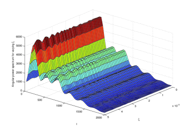
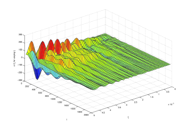
When evolving the modulated primordial power spectrum through CAMB, the transplanckian imprints for varying $\xi$ in the full power spectrum can be seen in figure 1. The oscillations singled out for varying $\xi$ are presented in figure 2.

Figure 1: The full power spectrum $C_{\ell}$ for varying $\xi$.

Figure 2: The transplanckian modulations $\Delta C_{\ell}$ for varying $\xi$.

II.1 A brief summary of recent results

Reference Danielsson (2002) concludes that effects of transplanckian physics are possibly within the reach of cosmological observations. Equation (9) describes a a generic expression for how transplanckian effects would modify the primordial power spectrum. As seen in the previous section, these oscillations are caused by a nontrivial vacuum for the inflaton field Danielsson (2002, 2006). As the oscillations are expected to contribute to the energy density, this could change the way the universe expands, and in a worst-case scenario, the inflationary phase could be destroyed. The authors of Danielsson (2006) investigate this possibility, and conclude that the the back reaction is under control and fully consistent with inflation, with a slow roll found to be completely dominated by the vacuum energy given the parameters suggested in Martin and Ringeval (2006).

II.1.1 WMAP data and transplanckian effects

A previous data analysis Brandenberger (2001) concluded that no significant signals from transplanckian effects are visible in the CMB. Another analysis Martin and Ringeval (2006) claimed that there are some weak hints in the current data, and these indications have become slightly stronger with the WMAP3 data compared to earlier claims by the same authors Martin and Ringeval (2004a, 2006, b, 2005). The parameters implied by the data suggests oscillations in amplitude that are periodic in the logarithm of the scale of the CMB fluctuations, just as predicted from transplanckian physics.

In Martin and Ringeval (2004a), the authors discuss the so-called cosmic variance outliers, i.e. points which lie outside the $1\sigma$ cosmic variance error. These outliers are considered interesting as the probability of their presence is very small Spergel et al. (2007). The authors mention that it has been envisaged that the outliers could be a signature of new physics, even though the cosmic variance could be responsible for their presence. The conclusion of Martin and Ringeval (2004a) is that there exist statistical justification for a presence of oscillations in the power spectrum. It should however be noted that the authors of Martin and Ringeval (2004a) treat the amplitude of the oscillations as a free parameter, which ensures the fitting of the cosmic variance outliers with the transplanckian oscillations.

Another paper Elgarøy and Hannestad (2003) was less optimistic, and concluded that it is unlikely that a transplanckian signature of this type can be detected in CMB and large-scale structure data. However, Elgarøy and Hannestad (2003) left some technical issues open, and we find it worthwhile to revisit this problem. We show that the current WMAP3 data gives weak constraints on the parameters of the transplanckian model using conventional MCMC methods.

II.1.2 Simulated data and transplanckian effects

The conclusion of Elgarøy and Hannestad (2003) was that CMB and LSS data are in principle sensitive to transplanckian modulations in the primordial power spectrum, but that is practically impossible to make a positive detection even in future high-precision data. This has to do with the nature of the oscillations, as the value of the likelihood function is extremely sensitive to $\epsilon$ and $\xi$. But what “extremely sensitive” means was not explained in Elgarøy and Hannestad (2003). We will show explicit examples of how this sensitive likelihood function contemplates trouble, and why this renders the underlying MCMC method in CosmoMC of little use in estimating the transplanckian parameters.

III Numerical details

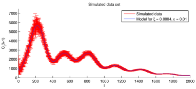
CAMB Lewis et al. (2000) was modified to include the primordial oscillations described in equation (9), adding the parameters $\xi$ and $\epsilon$. Based on a power spectrum generated using the modified version of CAMB, a $TT$ data set was simulated by drawing from a $\chi^{2}$-distribution with $2\ell+1$ degrees of freedom. The data set and model are depicted in figure (3), and the choice of values for $\xi=0.0004$ and $\epsilon=0.01$ are motivated by the Horava-Witten model Horava and Witten (1996) of transplanckian physics Danielsson (2006). In this model, unification occurs at the scale where a fifth dimension becomes visible Kaloper et al. (2002), resulting in quite optimistic estimates of the energy scale where quantum gravity effects are manifested. However, the oscillations for this low value of $\xi$ corresponds to very small superimposed oscillations in the primordial power spectrum, as seen from figure 1 and 2. The remaining cosmological parameters used for creating the data set (eg $\Omega_{b},\tau,n_{s}$) were chosen as $\Lambda CDM$ best-fit values. We continued by creating a simulated $TE,EE$ and $BB$ data set using the same methods described here.

Figure 3: Simulated $TT$ data based on $\xi=0.0004$ and $\epsilon=0.01$.

The MCMC software package CosmoMC Lewis and Bridle (2002) was altered to include the parameters $\xi$ and $\epsilon$. Based on the likelihood for ideal noiseless simulated data described in Verde et al. (2003), the WMAP-likelihood code of CosmoMC was adjusted to utilize the ideal data instead of the WMAP 3-year data. The TT-only likelihood function is given by

$$-2\log\mathcal{L}(x_{i};p_{i})=\sum_{\ell}(2\ell+1)\Big{[}\ln\big{(}\frac{C_{\ell}}{\hat{C}_{\ell}}\big{)}+\frac{\hat{C}_{\ell}}{C_{\ell}}-1\Big{]}.$$ (10)

where $C_{\ell}$ are the theoretical TT power spectra and $\hat{C}_{\ell}$ TT data sets. The same method for creating and using ideal data with CosmoMC was employed in Mota et al. (2007). The errors in this ideal data set are only limited by cosmic variance, so no experiment can give any better estimate of the power spectrum. Thus, if transplanckian effects are not detectable in the simulated data, they cannot be detectable with any future high-precision data. We continued by employing the full simulated $TT,TE,EE$ and $BB$ data set using the likelihood presented in Easther et al. (2005):

$$-2\ln\mathcal{L}=\sum_{\ell}(2\ell+1)\Big{[}\ln\big{(}\frac{C_{\ell}^{BB}}{\hat{C}_{\ell}^{BB}}\Big{)}+\ln\big{(}\frac{C_{\ell}^{TT}C_{\ell}^{EE}-(C_{\ell}^{TE})^{2}}{\hat{C}_{\ell}^{TT}\hat{C}_{\ell}^{EE}-(\hat{C}_{\ell}^{TE})^{2}}\Big{)}$$ (11)

$$+\frac{\hat{C}_{\ell}^{TT}C_{\ell}^{EE}+C_{\ell}^{TT}\hat{C}_{\ell}^{EE}-2C_{\ell}^{TE}\hat{C}_{\ell}^{TE}}{C_{\ell}^{TT}C_{\ell}^{EE}-(C_{\ell}^{TE})^{2}}$$ (12)

$$+\frac{\hat{C}_{\ell}^{BB}}{C_{\ell}^{BB}}-3\Big{]}$$ (13)

III.1 Increasing accuracy

Figure 4: The ratio of modulated power spectrum with low and high accuracy, all 3 parameters boosted.

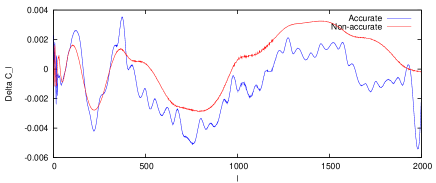
Previous papers Martin and Ringeval (2004b, 2005) have pointed out that it is necessary to increase the accuracy of the calculated power spectrum used for estimating the transplanckian parameters. The results in Elgarøy and Hannestad (2003) might therefore have been partly due to the inaccuracy in the version of CMBFAST Seljak and Zaldarriaga (1996) used in this work. The accuracy of the numerical calculations was boosted, which increased run time by a tenfold. The results can be seen in figure 4. However, the accuracy boosting had little or no effect on the WMAP parameter estimation, as will be explained in the following section.

IV Results from WMAP3 data

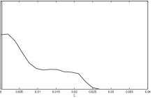
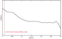
For small values of the transplanckian values, the constraints on both $\xi$ and $\epsilon$ from the WMAP3 data turned out rather poor when running CosmoMC with all standard cosmological parameters free. This can be seen in figure 5 and 7, consistent with the results in Elgarøy and Hannestad (2003). For larger values of the transplanckian parameter $\xi$, the increasing amplitude of the primordial power spectrum effectively constraints $\xi$ to the interval $[0,0.02]$ (recall from section II that for large $\xi$, the amplitude converges to $2$). This can be seen in figure 6. This corresponds to a cutoff $\Lambda\sim 0.002M_{pl}\sim 10^{16}GeV$. Everything below this scale ($\xi>0.02$) should therefore be ruled out by WMAP3 data.

Figure 5: Marginalized posterior for $\xi$ over a small interval surrounding the original input parameter $\xi=0.0004$ from the Horava-Witten model (red line).

Figure 6: Marginalized posterior of $\xi$ over a larger interval. The red line corresponds to $\xi=0.0004$ from the Horava-Witten model. Notice how it is possible to estimate an upper bound: $\xi_{max}\sim 0.02$. Above this threshold, there are occasional “bumps” in the posterior where the oscillation reaches zero ($\sin x=0$, see equation 9).

Figure 7: Marginalized posterior for $\epsilon$. The red line corresponds to $\epsilon=0.01$ from the Horava-Witten model.

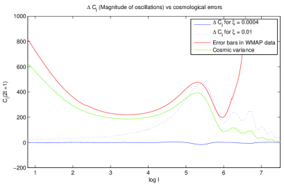
For physically reasonable values of $\xi$ and $\epsilon$ ($\ll 1$), the amplitude of the modulations are well below $1\%$ of the total power spectrum. Also, the cosmic variance and the errors in the WMAP data are several orders of magnitude greater than the amplitude of the modulations in the power spectrum, as can be seen from figure 8. This explains why any detection of transplanckian effects in the WMAP data fails for low values of $\xi$.

Figure 8: The blue line shows the oscillations $\Delta C_{\ell}$ in the primordial power spectrum for $\xi=0.0004$, $\gamma=0.01$ and $\epsilon=0.01$. The red bars are the error bars in the WMAP data, while the green graph is the cosmic variance. Notice how the modulations in the low-$\xi$ power spectrum (blue line) are much smaller than either. The dotted blue line represents a larger $\xi\sim 0.01$, which should be possible to detect, and gives upper constraints on $\xi$.

V Results from ideal CMB data

Figure 9: Top left: Marginalized posterior for $\xi$ with mean value at $0.978\cdot 10^{-3}$. Top right: Marginalized posterior for $\xi$ with mean value at $0.515\cdot 10^{-3}$. Bottom left: Marginalized posterior for $\xi$ with no peak, almost uniform distribution. Bottom right: Marginalized posterior for $\xi$ with several peaks. Notice how the peaks don’t match, where the red line represents the Horava-Witten input parameter $\xi=0.0004$ for the simulated data.

The WMAP3 data in CosmoMC was replaced by the optimal data set created from the power spectrum based on the Horava-Witten model. The ideal $TT$ data are shown in figure 3.

V.1 Simulated TT data

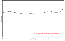
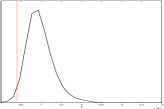
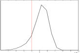
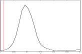
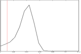
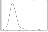
When performing parameter estimation of the transplanckian parameters $\xi$ and $\epsilon$ using the $TT$-data setup, the Monte Carlo Markov chain-method failed to converge to a stationary distribution. The resulting likelihoods for various $\xi$ and $\epsilon$ are presented in figure 9 and 10, respectively. Notice how different initial conditions and varying step length affect the end result: different initial parameters for the same parameter results in different distributions. This suggests that the likelihood function which decides the path of the random walkers traversing the cosmological parameter space has some troublesome properties.

Figure 10: Top left: Marginalized posterior for $\epsilon$ with mean value at $0.12$. Top right: Marginalized posterior for $\epsilon$ with mean value at $0.037$. Bottom left: Marginalized posterior for $\epsilon$ with mean peak at $0.101$. Notice how the peaks do not agree for different step lengths, where the red line represents the Horava-Witten input parameter $\epsilon=0.01$ for the simulated data.

V.2 Simulated TT,TE,EE and BB data

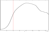
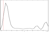
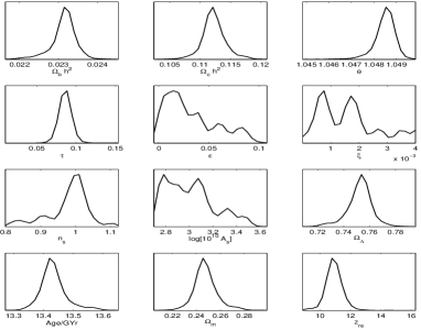
The marginalized posteriors can be seen in figure 11. Notice how $\tau$ is restored due to the inclusion of simulated TE and EE data. The transplanckian parameters now reflect the ruggedness of the likelihood-function, and traces can also be seen in $n_{s}$ and $A_{s}$. As in the TT-case, the original transplanckian input parameters are still not possible to pin down.

Figure 11: Marginalized posteriors for the full TT, TE, EE and BB likelihood analysis using equation (11)

Figure 12: Marginalized posteriors (red lines) with smaller bins than in figure 11 for the full TT, TE, EE and BB likelihood analysis using equation (11). The likelihoods are depicted with blue lines. Notice how the posteriors completely failed to converge to a distribution.

Figure 11 and 12 show how the MCMC process fails in converging, as the marginalized posterior show random walkers “trapped” in local minima.

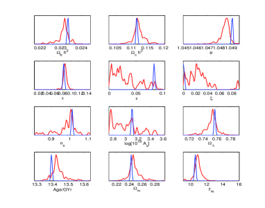
VI The exact likelihood function

In order to explain why the parameter estimation fails, we investigated the likelihood function in the case of noiseless data and different power spectra for fixed cosmological parameters except the transplanckian $\xi$ and $\epsilon$. This was done by grid integration, and no MCMC-sampling was involved. The resulting likelihood surfaces for continuous variations in $\xi$ and $\epsilon$ are seen in figure 13 and 15, respectively. A figure of the exact two-dimensional likelihood surface for both $\xi$ and $\epsilon$ is presented in figure 16. Figures 13, 14, 15 and 16 are $-\log\mathcal{L}$-plots, so the best-fit value corresponds with the global minimum. The likelihood surfaces are riddled with local minima, effectively rendering the usual MCMC-method useless: the random walkers become “trapped” in the local holes, and will have problems converging to the correct stationary distribution. Take especially note of the two-dimensional parameter space presented in figure 16, a landscape reminiscent that of an egg container.

Figure 13: $-\log\mathcal{L}$ as a function of $\xi$ for simulated transplanckian data.

Figure 14: $-\log\mathcal{L}$ as a function of $\xi$ for simulated non-transplanckian data. Notice how the non-transplanckian data is preferred to the simulated transplanckian data set.

Figure 15: $-\log\mathcal{L}$ between varying $\epsilon$ and simulated data.

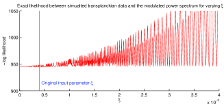
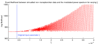
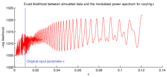
The shape of the exact likelihood is a result of the nature of the oscillations: equation (9) gives rise to a particularly nasty behaviour of the oscillations .

Figure 16: $-\log\mathcal{L}$ for varying both $\xi$ and $\epsilon$. The red ring represents the original input parameters $\xi=0.0004,\epsilon=0.01$ for the simulated data set. Notice how a random walker would be trapped in any of the other local minima.

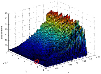
The problem with the likelihood function is not easily solved. In principle, one could perform a smoothing of the likelihood, something which works well in a low-dimensional parameter space, but is hopelessly inefficient for a realistic number of parameters.

VI.1 Decoupling the amplitude

Figure 17: -log Likelihood for varying $\xi$ and amplitude

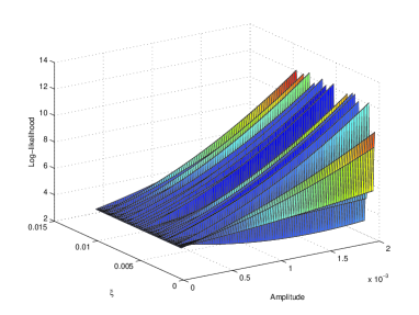
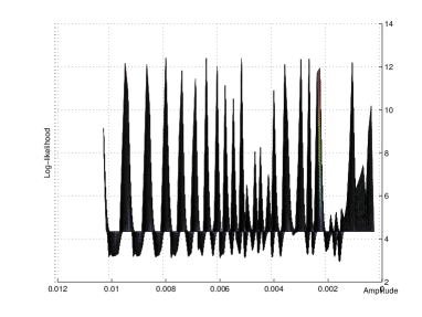
The amplitude and the frequency of the transplanckian oscillations are linked in the model we have considered so far. However, it is certainly possible that they might vary independently, and in Martin and Ringeval (2004a, 2006, b, 2005), the authors operate with the amplitude of the transplanckian oscillations as a free amplitude. We repeated our analysis with frequency and amplitude decoupled. From figure 17 and 18 it should be clear that freeing the amplitude does not really add any significance to the likelihood surface: the likelihood still gives the correct preferred amplitude.

Figure 18: -log Likelihood for varying $\xi$ and amplitude (different viewing angle)

VII Bayesian evidence

From the logarithmic likelihood in figure 13 and 15, it is obvious that it is impossible extract the values of the parameters of our model from the simulated data. However, one might still ask the question of whether the data prefer the transplanckian model to the standard power-law primordial power spectrum. In a Bayesian framework this question is answered by calculating the evidence ratio of the two models, see Mukherjee et al. (2006) for a nice introduction. Here we fix $\epsilon=0.01$ and use the evidence ratio to see whether the data prefer the introduction of the additional parameter $\xi$. We assume that the transplanckian parameter $\xi$ is not degenerate with any of the cosmological parameters, designated by the parameter vector $\theta$. This might seem like a strong assumption, but we have checked that it is reasonable for the model and the parameters we consider in this paper. Also, the effects of primordial oscillations have been investigated in Hamann et al. (2007), concluding that degeneracies of oscillations with standard cosmological parameters are virtually non-existent.

Let $\theta$ denote the non-transplanckian cosmological parameters, and $\hat{\theta}$ the best-fit $\Lambda CDM$ parameters. The logarithmic evidence is given by

$$\Delta\ln E=\ln E-\ln E^{0}$$ (14)

where $E^{0}$ is the evidence of the non-transplanckian model. Then

$$\Delta\ln E=\langle\mathcal{L}\rangle_{\pi(\theta,\xi)}-\langle\mathcal{L}\rangle_{\pi(\theta)}$$ (15)

$$=\langle\mathcal{L}(\theta,\xi)\rangle_{\pi(\xi)}-\mathcal{L}(\hat{\theta})$$ (16)

where $\pi(\theta,\xi)$ is the prior over $(\theta,\xi)$ and $\pi(\theta)$ is the prior over $\theta$. Thus, $\langle\mathcal{L}\rangle_{X}$ denotes the mean likelihood over the prior space $X$.

Figure 19: Likelihood $\mathcal{L}(\xi)$ used in calculating the significant evidence.

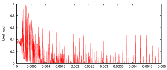
The likelihood can be found in figure 19, which is the exponential of the negative values in figure 13. We choose the prior to be $\xi\in[0,0.005]$. This results in $\Delta\ln E\approx-1.5$ which shows that the transplanckian model is slightly not preferred. Hence even perfect CMB-measurements over the whole sky does not give any significant evidence for transplanckian effects. When constraining the prior to reside in $\xi\in[0,0.0005]$, then $\Delta\ln E\approx 0.15$ and the transplanckian model is more or less equally preferable to the non-transplanckian model. This is hardly surprising, as a continuous constraint of the prior $Pr(\xi)=\lim_{\xi\to 0}[0,\xi]$ results in $\Delta\ln E=\ln E^{0}-\ln E^{0}=0$, which corresponds with the standard non-transplanckian model. The evidence never grows larger than $\sim 0.15$ for any prior constraint on $\xi$.

VIII Alternate multilevel sampling

There exists a few multilevel sampling methods besides the standard MCMC/Metropolis-Hastings algorithm that can tame the ruffled likelihood through a series of optimizations. Reference Liu (2002) contains a detailed introduction to these methods, most notably simulated annealing, umbrella sampling and the simulated tempering method. We proceed by a rough discussion on how some of these alternate sampling methods work when investigating the 1-dimensional likelihood presented in figure 13.

VIII.1 Metropolis-Hastings method, 1D

Figure 20: The posterior of 10 000 MCMC walkers evaluated after 22 000 steps each in 1 dimension, with initial conditions $\xi_{0}=0.0015$. None of the walkers reached the correct value of $\xi=0.0004$.

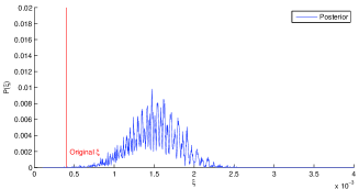
Figure 20 shows the posterior of 10 000 walkers after $\sim$ 22 000 steps each, using the Metropolis-Hastings algorithm. The likelihood is shown in figure 13. In theory, the walkers should converge to a stationary distribution with the tallest peak located at $\xi=0.0004$, but due to the ruffled likelihood this will take forever. The initial values for the walkers was here $\xi_{0}=0.0015$. This reflects what we have seen in figure 9, 10, 11 and 12 : that the complicated likelihood surface prevents the posterior to converge to the correct shape.

VIII.2 Modified Metropolis-Hastings method, 1D

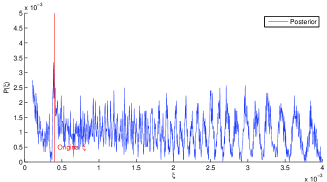
Figure 21 shows the posterior of 10 000 walkers after $\sim$20 000 steps each, using the Metropolis-Hastings algorithm. In addition, for each step there is a $0.01\%$ chance for a given walker to perform a “large” jump to a new, (uniformly) random location. The walkers will therefore tend to accumulate at the correct location (where the -log likelihood is lowest, $\xi=0.0004$). This is a slow method, and needs a fair amount of steps to give results. It is also not especially “robust”, as the accumulation of walkers at the lowest point is dependent on fine-tuning the large-step rate (here, $0.01\%$).

Figure 21: The posterior of 10 000 MCMC walkers evaluated after 22 000 steps each in 1 dimension, with initial conditions $\xi_{0}=0.0015$. The posterior shows a clear contribution around the correct value of $\xi=0.0004$.

VIII.3 Simulated annealing, 1D

Figure 22: The result of 10 000 MCMC walkers evaluated after 6 000 steps in 1 dimension, with initial conditions $\xi_{0}=0.0015$ (not a posterior). The temperature was slowly decreased until reaching $T=0$, where the correct value $\xi=0.0004$ was obtained.

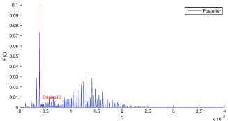
A description of the simulated annealing (SA) method can be found in Liu (2002). As in the previous examples, 10 000 random walkers were initialized at $\xi_{0}=0.0015$. The distribution spread out evenly as the SA temperature $T$ was high, and started converging to different minima as $T$ was lowered. As $T\to 0$, a good portion of walkers ended up at $\xi=0.0004$, as seein in figure 22. This shows that the SA method can be successfully used to determine the correct minima for this type of likelihood landscape.

However, the implementation and investigating of these alternative methods in CosmoMC is a major undertaking which we hope to pursue in future work.

IX Conclusion

We have shown that standard MCMC methods are not suitable for detecting transplanckian oscillations in the CMB. The 3-year WMAP3 data alone gives weak upper constraints on the transplanckian parameters. With the simulated noiseless data, the results are more ambiguous. In theory, the estimation of the transplanckian parameters should be possible, but the messy likelihood function renders conventional MCMC methods of little use. This is not due to the amplitude of the superimposed oscillations in the power spectrum alone, but rather reflects the chaotic behaviour of the oscillations for varying transplanckian parameters $\xi$ and $\epsilon$. Small variations in the parameter space thus correspond to large variations in the likelihood function, as presented in figure 13 and 15. As in Elgarøy and Hannestad (2003), we conclude that CMB data are highly sensitive to these modulations in the primordial power spectrum, but it is virtually impossible to perform a parameter estimation from WMAP3 data or high-precision simulated data using conventional MCMC methods. We have also shown, via Bayesian analysis, that even a high-precision measurement of the full CMB sky does not give any significant evidence for transplanckian effects. It should however be possible to implement the SA-method in CosmoMC when using simulated high-precision data in order to detect the transplanckian parameters.

We have in this paper shown that it is very unlikely that CMB-data could support the establishment of transplanckian effects, even for models where quantum gravity is relevant on relatively low energy scales, like in the Horava-Witten model. There are several reasons for this lamentable conclusion:

• A low quantum gravity scale, for example the value $\xi=0.0004$ chosen in our simulations, gives a very low amplitude of the oscillations in the primordial power spectrum. Hence, cosmic variance diffuses the (assumed noiseless) signal.

• Evidence can maximally rise above $0.15$, showing that the transplanckian model is only very weakly preferred when assuming a Horava-Witten universe.

• Even large (and unphysical) values of $\xi$ will result in good fits for singular points due to the behaviour of the oscillations (they periodically reach zero when $\sin x=0$)
  

• The conventional MCMC-methods in CosmoMC fails, and we have no current computational methods implemented for solving the problem of transversing the extremely complicated likelihood surface.