Systemic risk in a network fragility model analyzed with probability density evolution of persistent random walks

Abstract

We study the mean field approximation of a recent model of cascades on networks relevant to the investigation of systemic risk control in financial networks. In the model, the hypothesis of a trend reinforcement in the stochastic process describing the fragility of the nodes, induces a trade-off in the systemic risk with respect to the density of the network. Increasing the average link density, the network is first less exposed to systemic risk, while above an intermediate value the systemic risk increases. This result offers a simple explanation for the emergence of instabilities in financial systems that get increasingly interwoven. In this paper, we study the dynamics of the probability density function of the average fragility. This converges to a unique stable distribution which can be computed numerically and can be used to estimate the systemic risk as a function of the parameters of the model.

1 Introduction

1.1 Systemic Risk in Financial Networks

A network of interdependent units which, individually, are susceptible to fail, is potentially exposed to multiple joint failures of a significant fraction of units in the system. This is the notion that is usually associated with the term systemic risk. Systemic risk is particularly important in the context of infrastructure networks, such as power grids, and in financial networks. These latter should be meant in a broad sense, including units of different types, such as business firms, insurance companies, banks, mutual funds and other financial institutions that are linked by credit relationships. For instance, if one or more firms fail and are not able to pay back their debts to the bank, this affect the balance sheet of the bank which might try to improve its own situation by increasing the interest rate to the other firms, causing other failures among the firms. If finally the bank itself fails, this affects negatively the banks that are linked to it by interbank loans. This is somehow similar to failure cascades in power grids where a failing power line implies a higher load an other lines which might bring them to fail. The size distribution of such failure avalanches is one way of quantifying the systemic risk.

There is a growing body of literature in economics on financial networks, that investigates also the issue of systemic risk. While banks-firms credit relationships have been extensively studied (for an overview, see [17]), only recent works have analysed phenomena of financial contagion in interbank credit [2, 12] and trade credit. The latter, is a form of credit among business firms, typically in a supplier-customer relation, which has been less investigated despite the fact that in some countries it represents a significant part of the short-term liabilities of the corporate sector [9]. In the literature on complex networks only few works have dealt with financial networks, mainly in the context of self-organized criticality [1, 14]. Most of those works suggest that when the degree of the nodes in the network increases the network is less exposed to systemic risk. In some cases, the evidence that systemic failures may more rare but also more severe has been found (see for instance [14]).

1.2 The Fragility Model for Cascades on Networks

In this paper, we consider the model of cascades on networks introduced by [6], in which a clear tradeoff emerges in the systemic risk, as a function of the network density. This means that up to an intermediate level of network density there is a benefit in creating links between units because they allow to diversify the risk. However, above a certain level of density, the probability of many joint failures increases. This effect depends on the presence of a sort of trend reinforcing term in the dynamics of the fragility of the nodes. The fragility is a state variable that determines the failure of the node, when it exceeds a given threshold, as well as subsequent transfer of some damage to the connected nodes. The trend reinforcing of the fragility corresponds to the following idea. If the fragility of a firm at the end of the year has reduced compared to last year, the firm is rated better in terms of solvency and it has easier access to credit. Conversely, if the fragility has increased, the firm faces worse conditions for credits and thus additional cost that are likely to increase its fragility furthermore. Notice that, through the links in the network, this propagates also to the neighbours, since the fragility of the firm affects the fragility of the neighbours. For instance, hedge funds leverage even small differences in performance across firms by ’short-selling’ the stocks of the slightly worse ones and ’going long’ on the slightly better ones. Thus, even small differences in the evolution of two firms may matter a lot. Further on, effects like predatory trading [10] may induce trend reinforcing.

1.3 Outline of the Paper

In [6], some analytical results supporting the simulations are found, based on separating the process of the evolution of fragility (approximated as a time-dependent Ornstein-Uhlenbeck process) and the cascade process (where the size of an avalanche is expressed as the fix point of an equation for the number of failures). Here, we provide an alternative analysis of the tradeoff regarding systemic risk mentioned above. We consider the stochastic process defined by the mean field approximation of the fragility of the individual node. This is now a stochastic process for a single variable, and it is also clear that, having reduced the system to one single variable, the cascading part of the process is excluded by construction. In this approximation the failure probability can be taken as a proxy for systemic risk. In fact, the mean field approximation is valid when all units behave in a similar way. We study some mathematical properties of the process and we provide a simple method to show the existence of a tradeoff in systemic risk as function of the density of the network. The method is based on recognizing that the process is a combination of a Gaussian Random Walk (RW) and a Persistent Random Walk (PRW). PRW [19] is a variant of the classic RW in which the walker has a probability $p$ to keep the direction of his former movement and $1-p$ to switch direction. The process is sometimes called correlated random walk. It is approximated by the Telegraph’s equation [18, 13] in the limit of continuous time and space. It differs from RW in the scaling with time of the variance of the displacement of the walker. In our model, the dynamics in time of the fragility induces a dynamics on the probability density function of its values. This dynamics has an exact analytical expression and the systemic risk is measured as the number of failures in the stable distribution of fragility. It is possible to proove the existence, uniqueness and convergence to a stable distribution, based on the Birkoff-Jentzsch theorem which extends the Perron-Frobenius Theorem to infinite dimensional vector spaces. We cannot provide an closed-form expression of the sytemic risk as a function of the parameters of the model, but we compute the systemic risk numerically, by iterating the dynamics on the pdf. We show in this way that the systemic risk has indeed a minimum as function of the network density.

The paper is organized as follows. In Section 2 we introduce the model. In Section 3 we analyze the model: first, we describe the mean-field approximation of the dynamics and we show how it can be described by using a PRW. Then in Section 3.2 we derive the dynamics on the probability density function and we prove existence and uniqueness of the stable pdf. In Section 4 we report the results of the numerical computation of systemic risk. In Section 5 we check the robustness of our results with respect to the type of noise that enter in the stochastic process of the fragility and some other slight modifications. In Section 6 we summarize the results and we draw some conclusions.

2 The model

In this section, we describe the network fragility model introduced in [6]. Consider a set of $n$ firms connected in a network, each associated with two state variables, the size $a$ and the fragility $\varphi$. The first captures the notion of a proxy for the size of the firm, such as its output. The fragility captures the notion of financial fragility of the firm. This is measured for instance in terms of its net worth: when the net worth decreases down to zero, the firm is not able to pay back its debts and goes bankrupt. So the larger the net worth, the smaller the fragility. As shown in [4], in a network of firms linked by supply-customer relationships, the net worth of a firm evolves as a stochastic process that depends on the net worth of the neighboring firms. The interaction with the neighbors results in an averaging term and in a trend reinforcing term. Each firm has a portfolio of suppliers and customers, which reduces the impact of the fluctuations of prices and shocks both from the suppliers and customers, thus resulting in the averaging term. On the other hand, if the production cost increases when the net worth of the firm and its neighborhood is decreasing (because it is more costly for the firm to access the credit it need for production), this results in a trend reinforcing term [5]. Following [6] we model directly the fragility of firms as a stochastic process confined in the interval $[0,\theta]$, where $\theta$ is the failure threshold.

Firms are connected in a weighted and directed graph with adjacency matrix $W\in\mathbb{R}^{n\times n}$. $W$ is non-negative and row-stochastic (i.e. $\sum_{j}W_{ij}=1$).

As a first step, let us look at the following equation for the evolution of the fragility of the set of firms

$$\varphi(t+1)=W\varphi(t)=W^{t}\varphi(0)$$ (1)

where $\varphi=[\varphi_{1},\dots,\varphi_{n}]$ is the vector of fragility values. If $W_{ij}$ is positive, then the fragility of firms $j$ contributes to a fraction $W_{ij}$ to the value in the next time step of the fragility of firm $i$. In other words, the fragility of firm $i$ at time $t+1$ is a weighted arithmetic mean of the fragility values of the neighboring firms. Under some conditions about connectivity in the network, the values of fragility of the firms will converge in time to a same value—namely if the matrix $W$ has only one essential class of indices which is primitive (this is shown in [16], such matrices are called regular if they are row-stochastic, as in our case). If there are more then one essential classes the fragilities in these classes converge internally to the same value, as well as all inessential firms which have connections exclusively to this essential class. But there is no interplay with fragilities in other essential or inessential classes. If an essential class is not primitive there is some internal cycling of fragility values. See [11, 7] for the results in the context of conditions of finding consensus in a group of experts. So, for graph with high link density we could assume that the fragility values will converge to the same value.

We now introduce additive stochastic shocks and trend reinforcing.

$$\varphi(t+1)=W(\varphi(t)+\sigma\xi(t))+\alpha\mathrm{sign}(W(\varphi(t)-\varphi(t-1)))$$ (2)

In the equation above $\xi(t)$ is a vector of iid random variables, $\xi_{1}(t),\dots,\xi_{n}(t)$, drawn from a distribution $f_{\xi}$, with expected value zero and standard deviation one and no skewness (i.e. its probability density function is symmetric). The parameter $\sigma$ determines the standard deviation of shocks and is also called the noise level. The fragility of each firm receives, as a net shock, the weighted average of the shocks that hit the fragility of the firms in its neighborhood. In other words, the firm hedges the risk for upward shocks to its own fragility, by sharing the shocks with other firms. In the second term of the equation, the $\mathrm{sign}$ is applied component-wise (for completeness we define $\phi(-1)=0$) and $\alpha$ is a constant that we call the trend strength. A fixed constant $\alpha$ is added if the difference between the current average fragility in the neighborhood and that at the previous time step is positive (i.e. if fragility has increased) and is subtracted if the difference is negative (if fragility has decreased).

As a result of the dynamics of Eq. (2), the values of fragility may very well go out of the interval $[0,\theta]$. Therefore, $\phi_{i}(t+1)$ is set to zero if $\phi_{i}(t+1)\notin[0,\theta]$ . For firms whose fragility would go below zero this means that their fragility cannot become lower than that. For firms that get above $\theta$ this means that they go bankrupt and are replaced by a new firm with initial fragility zero. So, Eq. (2) can be stated as

$$\varphi(t+1)=\mathbb{\bf 1}_{[0,\theta]}\left(W(\varphi(t)+\sigma\xi(t))+\alpha\mathrm{sign}(W(\varphi(t)-\varphi(t-1)))\right)$$

where $\mathbb{\bf 1}_{[0,\theta]}$ is the (componentwise) indicator function (e.g. $\mathbb{\bf 1}_{[0,\theta]}(\varphi)=1$ if $\varphi\in[0,\theta]$ and 0 otherwise, also known as $\chi_{[0,\theta]}$).

In the following we will omit $\mathbb{\bf 1}_{[0,\theta]}$ when we describe dynamics because the reset to zero when a firm fails is not the only reasonable choice. We discuss some variations at the end of the paper. In any case throughout we assume that the the process is somewhere reset when it gets out of $[0,\theta]$.

In the original model in [6], when a firm $i$ goes bankrupt, some damage, proportional to the size $a_{i}$ of the firm is transferred to the fragility of neighbors. If, as result, the fragility of some neighbors exceed the threshold $\theta$, they, in turn, transfer a damage to their (surviving) neighbors. This cascading process occurs at a faster time scale than the dynamics above. In this paper, we do not use at all the cascading part of the model. So Eq. (2) describes completely the dynamics we study here.

3 Model analysis

Since the dynamics depends on the relative magnitude of the parameters $\alpha$, $\sigma$ and $\theta$. we can fix $\theta=1$ without loss of generality. For abbreviation we define the difference $\Delta\varphi(t)=\varphi(t)-\varphi(t-1)$.

If $W$ is the unit matrix (i.e. there is no hedging of risk) (2) reduces to

$$\varphi_{i}(t+1)=\varphi_{i}(t)+\sigma\xi_{i}(t)+\alpha\mathrm{sign}(\Delta\varphi_{i}(t))$$ (3)

for all $i$.

If firms are connected in a complete graph and share their fragility shock to an equal proportion with all other firms, then $W_{ij}=\frac{1}{n}$ for all $i,j$. In this case, the fragility of each firm, evolves as the average $\phi(t)=\frac{1}{n}\sum_{i=1}^{k}\varphi_{i}(t)$. Then, the central limit theorem implies that

$$\phi(t+1)=\phi(t)+\frac{\sigma}{\sqrt{n}}\xi(t)+\alpha\mathrm{sign}(\Delta\phi(t)).$$

In general, if each firm is connected, on average, to $k\leq n$ other firms, one can make a mean-field approximation of the dynamics of the fragility of each firm and write

$$\phi(t+1)=\phi(t)+\frac{\sigma}{\sqrt{k}}\xi(t)+\alpha\mathrm{sign}(\Delta\phi(t)).$$ (4)

The parameter $k$ is the average number of hedging partners or hedging level. In other words, the stochastic process on $\phi$ represents the evolution of the average fragility of the economy where each firm has on average $k$ hedging partners. In this approximation, increasing the average number of hedging partners $k$ decreases the standard deviation of the shocks $\sigma$ by a factor of $\sqrt{k}$. Intuitively, one can expect that the failures becomes less frequent, because, the smaller are shocks at each time step, the longer it takes to eventually hit the threshold $\theta$. However, if the noise level $\sigma$ is very small compared to the trend strength $\alpha$, the second term in Eq. (5) dominates. In particular, if the fragility was increasing from time $t-1$ to time $t$, then the second term is for sure equal to $+\alpha$ while the first is probably very small and therefore the fragility will also increase at time $t+1$. Therefore, the noise level or equivalently, the average number of neighbors in the network, seems to play a crucial role for the probability of a given firm to hit the fragility threshold.

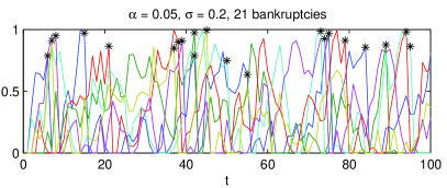
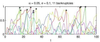
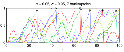
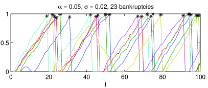
As an example, Figure 1 shows six trajectories of the stochastic process defined in Eq. (5) for a fixed value of trend strength $\alpha$ and decreasing value of noise level $\sigma$.

Figure 1: Example of six trajectories of the stochastic process for $\phi$ with fixed trend strength $\alpha$ and decreasing noise level $\sigma$. The number of failures first decreases but then increases. Since decreasing the noise level is equivalent to increasing the hedging level, the figure suggests that there is an optimal hedging level which minimizes the number of failures.

In the following, we will investigate the role of noise on the probability of failure by computing the pdf of $\phi$ in the limit of large $t$, which represents the probability distribution of fragility in the steady state of the process. Such pdf can be interpreted both as the firm’s individual probability of having a given value of fragility and as an histogram of fragility values of an ensemble of firms.

3.1 Dynamics of Fragility as Persistent Random Walk

Since varying the hedging level $k$ is equivalent to varying the noise level, in the following we definitely drop $k$ from Eq. (5) and we study the process

$$\phi(t+1)=\phi(t)+\sigma\xi(t)+\alpha\mathrm{sign}(\Delta\phi(t))$$ (5)

Assuming that the boundary conditions are not effective during two consecutive time steps, we can derive from (5) the expression of $\phi(t+2)$ in terms of $\phi(t)$.

$$\phi(t+2)=\phi(t)+\sigma(\xi(t+1)+\xi(t))+\alpha\left[\mathrm{sign}(\Delta\phi(t))+\mathrm{sign}(\sigma\xi(t)+\alpha\mathrm{sign}(\Delta\phi(t)))\right].$$ (6)

Obviously, the last term in the square parentheses can only take the values $-2,0$ or $2$, depending on the $\mathrm{sign}$ of $\Delta\phi(t)$ and the probability

$$\mathrm{Pr}(\mathrm{sign}(\sigma\xi(t)+\alpha\mathrm{sign}(\Delta\phi(t)))=\mathrm{sign}(\Delta\phi(t))).$$

This probability is

$$\mathrm{Pr}(\sigma\xi<\alpha)=\int_{-\infty}^{\alpha}f_{\sigma\xi}(x)dx=\int_{-\infty}^{\frac{\alpha}{\sigma}}f_{\xi}(x)dx$$

due to the symmetry of $f_{\xi}$. We define $q(\alpha,\sigma):=\mathrm{Pr}(\sigma\xi<\alpha)$ as the probability to keep the trend. Denoting with $F_{\xi}(x)$ the cumulative distribution function (cdf) of $\xi$ then it holds $q(\alpha,\sigma)=F_{\xi}(\frac{\alpha}{\sigma})$. We can then reformulate the process (5) as

$$\phi(t+1)=\phi(t)+\sigma\xi(t)+\alpha\mathrm{tr}(t)$$ (7)

where $\phi(t+1)$ is set to zero if it falls out of the interval $[0,\theta]$. The function ’$\mathrm{tr}$’ is the discrete stochastic process

$$\mathrm{tr}(t+1)=\eta\,\mathrm{tr}(t)\qquad\textrm{ with }\eta=\left\{\begin{array}[]{cl}1&\textrm{with probability $q$}\\ -1&\textrm{with probability $1-q$}\end{array}\right.$$ (8)

with possible initial values $\mathrm{tr}(0)=\{1,-1\}$ both with probability $\frac{1}{2}$. Notice that $\mathrm{tr}$ is not affected when $\phi$ hits any of the two thresholds. This implies that typically new firms are created with positive trend. This hypothesis simplifies the analysis but does not affect the result as discussed in Section 5.

There are two important differences between the $\mathrm{sign}$-process (5) and the trend-process (7). The first regards the behavior at the boundaries. Suppose both processes get to 0 at time $t-1$ coming from a positive value at time $t-2$ and remain at 0 at time $t$ (because, for instance, in the $\mathrm{sign}$-process $\xi(t-1)$ and $\xi(t)$ were negative and in the $\mathrm{tr}$-process $\eta(t-1)$ and $\eta(t)$ were $1$). In this case, the term $\mathrm{sign}(\Delta\phi(t))$ in Eq. (5) is zero and therefore the $\mathrm{sign}$-process will switch to a positive value at time $t+1$ with probability $\frac{1}{2}$. In contrast, the corresponding term $\mathrm{tr}(t)$ in Eq. (7) can never be zero (by definition its range is $\{-1,+1\}$ and the $\mathrm{tr}$-process will switch to a positive value at time $t+1$ with probability $1-q$. This means that when the noise $\sigma$ is small and therefore $q$ is close to $1$, the $\mathrm{tr}$-process tends to stay longer at 0, compared to the $\mathrm{sign}$-process. The $\mathrm{tr}$-process can be easily modified to better approximate the $\mathrm{sign}$-process by redefining what happens at zero. We discuss possibile modifications and their implications in Section 5.

The second difference between the two processes concerns the dependencies of the draws of the random variables. Eq. (5) implies that $\mathrm{sign}(\Delta\phi(t))=\mathrm{sign}[\xi(t-1)+\alpha\mathrm{sign}(\Delta(\phi(t-1)))]$ and therefore $\xi(t-1)$ affects directly $\phi(t)$ and indirectly also $\phi(t+1)$ through the term $\mathrm{sign}(\Delta\phi(t))$. In contrast, in the $\mathrm{tr}$-process the term $\mathrm{tr}(t)$ evolves independently of the draws of the random variable $\xi$

We now compare the $\mathrm{tr}$-process with a process called persistent random walk (PRW) in the physics literature. PRW is a variant of the classic random walk in which the walker has a probability $q$ to keep the direction and $1-q$ to switch direction. If we neglect the noise term $\sigma\xi(t)$ in (7) and start with $\phi(0)=0$, then $\phi$ evolves like a PRW on $\mathbb{Z}$. The PRW obeys the telegrapher’s equation in the continuous limit [3, 15, 19]. An important property of the PRW is that it deviates, in a transient phase, from the linear scaling of the variance of the displacement with time, $<x^{2}>\sim t$ that is characteristic of the RW. Indeed, starting with all probability mass in zero, the variance first increases quadratically, $<x^{2}>\sim t^{2}$, due to waves that start towards $-\infty$ and $+\infty$ (ballistic scaling). After a continuous transition, the variance grows linearly as in the usual RW (diffusive scaling) and in the limit of large $t$, it evolves as $\frac{q}{1-q}t$. Therefore, if $q$ is close to $1$, the variance grows still linearly for large $t$, although with a high diffusion coefficient $\frac{q}{1-q}$. Compared to a pure persistent random walk, our process includes, additionally, a continuous additive noise, a sort of reflecting lower bound at zero, an absorbing bound $\theta$ (which leads to a rebirth of firms with zero fragility), and the fact that the probability $q$ of keeping the trend depends monotonously on $\frac{\alpha}{\sigma}$.

3.2 Dynamics on the probability density function of $\phi$

In order to estimate the probability that the fragility $\phi$ hits the treshold $\theta$, we want to know how its pdf evolves in time, and in particular to estimate its stable pdf if this exists.

However, it is important to notice that, at any time step $t$, the state of the process (7) is determined both by the value of $\phi(t)$ and by the value of the trend $\mathrm{tr}(t)$ which evolves as the simple two-state process (8).

In order to study the evolution of the pdf of $\phi$ one has to study the evolution of the pdf of the whole process (7-8)

Since the trend process takes only two values, we can divide the pdf of $\phi(t)$ into two parts, corresponding to negative trend ($\mathrm{tr}(t)=-1$) and positive trend ($\mathrm{tr}(t)=+1$). We define the two functions as $f_{\phi(t)}^{-}:[0,\theta]\rightarrow\mathbb{R}_{\geq 0}$ and $f_{\phi(t)}^{+}:[0,\theta]\rightarrow\mathbb{R}_{\geq 0}$.

The pdf of the whole process is determined by the pair of functions $(f_{\phi(t)}^{-},f_{\phi(t)}^{+})$ under the condition that $\int_{0}^{\theta}f_{\phi(t)}^{-}(\phi^{\prime})+f_{\phi(t)}^{+}(\phi^{\prime})d\phi^{\prime}=1$.

From this pair of functions we can derive the pdf of $phi$ as $f_{\phi(t)}=f_{\phi(t)}^{-}+f_{\phi(t)}^{+}$. In other words, $\int_{\phi^{\prime}}^{\phi^{\prime}+d\phi^{\prime}}f_{\phi(t)}^{-}(\phi^{\prime})d\phi^{\prime}$ represents the probability to have fragility in $[\phi,\phi+d\phi]$ and at the same time a downward trend, $\mathrm{tr}(t)=-1$. Analogous relation holds for the positive trend.

It is also possible to derive the pdf of $\mathrm{tr}$ as $f_{\mathrm{tr}(t)}=(\int f_{\phi(t)}^{-},\int f_{\phi(t)}^{+})$, which is a pair of scalar values specifying the probability of having negative and positive trend and which is therefore not really a pdf but a probability mass function defined on $\{-1,+1\}$.

We also define $\delta_{\alpha}$ to be the Dirac $\delta$-distribution with mass shifted by $\alpha$ (also known as $\delta(\cdot-\alpha)$), ’$\ast$’ to be the convolution operator for functions (defined for two functions $h_{1},h_{2}:\mathbb{R}\to\mathbb{R}$ as $(h_{1}\ast h_{2})(\varphi)=\int h_{1}(y)h_{2}(\varphi-y)dx$), $f_{\sigma\xi}$ to be the pdf of the noise).

Proposition 1.

Let the pdf of $\phi(t)$ be $(f_{\phi(t)}^{-},f_{\phi(t)}^{+})$. If the stochastic evolution of $\phi$ evolves as defined in Eq. (7), then the pdf of $\phi(t+1)$ is $(f_{\phi(t+1)}^{-},f_{\phi(t+1)}^{+})$ with

$$f_{\phi(t+1)}^{-} =g_{t}^{-}\mathbb{\bf 1}_{[0,\theta]}+(b^{-}(t)+z^{-}(t))\delta_{0}$$

$$f_{\phi(t+1)}^{+} =g_{t}^{+}\mathbb{\bf 1}_{[0,\theta]}+(b^{+}(t)+z^{+}(t))\delta_{0}.$$ (9)

The functions $g_{t}^{-},g_{t}^{+}$ are defined as

$$g_{t}^{-}=(qf_{\phi(t)}^{-}\ast\delta_{-\alpha}+(1-q)f_{\phi(t)}^{+}\ast\delta_{\alpha})\ast f_{\sigma\xi}$$

$$g_{t}^{+}=((1-q)f_{\phi(t)}^{-}\ast\delta_{-\alpha}+qf_{\phi(t)}^{+}\ast\delta_{\alpha})\ast f_{\sigma\xi}$$ (10)

and $b^{-}(t)=\int_{\theta}^{+\infty}g_{t}^{-},\ b^{+}(t)=\int_{\theta}^{+\infty}g_{t}^{+}$ are the probabilities to go above $\theta$ for $\phi(t)$ with negative or, respectively, positive trend, and $z^{-}(t)=\int_{-\infty}^{0}g_{t}^{-},\quad z^{+}(t)=\int_{-\infty}^{0}g_{t}^{+}$ are the probabilities to go below zero for $\phi(t)$ with negative or, respectively, positive trend.

The successive steps in the computation of $g_{t}^{-}$ and $g_{t}^{+}$ are illustrated in Figure 2 (steps 2 to 4), while the computation of $(f_{\phi(t+1)}^{-},f_{\phi(t+1)}^{+})$ is illustrated in step 5.

Proof.

First, we look at (9). Notice that the convolution operation is commutative and distributive with respect to the operation of addition. Thus, the order of the computation does not matter.

Adding the noise term $+\sigma\xi(t)$ to $\phi(t)$ in Eq. (7), corresponds to the convolution of the pdf of $\phi(t)$ with the pdf of the noise $f_{\sigma\xi}$.

The term $\alpha\mathrm{tr}(t)$ in the same equation, implies that the part of the pdf representing the upward trend is shifted upwards by $\alpha$ and that the part representing the downward trend is shifted downwards by $\alpha$. This is because shifting a function along the $x$-axis is represented by convolution with a shifted delta-function.

If the process is on a downward trend, it will keep that trend with probability $q$ and switch with probability $(1-q)\,$. The vice-versa holds for the upward trend. Thus, a $q$-fraction of $f_{\phi(t)}^{-}$ will remain in $f_{\phi(t+1)}^{-}$, while a $(1-q)$-fraction of $f_{\phi(t)}^{+}$ will join $f_{\phi(t+1)}^{-}$. The vice-versa holds for $f^{+}$.

Finally, Eq. (10) ensures that all probability mass which overlaps the interval $[0,\theta]$ is distributed back to $[0,\theta]$. The overlapping probability mass is determined by $b^{-}(t),b^{+}(t),z^{-}(t),z^{+}(t)$ and according to the boundary conditions, it is put in a $\delta$-peek at zero, while the trend information gets conserved. ∎

Notice that other definitions for rebirth after failure can easily be modeled by changing $\delta_{0}$ in Eq. (9) to any other pdf (for example to the pdf of the uniform distribution if firms should be reborn with random and equally distributed fragility). Further on, also other rules for changes of the trend can be modeled by replacing $(b^{-}(t)+z^{-}(t))$ and $(b^{+}(t)+z^{+}(t))$ by other combinations.

To better approximate the $\mathrm{sign}$-process, one should replace $z^{-}(t)$ and $z^{+}(t)$ by $\frac{1}{2}(z^{-}(t)+z^{+}(t))$. This models the fact that a firm with fragility zero for two time steps has a zero trend, and switches with equal probability to the upward or downward trend, regardless of the former trend.

Figure 2: Shifting, trend switching, shock addition and redistribution of overlapping mass for given $f_{\phi(t)}=f^{-}_{\phi(t)}+f^{+}_{\phi(t)}$. Parameters used: $\theta=1$, $\alpha=\sigma=0.15$, the noise pdf $f_{\sigma\xi}$ is gaussian. This choice implies $q\approx 0.8413$. In step 5 $c^{-}=(b^{-}(t)+z^{-}(t))\ ,c^{+}=(b^{+}(t)+z^{+}(t))$.

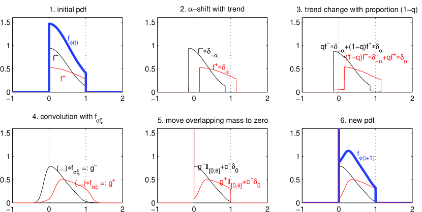
Given an initial pdf $(f^{-}_{\phi(0)},f^{+}_{\phi(0)})$, Proposition 1 defines a time-discrete evolution of the probability density function of the firm’s fragility.

In the following of this section, we will use the dynamics as defined in (9).

Proposition 2.

Consider the process defined in Eq. (7), where $\xi$ is a normally distributed random variable with mean zero, variance one and pdf $f_{\xi}$, with noise level $\sigma>0$, trend strength $\alpha\geq 0$, failing threshold $\theta$.

If $q(\alpha,\sigma)=\mathrm{Pr}(\sigma\xi<\alpha)<1$, then there exists a unique stable pdf $(f^{-}_{\ast},f^{+}_{\ast})$.

Furthermore, any initial pdf $(f^{-}_{\phi(0)},f^{+}_{\phi(0)})$ converges, under the evolution defined in Proposition 1, to $(f^{-}_{\ast},f^{+}_{\ast})$ geometrically fast, with $\int f^{-}_{\ast}=\int f^{+}_{\ast}=\frac{1}{2}$.

Proof.

We want to apply a theorem known as Birkhoff-Jentzsch Theorem [8, Page 224, Theorem 3]. It is an extension of the famous Perron-Frobenius Theorem for nonnegative matrices to infinite-dimensional vector spaces.

It is easy to see that, for any bounded pdf $(f^{-}_{\phi(t)},f^{+}_{\phi(t)})$ the two parts of the pdf $(f^{-}_{\phi(t+1)},f^{+}_{\phi(t+1)})$ are continuous on $]0,\theta]$, have a $\delta$-peak at zero and full support $[0,\theta]$. So, after one iteration the dynamics (9) remain in the space of pairs of bounded continuous functions with a $\delta$-peaks at zero.

Let us define the operator $P$ on the vector space of these functions such that it transforms $(f^{-}_{\phi(t)},f^{+}_{\phi(t)})$ into $(f^{-}_{\phi(t+1)},f^{+}_{\phi(t+1)})$. This operator fulfills the conditions of the Birkoff-Jentsch Theorem: it is in fact a uniformly positively bounded linear operator.

It is bounded because, trivially, the integral of the pdf is always one. The linearity is also easily checked since all entities in the definition of the dynamics Eqs. (9-10) are linear.

Now we show that it is also uniformly positive (as defined in [8, Page 219]). In our case an eigenvalue of $P$ must be $\lambda=1$. As lower bound for $(f^{-}_{\phi(t+1)},f^{+}_{\phi(t+1)})$ we take $(e,e)$ with $e=(1-q)c_{1}(\mathbb{\bf 1}_{[0,\theta]}+\delta_{0})$ with $c_{1}=f_{\sigma\xi}(\theta+\alpha)$. This is obviously the lowest value $(f^{-}_{\phi(t+1)},f^{+}_{\phi(t+1)})$ can take after one iteration because of convolution with $f_{\sigma\xi}$. (Take e.g. $(f^{-}_{\phi(t)},f^{+}_{\phi(t)})=(0,\delta_{\theta})$ as a ’worst case’.) Further on, an upper bound exists $c_{2}(\mathbb{\bf 1}_{[0,\theta]}+\delta_{0})$ with $c_{2}=f_{\sigma\xi}(0)$. Thus, there exists the desired strech parameter $K=c_{2}$ for the Birkoff-Jentsch Theorem.

The Birkoff-Jentsch Theorem now states that there is a unique $(f^{-}_{\ast},f^{+}_{\ast})$ and that for any inital pdf convergence to $(f^{-}_{\ast},f^{+}_{\ast})$ happens by iteration of the operator $P$ geometrically fast.

The equations $\int f^{-}_{\ast}=\int f^{+}_{\ast}=\frac{1}{2}$ are obvious, because any other distribution of mass in the parts of the pdf would not stay constant because of the equal exchange of $(1-q)$ fractions in each step. ∎

This is probably not the most general form of the theorem. Other forms of $f_{\sigma\xi}$ than normal (even with bounded support) also often lead to stabilization. But a proof is not that straight forward.

If we exchange the terms $z^{-}(t)$ and $z^{+}(t)$ by $\frac{1}{2}(z^{-}(t)+z^{+}(t))$ to better approximate the $\mathrm{sign}$-process, then fractions of mass in the parts of the still existing unique stable pdf will not be equal anymore.

From this section we conclude that there is a unique attractive stable distribution for the probability density of fragility in the $\mathrm{tr}$ process of Eq. 7. Moreover, the probability to fail at time $t$

$$b(t)=b^{-}(t)+b^{+}(t)$$ (11)

converges to fixed value which we define as the limit failure probability.

$$b^{\ast}=\lim_{t\to\infty}b(t).$$ (12)

4 Numerical results

Unfortunately, the unique stable pdf $(f^{+}_{\ast},f^{-}_{\ast})$ seems not to have a closed form, or at least not an easy one. Therefore, we compute it numerically. We set $\theta=1$ (without loss of generality) and $f_{\xi}$ to be Gaussian (with mean zero and variance one) and we explore the $(\alpha,\sigma)$-parameter space. Each pair of values $(\alpha,\sigma)$ corresponds to a value of $q$ which lies in the interval $[0.5,1]$. Notice that, assuming a different pdf for the noise would imply different values of $q$ (cf. Section 5).

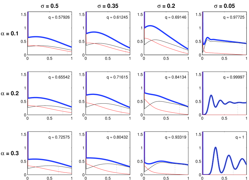
Figure 3 shows the first time steps of the pdf evolution for different $(\alpha,\sigma)$ values. Here the initial value of fragility is zero and the initial value of the trend is $\pm 1$ with equal probability. Therefore, the initial pdf is $(f^{+}_{\phi(0)},f^{-}_{\phi(0)})=\frac{1}{2}(\delta_{0},\delta_{0})$.

$\alpha=0.1,\sigma=0.3,q\approx 0.6306$

$\alpha=0.2,\sigma=0.15,q\approx 0.9088$

$\alpha=0.3,\sigma=0.1,q\approx 0.9987$

Figure 3: The first four time steps with initial pdf $f_{\phi(0)}=f^{+}_{\phi(0)}+f^{-}_{\phi(0)}=\frac{1}{2}\delta_{0}+\frac{1}{2}\delta_{0}$ and different parameters, $f_{\xi}$ is Gaussian, the $q$-values are computed from $\alpha$ and $\sigma$.

The parameter choice in the first row of plots in Figure 3 corresponds to a relatively low trend strength $\alpha$ compared to the noise level $\sigma$ and thus to a value of $q$ only slightly above its minimum $0.5$. The random term $\sigma\xi$ plays the major role in the process and in this regime the persistent random walk behaves similar to the usual random walk. This leads to a fast convergence of the pdf: after only four time steps (last plot in the row), the pdf is already close the stable pdf (cf. Figure 4). Notice that there is a significant delta peak at 0 (going beyond limit of the ordinate axis in the plot) which collects the probability to go below 0 and the probability to go above 1.

In the second row of plots in Figure 3, the values of $(\alpha,\sigma)$ correspond to values of $q$ closer to one. This implies that most of the mass of the probability density function corresponding to the downward trend ($f^{-}$) stays close to zero. On the other hand, the mass in $f^{+}$ moves with a wave towards the failure threshold (which is at 1, since the abscissa represents $\phi$ and $\theta=1$). The wave smoothes out due to the repeated convolution with $f_{\sigma\xi}$. Finally, in the third row of plots in Figure 3 $q$ is very close to one. In this case the wave towards the failure threshold repeats several times until it smoothes out. Notice that in the limit $\sigma\to 0$, and thus $q\to 1$ (not shown in the figure), the pdf of $\phi$ will not converge. There will be a delta peak which moves constantly upwards (modulo the redistribution of its mass in zero).

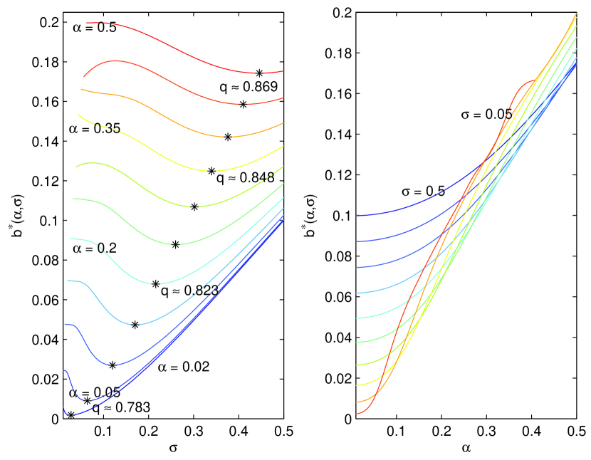
Figure 4 shows instead the stable pdfs for some specific values of $\alpha$ and $\sigma$. The pdf’s were computed by iteration of Eq. (9) with initial uniform distribution on $[0,\theta]$ and discretization of the interval $[0,1]$ in steps of $0.01$. We proceeded until the norm of the difference in one time step was smaller than an accuracy level of $10^{-6}$. There were no hints that a finer discretization would improve the result.

Figure 4: Stable pdfs for selected trend strength $\alpha$ and noise level $\sigma$ values.

The figure shows that the stable pdf is approximatively linearly decreasing for high values of fragility (except for the wavy pdf’s obtained with high $\alpha$ and low $\sigma$). The slope of the linear decrease is non-monotonously controlled by $\sigma$ and $\alpha$. It is easy to explain the slope in some cases, although this is not the case in general. When $q$ is close to 1, it is very unlikely that a trajectory of the process switches direction. A trajectories with positive trend moves steadily along the whole range of values $[0,1]$, repetitively hits the threshold 1 and gets reset to 0. In contrast a trajectory with negative trend reaches 0 and stays there. As a result, $f^{+}$ tends to a uniform distribution in $[0,1]$ and $f^{-}$ tends to a delta peak in 0. On the other hand, $q$ close to $0.5$ is implied by $\sigma$ much larger than $\alpha$. In this regime, $\phi$ diffuses very fast which leads again to a rather flat distribution for both $f^{-}$ and $f^{+}$. In contrast, for intermediate values of $q$ (for instance $\alpha=0.1,\sigma=0.2$), the profile has a pronounced negative slope for high $\phi$.

In the regime of high $\alpha$ and $\sigma$ close to 0, the trajectory evolves by almost discrete jumps of magnitude close to $\alpha$. This results in a wavy stable pdf with peaks at multiples of $\alpha$. But the wavy pattern oscillates around a line with flat slope, which is consistent with what found in the case of high $q$ and $sigma$ not too close to 0.

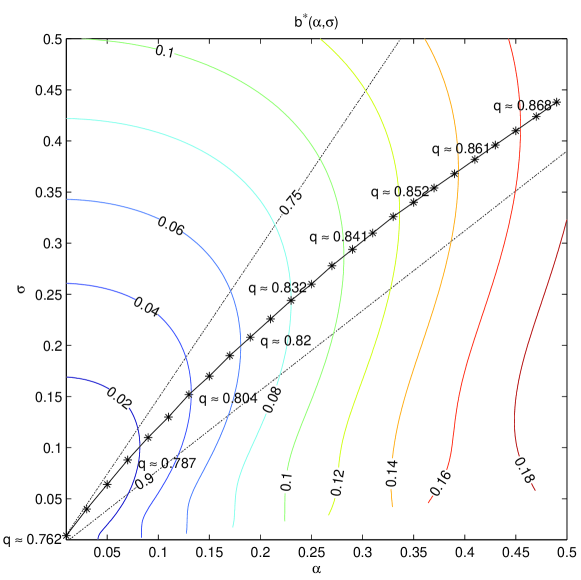
We are most interested in the limit failure probability which is our proxy for the systemic risk. It depends on trend strength $\alpha$ and noise level $\sigma$. So, we computed $b^{\ast}=b^{\ast}(\alpha,\sigma)$ for the parameter set $\alpha,\sigma\in]0,0.5]$.

Figure 6 shows that for fixed trend strength $\alpha$ there is an intermediate optimal $\sigma$ which leads to minimal systemic risk. In contrast, for a fixed noise level $\sigma$ there is no intermediate minimum when varying the trend strength $\alpha$. Raising the trend strength always increases the systemic risk. The lines for high $\sigma$ and low $\sigma$ intersect. This resembles the existence of the intermediate optimum for fixed $\alpha$.

Figure 5: The limit failure probability with respect to trend strength $\alpha$ and standard deviation of shocks $\sigma$. (Noncomplete lines are due to extremely long convergence times.)

The left plot in Figure 6 shows also values of the probability to keep the trend $q$ at the intermediate minima of the limit failure probability with respect to $\sigma$, given a fixed trend strength $\alpha$. It turns out that the optimal noise level lies at a value of $q$ roughly between $0.75$ and $0.9$. The value of $q$ corresponding to the local minimum decreases slowly with $\alpha$. This is better visible in Figure 6 where we take a bird eye’s view on the $(\alpha,\sigma)$-plane, where the level lines of equal $q$ appear as rays from the origin. The ordinate represents $q=0.5$, the abscissa $q=1$.

Figure 6: Contour plot for the limit failure probability $s(\alpha,\sigma)$ and contour lines for $q(\alpha,\sigma)=0.8,0.9$. The solid black line denotes the optimal value of $\sigma$ regarding a fixed $\alpha$.

5 Robustness of results

We checked other pdf’s for the noise besides the Gaussian and in most cases we also observe convergence to a unique stable pdf. Notice that convergence is not assured in general by Proposition 1. We observed quantitative changes in the results but not qualitative ones in the sense that there always exists an optimal noise level for a fixed trend strength.

In our model, firms fail when their fragility hits a threshold and are recreated with an initial value of fragility zero and an initial trend proportional to the number of failing firms with that trend (so mostly with upward trend). This is a strong assumption and therefore we checked three other scenarios, in particular to test whether the phenomena of an intermediate optimal noise level is robust against these modifications.

• If a new born firm is assigned a positive or negative trend with equal probability (instead of proportional to the number of failing firms of that trend) then the probability to have a positive trend $\int f^{+}_{\phi(t)}$ converges to a fixed number below $\frac{1}{2}$ which depends on $q$. In the extreme case, $q=1$ it goes to zero. That would implies that the probability to fail will also go to zero in the limit. We saw that for a fixed trend strength there is a critical noise level that implies such high $q$ that the systemic risk drops to zero when the noise level gets below. Nevertheless, for low trend strength values ($\alpha$ below about 0.12) an intermediate optimal noise level still exists until further decreasing the noise level causes the sudden drop due to the extinction of the upward trend. One may criticize this variation of the model because it does not converge to equal proportions of positive and negative trend. But stable equal probabilities for upward and downward trend seems quite reasonable because judgement of fitness is always done comparatively in an economy. If economy divides firms in good and bad ones this should not lead to a possible die out of one class.

• Another suggestion against our original model could be that firms are not born with zero fragility but i.e. random and uniformly distributed in the fragility interval. This obviously changes the limit pdf, but at least in this example the qualitative behavior with the existence of an optimal number of hedging partners for given rend strength remains the same.

• Another idea is to renormalize the probability mass after a failure. We do this as follows: we do not redistribute the probability mass after a failure to zero but just rescale $f^{+}$ proportional to its actual shape such that it has the same total amount as before. The same with $f^{-}$. On the level of individual firms this means that new firms are born with fragilities drawn randomly from the actual distribution of fragilities with that trend. That means if the distribution of fragilities is double peaked new firms are most likely to appear with fragilities around that two peaks. This dynamics imply that a given peak structure gets amplified by the evolution of new firms. In fact this dynamic fragility distribution for new firms leads to an amplification of mass in high fragility intervals. That means that with high probability new firms are born with high fragility (which seems reasoable). In the limit these regimes are characterized by virtually all firms with positve trend failing each year. That means that decreasing the noise level (which increases $q$) is even more dangerous. Nevertheless, there still exists an intermediate optimal noise level for a given trend strength to minimize the systemic risk.

6 Conclusions

We have presented a simple model for the stochastic evolution of the fragility of units in a network. The model applies in particular to networks of firms connected via financial relationships. The basic ingredients of the model consist in a mechanism of risk sharing that leads to decrease the fluctuation of the fragility and in a mechanism of reinforcing feedback on the fragility from the trend in the immediate past of the fragility of the firm itself and its neighbors. Under this assumptions, the number of bankruptcies in the system is minimized for an intermediate density of links in the network e.g. for an intermediate number of hedging partners. The result is of interest from the point of view of policy design for the control of systemic risk.

The effect depends strongly on a dynamics divisions of firms into two classes: the good evolving (with decreasing fragility) and the bad evolving firms (with increasing fragility). One might question that this hard cut between the two classes exists. But we argue that actually, slight differences in performance are exacty what investors like hedge funds search for when they try to profit from investments indepently of the economic trend. So, even very slight differences may matter a lot for reinforcing trends. Further on, these kind of investment strategies have become more popular.

With respect to the original model, the analysis presented here neglects the process of cascades of failures and therefore underestimates the number of joint failures. However, its advantage is that the evolution of the probability distribution of failures can be expressed analitically and that the stable distribution (which we prove to exist and be unique) can be computed numerically.

The impact of heterogeneity in the topology of the network is not studied at this stage. Furthermore, the hedging network is not dynamic. This implies for instance that firms do not have the possibility to interrupt hedging relations with partner who do not perform well. This assumption is certainly not very realistic on a time scale of years. However, it is also true that many partnership or insurance contracts cannot be modified in a very short time. Furthermore, in future work the impact of heterogeneous trend strength, noise level and failing threshold should be studied.

Acknowledgements

This work is part of a project within the COST Action P10 “Physics of Risk”. We appreciate financial support from the Swiss National Science Foundation under the contract number C05.0148. We thank Ulrich Krause (Bremen) for pointing us to the Birkhoff-Jentzsch Theorem. We also thank Mauro Napoletano for suggestions and helpful discussions.

References

- [1] Agata Aleksiejuk, Janusz A. Holyst, and Gueorgi Kossinets. Self-organized criticality in a model of collective bank bankruptcies. Int. Journal of Modern Physics C, 13:333, 2001.
- [2] Franklin Allen and Douglas Gale. Financial contagion. Journal of Political Economy, 108(1):1–33, February 2001.
- [3] Mariela Araujo, Shlomo Havlin, George H. Weiss, and H. Eugene Stanley. Diffusion of walkers with persistent velocities. Physical Review A, 43(10):5207–5213, 1991.
- [4] Stefano Battiston, Domenico Delli Gatti, Mauro Gallegati, B. C. N. Greenwald, and J. E. Stiglitz. Credit chains and bankruptcies avalanches in production networks. Journal of Economic Dynamics and Control, 31(6):2061–2084, 2007.
- [5] Stefano Battiston, Domenico Delli Gatti, Mauro Gallegati, Bruce C. N. Greenwald, and Joseph E. Stiglitz. Trade credit networks and systemic risk. Submitted, 2007.
- [6] Stefano Battiston, Kersten Peters, Dirk Helbing, and Frank Schweitzer. Cascades on networks. Submitted, 2007.
- [7] Roger L. Berger. A Necessary and Sufficient Condition for Reaching Consensus Using DeGroot’s Method. Journal of the American Statistical Association, 76:415–418, 1981.
- [8] G. Birkhoff. Extensions of Jentzsch’s Theorem. Transactions of the American Mathematical Society, 85(1):219–227, 1957.
- [9] F. Boissay. Credit chains and the propagation of financial distress. Working Paper 573, European Central Bank, 2006.
- [10] Markus K. Brunnermeier and Lasse Heje Pedersen. Predatory Trading. The Journal of Finance, 60(4):1825–1862, 2005.
- [11] Morris H. DeGroot. Reaching a Consensus. Journal of the American Statistical Association, 69(345):118–121, 1974.
- [12] Xavier Freixas, Bruno M. Parigi, and Jean-Charles Rochet. Systemic risk, interbank relations, and liquidity provision by the central bank. Journal of Money, Credit and Banking, 32:611–638, 2000.
- [13] S. Goldstein. On Diffusion by Discontinuous Movements, and on the Telegraph Equation. The Quarterly Journal of Mechanics and Applied Mathematics, 4(2):129, 1951.
- [14] G. Iori, S. Jafarey, and F. Padilla. Systemic risk on the interbank market. Journal of Economic Behaviour and Organization, 61(4):525–542, 2006.
- [15] Jaume Masoliver, Josep M. Porrà, and George H. Weiss. Solutions of the telegrapher’s equation in the presence of traps. Physical Review A, 45(4):2222–2227, 1991.
- [16] Eugene Seneta. Markov Chains. George Allen & Unwin Ltd., 1973.
- [17] Joseph E. Stiglitz and Bruce C.N. Greenwald. Towards a New Paradigm in Monetary Economics. Cambridge Univ. Press, Cambridge, 2003.
- [18] GI Taylor. Diffusion by Continuous Movements. Proceedings of the London Mathematical Society, 2(1):196, 1922.
- [19] George H. Weiss. Some applications of persistent random walks and thetelegraper’s equation. Physica A, 311:381–410, 2002.