Self-Similar Dynamics of a Relativistically Hot Gas

Abstract

In the presence of self-gravity, we investigate the self-similar dynamics of a relativistically hot gas with or without shocks in astrophysical processes of stellar core collapse, formation of compact objects, and supernova remnants with central voids. The model system is taken to be spherically symmetric and the conservation of specific entropy along streamlines is adopted for a relativistic hot gas whose energy-momentum relation is expressed approximately by $\varepsilon=c\mathbbm{p}$ with $\varepsilon$ and $\mathbbm{p}$ being the energy and momentum of a particle and $c$ being the speed of light. In terms of equation of state, this leads to a polytropic index $\gamma=4/3$. The conventional polytropic gas of $P=\kappa\rho^{\gamma}$, where $P$ is the thermal pressure, $\rho$ is the mass density, $\gamma$ is the polytropic index, and $\kappa$ is a global constant, is included in our theoretical model framework. Two qualitatively different solution classes arise according to the values of a simple power-law scaling index $a$, each of which is analyzed separately and systematically. With explicit conditions, all sonic critical lines appear straight. We obtain new asymptotic solutions that exist only for $\gamma=4/3$. Global and asymptotic solutions in various limits as well as eigensolutions across sonic critical lines are derived analytically and numerically with or without shocks. By specific entropy conservation along streamlines, we extend the analysis of Goldreich & Weber for a distribution of variable specific entropy with time $t$ and radius $r$ and discuss consequences in the context of a homologous core collapse prior to supernovae. As an alternative rebound shock model, we construct an Einstein-de Sitter explosion with shock connections with various outer flows including a static outer part of a singular polytropic sphere (SPS). Under the joint action of thermal pressure and self-gravity, we can also construct self-similar solutions with central spherical voids with sharp density variations along their edges.

1 Introduction

Radiation pressure (e.g., Chandrasekhar 1939, 1960; Rybicki & Lightman 1979), trapped neutrino pressure deep in the stellar interior of extremely high nuclear density, relativistically degenerate materials (e.g., Chandrasekhar 1939), extremely hot interior materials of stars, and processes likely involved in gamma-ray bursts (GRBs) etc. may be approximated by an equation of state with a polytropic index of $\gamma=4/3$. Statistical physics indicates that the state for a stationary radiation field with particles of no rest mass such as photons is described by a polytropic relation with an index $\gamma=4/3$. It is proven that $\gamma=4/3$ is also a very good approximation for relativistically hot particles with negligible rest mass. Moreover for the stellar structure, Chandrasekhar (1939) noted that for an infinitesimal uniform expansion or contraction of a gas sphere, it involves precisely a polytropic process of an index $\gamma=4/3$. For a static equilibrium configuration and a presumed $P=\kappa\rho^{\gamma}$ with a globally constant $\kappa$, the virial theorem indicates that $\gamma<4/3$ situations are unstable and $\gamma=4/3$ corresponds to a transition from unstable to stable configurations as $\gamma$ increases. When $\gamma=4/3$ for a static equilibrium configuration, the equilibrium condition is referred to as the Lane-Emden equation with the total enclosed mass $M$ being independent of the system radius but dependent upon the value of $\kappa$.

On the other hand, based on the conventional polytropic equation of state $P=\kappa\rho^{\gamma}$, where $\kappa$ is a global constant and $\gamma$ varies from $1$ for an isothermal case to $5/3$ for an adiabatic process of monatomic gas, astrophysicists explored properties of hydrodynamic behaviours in diverse contexts, such as star formation, core formation in molecular clouds and supernova explosions etc. For catching the basic physics and theoretical simplicity, most works on gravitational stellar core collapses or stellar explosions were usually carried out under the spherical symmetry. Hunter (1962) considered the stability of an equilibrium system and the collapse process based on a polytropic hydrodynamics. He demonstrated how a dynamical instability during the collapse leads to a breakup of the spherically symmetric radial inflow of gas. Shu (1977) constructed the isothermal expansion-wave collapse solution (EWCS) with a weak discontinuity; and this self-similar hydrodynamic model has been further developed in the past three decades, from the isothermal case (e.g., Shu 1977; Lou & Shen 2004) to the polytropic case (e.g., Suto & Silk 1988; Yahil 1983; Lou & Wang 2006), as well as to the logotropic case (e.g., Mclaughlin & Pudritz 1997). Observationally, spectral lines of CS, H₂CO and other molecules in star forming regions show that the single peak of each molecular line splits into double peaks with the blue peak brighter than the red peak, which has been regarded as a supporting evidence to the Shu model (e.g. Zhou 1992; Walker, Narayanan & Boss 1994; Myers et al. 1996). It is generally expected that shock waves are also involved in self-similar collapse or expansion profiles (e.g., Tsai & Hsu 1995; Shu et al. 2002; Bian & Lou 2005).

Note that all above studies were carried out on either the isothermal case or the $\gamma\neq 4/3$ polytropic case. In one case, the polytropic case of $\gamma=4/3$ is treated as a limiting case (Yahil 1983). In contrast, Goldreich & Weber (1980) directly considered homologous core collapse for a conventional polytropic gas with $\gamma=4/3$ by making use of the time reversal invariance. They concluded that when the pressure decreases by a fraction of no more than about $3\%$ from a static polytrope in equilibrium, a homologous core collapse would occur in the stellar interior. On the other hand, numerical simulation of Bethe et al. (1979) indicated a fractional reduction of pressure by $26\%$ in order to initiate a core collapse for a supernova explosion. Goldreich & Weber (1980) tried to reduce this difference by introducing an inner core of a progenitor star; Yahil (1983) performed his polytropic analysis and treated their result as a limit of $\gamma\rightarrow 4/3^{+}$.

Meanwhile, specific entropy conservation along streamlines does not necessarily mean a constant specific entropy everywhere at all times. A more general distribution would be a variable specific entropy in time and radius (e.g. Cheng 1977, 1978). Fatuzzo et al. (2004) introduced a self-similar transformation to formulate a more general problem, which involves a scaling index $a$ and another index $q$. The more general equation of state appears to be $P\propto M^{q}\rho^{\gamma}$. The $q=0$ case corresponds to the conventional polytropic gas. In fact, according to this more general equation of state, the conservation of mass implies the conservation of specific entropy along streamlines. Nevertheless, Fatuzzo et al. (2004) mainly focused on the isothermal cases with nonzero inward flow speeds far away in molecular clouds (Shen & Lou 2004).

Our consideration is on a more general polytropic gas with $\gamma=4/3$ with the specific entropy conserved along streamlines. By a self-similar transformation, we can approach the resulting nonlinear ordinary differential equations (ODEs) systematically. Solution properties depend on the scaling index $a$. Given a distribution of variable specific entropy with time and radius, the result of Goldreich & Weber (1980) can be substantially extended. Meanwhile, many counterparts of previously known solutions in the isothermal and conventional polytropic cases can also be derived. In particular, several new asymptotic solutions unique to $\gamma=4/3$ are also obtained. An important and interesting result of our analysis is that under the joint action of thermal pressure force and self-gravity, a central spherical void can form and evolve in a self-similar manner; this is to be compared with the central spherical void solution of Fillmore & Goldreich (1984b) which considered a collection of collisionless particles under self-gravity in the Einstein-de Sitter expanding universe.

This paper is structured as follows. Nonlinear adiabatic hydrodynamic equations in spherical symmetry and self-similar transformation are described in Section 2 for a polytropic gas with a polytropic index $\gamma=4/3$. The extensions of the classical analysis of Goldreich & Weber (1980) are presented in Section 3 and further discussed for a homologous stellar core collapse in Section 6.1. We mainly focus on cases of $q=2/3$ for various solution properties such as the requirement on the scaling index $a$, the property of scaling invariance, global analytic solutions, the sonic singular surface, the straight sonic critical lines, eigensolutions across the sonic critical line, various asymptotic solutions, and shock jump conditions in Sections 4. We analyze various semi-complete numerical solutions with or without shocks and corresponding results in Section 5. Finally, we conclude and discuss our main results in Section 6. Three Appendices A, B and C are included at the end for technical details of derivations and analyses.

2 Basic Nonlinear Equations and Self-Similar Transformation

As a theoretical model formulation, dynamical processes outlined in introduction are governed by the basic nonlinear hydrodynamic equations under the assumption of spherical symmetry. We naturally adopt the spherical polar coordinates $(r,\ \theta,\ \phi)$ in the analysis. The mass conservation is

$$\frac{\partial M}{\partial t}+u\frac{\partial M}{\partial r}=0\quad\qquad\mbox{ and }\quad\qquad\frac{\partial M}{\partial r}=4\pi r^{2}\rho\ ,$$ (1)

where $M(r,t)$ is the enclosed mass within radius $r$ at time $t$, the mass density $\rho(r,t)$ is a function of $r$ and $t$ and $u(r,t)$ is the radial flow velocity. The above two relations in equation (1) are equivalent to the mass continuity equation

$$\frac{\partial\rho}{\partial t}+\frac{1}{r^{2}}\frac{\partial}{\partial r}(r^{2}\rho u)=0\ .$$ (2)

The gas motion is governed by the radial momentum equation

$$\frac{\partial u}{\partial t}+u\frac{\partial u}{\partial r}=-\frac{1}{\rho}\frac{\partial P}{\partial r}-\frac{GM}{r^{2}}\ ,$$ (3)

where $P(r,t)$ is the thermal gas pressure and $G=6.67\times 10^{-8}\hbox{ dyne-cm}^{2}\hbox{ g}^{-2}$ is the gravitational constant. The Poisson equation relating the mass density $\rho$ and the gravitational potential $\Phi(r,t)$ is automatically satisfied with $\partial\Phi/\partial r=GM/r^{2}$. Finally, the conservation of specific entropy $s(r,t)$ along streamlines is simply

$$\left(\frac{\partial}{\partial t}+u\frac{\partial}{\partial r}\right)\left(\frac{P}{\rho^{\gamma}}\right)=0\ ,$$ (4)

where $\gamma$ is the polytropic index. We note that $P=\kappa\rho^{\gamma}$ with a constant $\kappa$ is just a particular case satisfying equation (4). Combining the conservation laws of mass and specific entropy, the specific entropy $s(r,t)$ can be an arbitrary function $s=s(M)$ of the enclosed mass $M(r,t)$. The entropy is a statistical quantity associated with a large number of particles, it appears that in this situation, the entropy is frozen in particles along streamlines. By this consideration, we have

$$\frac{ds}{dt}=\frac{ds}{dM}\frac{dM}{dt}=0\$$ (5)

with

$$\frac{d}{dt}=\frac{\partial}{\partial t}+u\frac{\partial}{\partial r}$$ (6)

being the total time derivative along a streamline.

2.1 Self-Similar Transformation

In order to solve for self-similar solutions from these nonlinear partial differential equations, we introduce the following self-similar transformation to reduce equations $(\ref{eq01})-(\ref{eq04})$ to nonlinear ODEs, namely

$$x=At^{a}r\ ,\qquad\rho=\frac{\alpha(x)}{4\pi Gt^{2}}\ ,\qquad M=\frac{m(x)}{A^{3}Gt^{3a+2}}\ ,$$

$$u=\frac{v(x)}{At^{a+1}}\ ,\qquad P=\frac{p(x)}{4\pi GA^{2}t^{2(a+2)}}\ ,\qquad\qquad\quad$$ (7)

where $a$ is an important scaling index parameter and $A$ is a dimensional constant coefficient to make the independent variable $x$ dimensionless. Here, $\alpha(x)$, $m(x)$, $v(x)$, and $p(x)$ are functions of $x$ only and are referred to as the reduced density, enclosed mass, velocity and pressure, respectively. Now with self-similar transformation (7), equations $(\ref{eq01})-(\ref{eq04})$ take the form of

$$(ax+v)\frac{dm}{dx}=(3a+2)m\ ,$$ (8)

$$\frac{dm}{dx}=x^{2}\alpha\ ,$$ (9)

$$(ax+v)\frac{dv}{dx}+\frac{1}{\alpha}\frac{dp}{dx}=-\frac{m}{x^{2}}+(a+1)v\ ,$$ (10)

$$(ax+v)\frac{d}{dx}\log\bigg{(}\frac{p}{\alpha^{\gamma}}\bigg{)}=2(2+a-\gamma)\ ,$$ (11)

$$(ax+v)\frac{1}{\alpha}\frac{d\alpha}{dx}+\frac{dv}{dx}=2\left(1-\frac{v}{x}\right)\$$ (12)

(Fatuzzo et al. 2004; Wang & Lou 2007). Before proceeding, we note that these equations are invariant under the following time reversal transformation, namely

$$r\rightarrow r\ ,\qquad t\rightarrow-t\ ,\qquad u\rightarrow-u\ ,$$

$$\rho\rightarrow\rho\ ,\qquad M\rightarrow M\ ,\qquad P\rightarrow P\ .$$ (13)

Therefore any solution can also depict its inverse process as long as this process is reversible (e.g., not involving shocks). For example, one solution describing a collapse can be also utilized to describe an expansion process. More importantly, equation (8) implies a division of all cases into three classes by whether or not scaling parameter $a$ is greater than, equal to or less than $-2/3$; in general, $a$ is required to be negative.

This requirement of a negative $a$ is not obvious by equations (7)$-$(12). By the asymptotic solutions (36) and (48) at large $x$ derived later, it is necessary to require $a<0$ for convergent solutions at large $x$.

3 Homologous Core Collapses

We first analyze the case of $a=-2/3$ precisely which includes the classical analysis of Goldreich & Weber (1980). Their model was applied to a stellar core collapse under self-gravity prior to the core bouncing in the context of supernova explosions. By equations (8) and (9), we simply have

$$(ax+v)x^{2}\alpha=0\ .$$ (14)

The case of $\alpha=0$ everywhere at all time would be a trivial solution; for nontrivial solution, the radial flow velocity is thus given by

$$v=-ax=2x/3\ ,$$ (15)

and then equation (11) requires $\gamma-a=2$ leading to $\gamma=4/3$ precisely. Here $v(x)$ represents an expansion solution, or a core collapse solution with the time reversal invariance transformation. Meanwhile, equation (12) becomes automatically satisfied under this transformation, giving no further information or constraint. Taking the derivative of equation (10) with respect to $x$, we derive

$$\frac{1}{x^{2}}\frac{d}{dx}\left(\frac{x^{2}}{\alpha}\frac{dp}{dx}\right)=-\alpha+\frac{2}{3}\ .$$ (16)

Now these equations are not complete yet and a more general description of specific entropy distribution as a function of $x$ is allowed. In other words, we already get $P\propto\rho^{4/3}$ but do not know the proportional coefficient as a function of $(r,\ t)$ which is associated with the enclosed mass $M(r,\ t)$. In fact, this point can also been seen by directly comparing $P$ and $\rho$ in self-similar transformation (7). Physically, $\log(P/\rho^{4/3})$ is proportional to the specific entropy $s(r,t)$ in a polytropic gas. Once we know the distribution of specific entropy as a function of $x$, the self-similar polytropic flow is then determined.

The first cut is to take a constant specific entropy everywhere at all times, i.e., $P=\kappa\rho^{4/3}$ with $\kappa$ being a global constant. In fact, this is exactly what Goldreich & Weber (1980) did. For $A=(4\pi G/\kappa^{3})^{1/6}$ in self-similar transformation (7), we immediately obtain $p=\alpha^{4/3}$ and a second-order ODE for $\alpha$ from equation (16). We may write $\alpha=f^{3}$ for the convenience of comparison and the second-order nonlinear ODE for $f(x)$ with a central condition is then

$$\left\{\begin{array}[]{l}\displaystyle\frac{d^{2}f}{dx^{2}}+\frac{2}{x}\frac{df}{dx}+\frac{f^{3}}{4}=\frac{1}{6}\ ,\\ f^{\prime}(0)=0\ ,\end{array}\right.$$ (19)

where $f(0)>0$ is related to the central mass density and is an adjustable parameter up to $f_{c}$. In numerical integrations, we may encounter $f(x)=0$ at a finite $x>0$ under certain conditions. If this is the case, an outer travelling boundary of the flow system exists. It is fairly straightforward to solve equation (19) numerically by the standard Runge-Kutta scheme (e.g., Press et al. 1986).

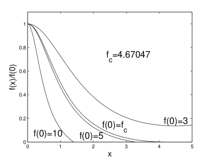
Figure 1: Profiles of $f(x)$, closely related to the reduced mass density by $\alpha(x)=f^{3}(x)$, with different values of $f(0)$ are shown for a globally constant specific entropy distribution. Here, $f(x)$ is normalized by $f(0)$ which is related to the central mass density. There exists a limiting value $f(0)=f_{c}$ such that if and only if $f(0)>f_{c}$, the solution curve $f(x)$ vanishes at a finite $x>0$. The value $f_{c}=4.67047$ is numerically determined. To show this transition, we take $f(0)=3.0,\ f_{c},\ 5.0,\ 10.0$ in turn as examples of illustration. For $f(0)<f_{c}$, the solution would have a density profile of an infinite extent and the radial flow velocity diverges for large $x$. The curves $f(x)$ give self-similar profiles of density distribution for a spherical expansion. The process of collapse can be also described by a time reversal operation.

We have just summarized essential results of Goldreich & Weber (1980) in their analysis. Through numerical exploration, we also find that there exists a limiting value for $f(0)$ denoted by $f_{c}=4.67047$ (see Figure 1). With $f(0)$ greater than this critical value $f_{c}$ at $x=0$, the solution of $f(x)$ is confined by a finite $x$ and has plausible physical properties. For $f(0)<f_{c}$, the mass density does not vanish at a finite $x>0$ and does not approach zero for large $x$ either. By comparing our adjustable parameter $f(0)$ with parameter $\lambda$ of Goldreich & Weber (1980), we readily establish the following simple conversion relation

$$\lambda f^{3}(0)=2/3\ .$$ (20)

Parameter $\lambda$ has a maximum value as noted by Goldreich & Weber (1980); their maximum value $\lambda_{m}=0.00654376$ corresponds to our $f_{c}$ well. Our $f_{c}=4.67047$ gives a $\lambda_{m}=0.00654375$. When $f(0)$ is lower than this minimum value $f_{c}$, there is no self-similar solution with vanishing density at a finite $x\neq 0$. Physically, $f_{c}$ corresponds to the minimum central density for a homologous or self-similar core collapse to be possible.

In addition to the preceding analysis, our polytropic model analysis here does not necessarily require a constant specific entropy everywhere (in time and space) and therefore substantially generalizes the work of Goldreich & Weber (1980). In fact, we can allow for a fairly arbitrary distribution of specific entropy and therefore accommodate a broad class of solutions for the density profile. A proper distribution of specific entropy can be described by

$$p=g(x)\alpha^{4/3}\$$ (21)

where $g(x)$ is a sensible but otherwise arbitrary function. In fact, the case studied by Goldreich & Weber (1980) simply corresponds to $g(x)=1$. For a more general $g(x)$, we readily derive a second-order nonlinear ODE for $f(x)$ and a central condition, namely

$$4gf^{\prime\prime}+\bigg{(}5g^{\prime}+\frac{8g}{x}\bigg{)}f^{\prime}+\frac{2}{x}fg^{\prime}+fg^{\prime\prime}+f^{3}=\frac{2}{3}\ ,$$

$$p^{\prime}(0)=0\Rightarrow g^{\prime}(0)f(0)+4g(0)f^{\prime}(0)=0\ ,$$ (22)

where prime “$\prime$” indicates a derivative with respect to $x$ and $\alpha(x)=f^{3}(x)$ is the reduced mass density. Now given a value of $f(0)$, related to the central mass density, we can solve $f(x)$ numerically to determine the self-similar mass density profile. The intersection of $f(x)$ with the $x$ axis is the moving ‘boundary’ of the flow system, denoted by $x_{b}$.

As we know the density profile, we can calculate the enclosed mass $m(x)$ and the ratio between the central and mean densities. As shown by equation (9), the enclosed mass is

$$m(x_{b})=\int_{0}^{x_{b}}x^{2}\alpha dx\ .$$ (23)

Using equation (16), one can readily get

$$m(x_{b})=2x_{b}^{3}/9-4x_{b}^{2}g(x_{b})f^{\prime}(x_{b})$$ (24)

and the dimensional enclosed mass is expressed as

$$M=\frac{m(x_{b})}{A^{3}G}=\frac{1}{A^{3}G}\left[\frac{2}{9}x_{b}^{3}-4x_{b}^{2}g(x_{b})f^{\prime}(x_{b})\right]\ .$$ (25)

The ratio between the mean and central densities is

$$\frac{\bar{\rho}}{\rho_{c}}=\frac{3}{f^{3}(0)}\left[\frac{2}{9}-\frac{4g(x_{b})f^{\prime}(x_{b})}{x_{b}}\right]\ .$$ (26)

We are now in a position to make a comparison. With $g(x)=1$, Goldreich & Weber (1980; GW) computed the above quantities; within numerical errors, the results of theirs and ours are mutually consistent. Our result of $\bar{\rho}/\rho_{c}$ varies between $0.0066$ and $0.0185$, while theirs varies between $0.0065$ and $0.0185$. The value of $m(x_{b})$, similar to $r_{b}^{3}\bar{\rho}/\rho_{c}$ in GW, increases by a factor of 1.045 when $f(0)$ increases from $f_{c}$ to a sufficiently large value, which is also equal to that of GW.

As examples of illustration, we shall prescribe specific functional forms of $g(x)$ and analyze corresponding solutions of $f(x)$ presently in Section 6.3.

4 Various Solution Properties

In this section, we mainly focus on cases with $a\neq-2/3$. In these cases, it is still possible for $\gamma=4/3$ which was not considered by Goldreich & Weber (1980) and Yahil (1983).

4.1 A Preliminary Consideration

We turn to reduced nonlinear ODEs (8)$-$(12) to start our discussion. First, a combination of equations (8) and (9) immediately gives the reduced mass as

$$m(x)=\frac{(ax+v)}{(3a+2)}x^{2}\alpha(x)\ .$$ (27)

By equation (27), no confined solution for $\alpha(x)$ by a finite value of $x>0$ exists because $\alpha=0$ at a finite $x$ directly leads to $m=0$, i.e., no enclosed mass at all within this $x$ where the mass density vanishes. As a result, no solutions can be confined by a finite $x>0$. In these cases, the $x$ range of both analytical and numerical solutions is infinite and some sensible cutoffs need to be introduced for astrophysical applications. Moreover, the enclosed mass should be always positive such that $(ax+v)/(3a+2)>0$. For $a<-2/3$, we must require $v<-ax$, while for $a>-2/3$, we should have $v>-ax$. This is a strict constraint of self-similar transformation such that no decreasing solutions of $v(x)$ exist for $a>-2/3$. In general, $a$ should be always less than $0$ because of the requirement of a real physical system. Dividing equation (11) by equation (8), we obtain

$$p=C_{0}m^{q}\alpha^{\gamma}\ ,$$ (28)

where another index parameter $q$ is defined by

$$q\equiv 2(2+a-\gamma)/(3a+2)$$ (29)

and $C_{0}$ is a constant of integration. This carries an apparent physical meaning. It is mentioned earlier that if the specific entropy is a function of the enclosed mass, the conservation of specific entropy along streamlines is automatically satisfied. The similarity transformation then gives a more specific constraint on the form of this function, which is proportional to $M^{q}$. Substituting the dimensionless quantities for dimensional ones, we explicitly obtain

$$P=C_{0}A^{3q-2}(4\pi G)^{\gamma-1}G^{q}M^{q}\rho^{\gamma}\ .$$ (30)

Here we have two constant coefficients: $A$ is introduced in the transformation and $C_{0}$ is a constant of integration. For $\gamma\neq 4/3$ and thus $q\neq 2/3$, we can adjust the value of $C_{0}$ and $A$ such that $C_{0}=1$ (see Lou & Wang 2007 for more details). In this paper, however, we focus on the case of $\gamma=4/3$ and thus $q=2/3$. The constant $A$ no longer plays an important role because the exponent index vanishes in expression (30) and thus disappears. In contrast, $C_{0}$ becomes vital in our case under consideration. On one hand, the local specific entropy is

$$s=\log\left(\frac{P}{\rho^{4/3}}\right)=\log{C_{0}}+\frac{1}{3}\log(4\pi G)+\frac{2}{3}\log(GM)\ .$$ (31)

The value of $C_{0}$ is related to the specific entropy. On the other hand, the local polytropic sound speed is

$$c_{s}=\left(\frac{\partial P}{\partial\rho}\right)_{s}^{1/2}=\bigg{(}\frac{4P}{3\rho}\bigg{)}^{1/2}=\left(\frac{4C_{0}\pi^{2/3}GM^{2/3}\rho^{1/3}}{3}\right)^{1/2}$$ (32)

which is also related to the value of $C_{0}$. The value of $C_{0}$ will affect our equations and thus solutions in a nontrivial manner.

Substituting equations (28) and (27) into equations (10) and (12), we readily obtain two coupled nonlinear ODEs

$$(ax+v)\frac{dv}{dx}+\frac{4C_{0}}{3}x^{4/3}\left(\frac{ax+v}{3a+2}\right)^{2/3}\frac{d\alpha}{dx}=\qquad\qquad$$

$$\quad-\frac{ax+v}{3a+2}\alpha+(a+1)v-\frac{2C_{0}}{3}\left(\frac{ax+v}{3a+2}\right)^{-1/3}x^{4/3}\alpha\ ,$$ (33)

$$\frac{dv}{dx}+\frac{(ax+v)}{\alpha}\frac{d\alpha}{dx}=2\left(1-\frac{v}{x}\right)\ .\qquad$$ (34)

Explicit expressions of these two equations for $dv/dx$ and $d\alpha/dx$ are contained in Appendix A. Our subsequent analysis is based on these two coupled nonlinear ODEs (33) and (34). Before a further discussion, one notes that besides the time reversal invariance, ODEs (33) and (34) are also invariant under the following scaling transformation, namely

$$x\rightarrow\eta x\ ,\quad\qquad\alpha\rightarrow\alpha\ ,\quad\qquad m\rightarrow\eta^{3}m\ ,$$

$$v\rightarrow\eta v\ ,\quad\qquad p\rightarrow\eta^{2}p\ ,$$ (35)

where $\eta$ is an arbitrary positive constant. This scale invariance only exists when $\gamma=4/3$ or $q=2/3$ and brings us considerable convenience in theoretical analysis.

4.2 Global Analytic Solutions

Previously, two kinds of analytic solutions were found, namely, the static singular polytropic sphere (SPS) solution and the Einstein-de Sitter expansion solution in the Newtonian regime (e.g., Wang & Lou 2007). We confirm that for the current special case of $\gamma=4/3$, these two solutions still exist with certain modifications and constraints. For the former, we note that no static SPS solution exists for $0>a>-2/3$ because of inequality $v>-ax>0$. For $a<-2/3$, we can set $v=0$ in the two ODEs and obtain

$$\alpha=Bx^{2/a}\ ,$$ (36)

$$C_{0}=-\frac{(3a+2)}{2(a+2)}\left(\frac{a}{3a+2}\right)^{4/3}\ ,$$ (37)

where $B>0$ is an arbitrary positive coefficient. Unlike previous polytropic models with $\gamma\neq 4/3$, parameter $C_{0}$ here is specifically determined by a chosen $a<-2/3$ in the model. It implies that the system requires a special relationship between the thermal gas pressure and the combination of $M^{2/3}\rho^{4/3}$ to keep the system in a radial force balance.

The so-called Einstein-de Sitter solution in the Newtonian approximation with a constant mass density also exists here for $\gamma=4/3$. By taking a constant density, we obtain

$$v=\frac{2}{3}x\ ,\qquad\alpha=\frac{2}{3}\Big{(}1+2\sqrt[3]{3}C_{0}\Big{)}^{-1}\ ,$$

$$m=\frac{2x^{3}}{9}\Big{(}1+2\sqrt[3]{3}C_{0}\Big{)}^{-1}\ ,$$ (38)

where $C_{0}>0$ is fairly arbitrary. This solution is independent of $a$ value as long as $a<-2/3$ and describes a homogeneous expansion in the Newtonian cosmology. In our case, the constant $\alpha$ is somewhat different from those of the cases with $q=0$ and $\gamma\neq 4/3$ (i.e., a conventional polytropic gas with a constant specific entropy everywhere). We also find that this kind of solutions exists only in two situations: one is $q=0$ and $a<-2/3$ (see equations (24) and (25) of Fatuzzo et al. (2004)), while the other is $q=2/3$ also with $a<-2/3$ obtained above.

It is easy to prove that the Einstein-de Sitter solution only exists in two cases for $q=0$ and $q=2/3$. For $\alpha$ being constant in ODEs (8)$-$(12), equation (9) gives

$$m=x^{3}\alpha/3\ ,$$ (39)

where a natural boundary condition is simply $m(0)=0$. Equation (8) then leads to $v=2x/3$ which also satisfies equation (12). It follows from ODEs (39) and (10) that

$$\alpha^{\gamma}C_{0}q(\alpha/3)^{q-1}x^{3q-1}=(2/9-\alpha/3)x\$$ (40)

with $\alpha$ being a constant. It is clear that for $q=0$, we have $\alpha=2/3$, while for $q=2/3$, we have a different constant $\alpha=2/(3+2C_{0}3^{4/3})$ as indicated by solution (38) at $\gamma=4/3$ and $a<-2/3$. For $q$ not equal to these two special values, no Einstein-de Sitter solution is possible. However for $a=-2/3$ precisely as in Section 3, equation (11) is of a $0=0$ form and equation (10) defines a particular form of $g(x)$, that is,

$$g(x)=\left(\frac{1}{9f}-\frac{f^{2}}{6}\right)x^{2}\ ,$$ (41)

where $f(x)=\alpha^{1/3}$ is also a constant. By the property of time reversal invariance, this may also describe a particular homologous collapse with $\alpha(x)$ being constant and a finite reference radius.

4.3 Singular Surface and Sonic Critical Line

When the determinant of the coefficient matrix of equations (33) and (34) vanishes (see Appendix A), i.e.,

$$(ax+v)^{2}=\frac{4C_{0}}{3}\left(\frac{ax+v}{3a+2}\right)^{2/3}x^{4/3}\alpha\ ,$$ (42)

where the right-hand side is the polytropic sound speed squared, the relevant ODEs (33) and (34) become singular and no finite first derivatives can be obtained (see Appendix A). This singularity determines a particular surface, referred to as the sonic singular surface in the three variable space of $x$, $v$ and $\alpha$. Any solution encountering this sonic singular surface would diverge except for certain special cases which call for additional requirements. One possibility is to go across the sonic critical curve with weak discontinuities (e.g., Whitworth & Summers 1985 for an isothermal gas) or to jump across the sonic singular surface with shocks (e.g., Tsai & Hsu 1985; Shu et al. 2002; Bian & Lou 2005; Yu, Lou, Bian & Wu 2006; Lou & Gao 2006; Lou & Wang 2006). Another possibility is to go across the sonic critical curve smoothly, for which the values of $\alpha$ and $v$ as well as corresponding derivatives satisfies critical conditions at the intersection point with the sonic singular surface.

4.3.1 Determination of the Sonic Critical Line

A necessary condition for the existence of first derivatives $\alpha^{\prime}(x)$ and $v^{\prime}(x)$ is to require

$$-\frac{ax+v}{3a+2}\alpha+(a+1)v-\frac{2C_{0}}{3}\left(\frac{ax+v}{3a+2}\right)^{-1/3}x^{4/3}\alpha$$

$$=2(ax+v)\left(1-\frac{v}{x}\right)\ .$$ (43)

This equation defines a unique curve on the sonic singular surface, which can be crossed by analytically smooth solutions; this curve is referred to as the sonic critical curve because it is physically related to the local sound speed $c_{s}$.

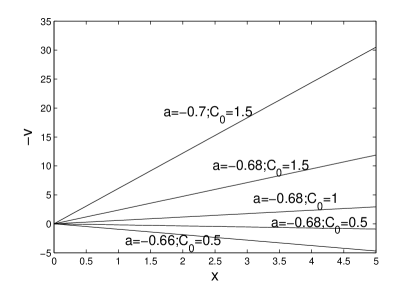
Figure 2: Behaviours of the sonic critical lines with different values of $C_{0}$ and $a$. From $(a=-0.7,\ C_{0}=1.5)$ above to $(a=-0.66,\ C_{0}=0.5)$ below in order, the corresponding values of slope $k$ are $-6.1045,\ -2.3754,\ -0.5863,\ 0.1815,\ 0.9399$, respectively. They are all rays starting from the origin in the semi-complete solution space of $-v$ versus $x$.

Reliable numerical experiments can give us valuable guidance for conceptual and analytical analysis. Through extensive numerical exploration (see Figure 2), it is shown that the sonic critical curve defined as the intersection of two surfaces given by equations (42) and (43) seems to be straight lines starting from the origin in the $-v$ versus $x$ plane and $\alpha$ remains constant along the straight sonic critical lines. Using equation (42) to eliminate $\alpha$ in equation (43), a simple derivation gives $v=kx$ with the slope $k$ being determined by

$$-\frac{3(3a+2)^{2}}{4C_{0}}\left(\frac{a+k}{3a+2}\right)^{7/3}+(a+1)k\qquad\qquad\quad$$

$$\qquad\qquad\quad-(3a+2)(a+k)/2=2(1-k)(a+k)\ .$$ (44)

Then, the corresponding value of constant $\alpha$ is given by

$$\alpha=\frac{3(3a+2)^{2}}{4C_{0}}\left(\frac{a+k}{3a+2}\right)^{4/3}\ .$$ (45)

Once $k$ is solved numerically with given values of parameter pair $a$ and $C_{0}$, the relevant sonic critical line is determined with a corresponding constant $\alpha$. As a consistent confirmation, we can also use equation (42) to eliminate $v$ and then obtain an algebraic equation for $\alpha$ independent of $x$. The same conclusion can be reached. Our extensive numerical experiments also agree with our analytical analysis as expected (see Figure 2).

For isothermal cases, the projection of the sonic singular surface coincides with that of the sonic critical line. Thus in the $-v$ versus $x$ plane, the behaviour of critical line can also show that of the singular surface. Nevertheless, in our situation the shape of the singular surface is fairly complicated and the critical curve is just a special curve embedded in it. The projection of the curve in the $-v$ versus $x$ plane cannot show the exact shape of the entire singular surface. This is very important in the discussion of shocks because a shock solution needs to jump across the sonic singular surface rather than the sonic critical curve.

4.3.2 Eigensolutions across the Sonic Critical Line

One solution seldom crosses the sonic singular surface smoothly even if it meets the sonic critical line. There are also some constraints on derivatives of proper solutions. For an arbitrary point along the sonic critical line, denoted by $x_{c}$ here, we can expand an analytic solution in terms of Taylor series expansion in the vicinity of this sonic critical point. Because the nonlinear ODEs is of second-order, only the first two terms of the series expansion need to be considered. We write

$$x=x_{c}+\delta\ ,\qquad v=v_{c}+\delta v_{1}\ ,\qquad\alpha=\alpha_{c}+\delta\alpha_{1}\ ,$$ (46)

where $v_{c}$ and $\alpha_{c}$ are the values at the sonic critical point with $v_{1}$ and $\alpha_{1}$ being the corresponding first derivatives of $v$ and $\alpha$ at $x_{c}$, and $\delta$ is a small displacement away from the critical point $x_{c}$. Substituting expression (46) into coupled nonlinear ODEs (33) and (34) and keeping in mind $v_{c}=kx_{c}$ and expression (45) for $\alpha_{c}$, it is fairly straightforward to derive a quadratic equation for $v_{1}$, namely

$$-\frac{7}{3}v_{1}^{2}+\left(7+5a-\frac{4}{3}k\right)v_{1}-\frac{10}{3}k^{2}+ak+6k\qquad\quad$$

$$-\frac{3}{2}a^{2}-6a-6-\frac{\alpha_{c}\left[a+2(1-k)\right]}{(3a+2)}=0\ .$$ (47)

Once the two first derivatives are determined, higher-order derivatives can be calculated systematically according to nonlinear ODEs (33) and (34). The two eigenvalues of the velocity first derivative $v_{1}\equiv dv/dx$ are independent of the position of critical point $x_{c}$, as shown in equation (47), which is fundamentally related to the scaling invariance equation (35) discussed earlier. Generally speaking, quadratic equation (47) has two real roots or a pair of complex conjugate roots. Because of the implicit expression of $k$, we are not able to give an analytical analysis to decide the existence of real roots. However in our numerical exploration, all roots are real; that is, for a given values of $a$ and $C_{0}$ in our experiments, the eigenvalue problem has two real roots so far.

Numerical tests also show qualitatively different behaviours corresponding to the two eigensolutions across the sonic critical curve. To examine global properties of these two, one can integrate from the critical point both outwards and inwards, with initial values given by the series expansion solutions in the vicinity of the critical point. We call the eigensolution which diverges as $x$ approaching infinity as Type I while the other that converges at large $x$ is referred to as Type II. The classification of Types I and II solutions is merely for the convenience of discussion.

4.4 Various Kinds of Asymptotic Solutions

In addition to the two global analytic solutions presented above, we also derive various asymptotic solutions either near the centre (i.e., $x\rightarrow 0^{+}$) or at infinity (i.e., $x\rightarrow+\infty$). Because $a>-2/3$ strongly limits solution behaviours such that $v$ remains always positive and diverges as $x$ approaches infinity, we focus on cases of $a<-2/3$. Previously known asymptotic solutions will guide us to search for their counterparts in the case of $\gamma=4/3$ and other possible new solutions should they exist.

By assuming $|v(x)|$ and $\alpha(x)$ to be nonincreasing functions for large $x$, the first typical asymptotic solutions are

$$\alpha=Hx^{2/a},\quad v=Lx^{(a+1)/a}+Kx^{(2+a)/a}\ ,\quad(x\gg 1)$$ (48)

where $H>0$ and $L$ are two constants of integration, $\gamma=4/3$, and $K$ is determined by

$$K=-\frac{aH}{(3a+2)}-2C_{0}H\left(\frac{a}{3a+2}\right)^{-1/3}\frac{(a+2)}{(3a+2)}\ .$$ (49)

The free parameter $L$ was first obtained by Whitworth & Summers (1985) for an isothermal gas flow. Cases of $L=0$ correspond to asymptotic breeze ($K>0$) or contraction ($K<0$) solutions, depending on whether $v(x)$ is positive or negative at large $x$. For the first leading term of $v(x)$ in dimensional flow velocity

$$u\propto Lr^{(a+1)/a}\ ,$$ (50)

it gives a background flow at infinity and a convergent flow speed should be required such that $-1\leq a<0$. The sign of $L$ decides the asymptotic flow direction. Cases of $L>0$ correspond to outflow or wind solutions while cases of $L<0$ correspond to contraction or inflow solutions (Lou & Shen 2004; Lou & Wang 2006, 2007).

In addition, another asymptotic solution at large $x$ is described below; this asymptotic solution may be regarded as a perturbation to the exact Einstein-de Sitter solution (38). Assuming a series expansion solution approaching Einstein-de Sitter solution (38) as $x\rightarrow+\infty$, we write

$$v=\frac{2}{3}x+Ex^{\beta+1}+O\Big{(}x^{\beta+1}\Big{)}\ ,\qquad\qquad$$ (51)

$$\alpha=\frac{2}{3}\big{(}1+2\sqrt[3]{3}C_{0}\big{)}^{-1}+Fx^{\beta}+O\Big{(}x^{\beta}\Big{)}\ ,$$ (52)

where $E$ and $F$ are two constants to be determined and the $\beta$ parameter is required to be negative, i.e., $\beta<0$. With $x\rightarrow+\infty$, nonlinear ODEs (33) and (34) lead to the following linear homogeneous algebraic equations for $E$ and $F$, namely

$$(\beta+3)\alpha_{0}E+\bigg{(}a+\frac{2}{3}\bigg{)}\beta F=0\ ,$$ (53)

$$\left[\left(a+\frac{2}{3}\right)\beta+\frac{\alpha_{0}}{(3a+2)}\left(1-\frac{2\sqrt[3]{3}}{3}C_{0}\right)+\frac{1}{3}\right]E\qquad\quad$$

$$\qquad\qquad\qquad=-\left(\frac{4\sqrt[3]{3}}{9}C_{0}\beta+\frac{1}{3}+\frac{2\sqrt[3]{3}}{3}C_{0}\right)F\ ,$$ (54)

where $\alpha_{0}=(2/3)/\big{(}1+2\sqrt[3]{3}C_{0}\big{)}$ is the Einstein-de Sitter constant reduced density. For nontrivial solutions of $E$ and $F$, the determinant of the coefficients in linear equations (53) and (54) for $E$ and $F$ should vanish. By this condition, a quadratic equation of $\beta$ appears, namely

$$\Big{[}(3a+2)^{2}-4\sqrt[3]{3}C_{0}\alpha_{0}\Big{]}\beta^{2}\qquad\qquad\qquad\qquad$$

$$\qquad\qquad\quad+\Big{(}3a+2-20\sqrt[3]{3}C_{0}\alpha_{0}\Big{)}\beta-6=0\ .$$ (55)

After solving quadratic equation (55), we retain the negative roots of $\beta$ for the consistency of our approximation. We shall show numerical solution examples that approach asymptotic solutions (51) and (52) at large $x$ presently.

We have just examined asymptotic behaviours of solutions for large $x$. We now turn to asymptotic solution behaviours in the regime of small $x$. First, we find a core collapse solution as the counterpart of the isothermal free-fall solution of Shu (1977), namely

$$\alpha\simeq|(3a+2)|\bigg{[}\frac{m(0)}{2}\bigg{]}^{1/2}x^{-3/2}\ ,\qquad\qquad\qquad\qquad$$

$$v\simeq\left\{\begin{array}[]{c}-[2m(0)]^{1/2}\ x^{-1/2}\ ,\qquad\mbox{ for }a<-2/3\ ,\\ \qquad\ [2m(0)]^{1/2}\ x^{-1/2}\ ,\qquad\mbox{ for }0>a>-2/3\ ,\end{array}\right.$$ (58)

where $m(0)$ is the limit of $m(x)$ as $x$ goes to $0^{+}$. Because both mass density and flow velocity are divergent as $x\rightarrow 0^{+}$, a physical cutoff needs to be set somewhere at a small $x$ as the inner reference ‘boundary’ of the flow system under consideration, or regarded as a reference surface surrounding a central compact object. Comparing gravity and thermal pressure force, we immediately have

$$\frac{GM}{r^{2}}:\frac{1}{\rho}\frac{\partial P}{\partial r}=\frac{m}{x^{2}}:\frac{1}{\alpha}\frac{dp}{dx}\sim x^{-1-3(\gamma-1)/2}\rightarrow\infty\$$ (59)

for $x\rightarrow 0^{+}$. Near the centre, the gravity becomes very much stronger than the thermal pressure force and therefore dominates in the process of gravitational core collapse. Accreting materials then fall towards the centre in the form of an almost free fall unimpeded by pressure. This asymptotic solution represents such a physical scenario that materials accelerate to fall towards the centre under the overwhelming self-gravity so that particles gain increasing speed and acceleration to impact the central object. For black holes, accreting materials are absorbed more effectively.

As to the so-called Larson-Penston (LP) type solutions at small $x$ (Larson 1969a, b; Penston 1969) with no flow and finite density at the centre, we can show that the existence of LP type solutions of $\gamma=4/3$ requires special conditions (Lou & Shi 2007 in preparation). With a LP solution in the form of a Taylor series expansion near the centre, namely

$$v(x)=\sum_{n=0}^{\infty}v_{n}x^{n},\qquad\alpha(x)=\sum_{n=0}^{\infty}\alpha_{n}x^{n}\ ,$$ (60)

where index $n$ runs through non-negative integers, nonlinear ODEs (33) and (34) require the constant term $v_{0}$ to be zero. After straightforward calculations of ODEs by substituting $v(x)$ and $\alpha(x)$, we just obtain Einstein-de Sitter solution (38). Thus solutions with both finite density and velocity (including the LP type solutions) near the centre may only exist under rare situations (see Appendix B for details).

However, if the mass density diverges instead of being finite at small $x$, a new asymptotic solution can be derived. Let us consider the leading order terms of such solutions in the form of

$$v=Rx\ ,\qquad\alpha=Nx^{\lambda}\ ,\qquad\mbox{ with }\ \lambda<0\ ,$$ (61)

where $R$, $N$ and $\lambda$ are three parameters to be determined. Then nonlinear ODEs (33) and (34) give

$$\lambda=\frac{2-3R}{a+R}\ ,\qquad\qquad\qquad\qquad\qquad\qquad$$ (62)

$$\frac{2C_{0}(2+a-2R)}{a+R}+\left(\frac{a+R}{3a+2}\right)^{1/3}=0\ ,\qquad$$ (63)

with $N>0$ being arbitrary. The Type II eigensolution mentioned above just approaches this kind of new asymptotic solution at small $x$. For $a<-2/3$, we require $R<-a$ in order to keep the enclosed mass positive and that $\lambda<0$ also requires $R<2/3$. Simple analysis of equation (63) shows that $C_{0}$ has a critical value $2^{4/3}/6\approx 0.4200$ (see Appendix C for details), below which $R$ has no real root smaller than $2/3$. For $C_{0}\;\lower 4.0pt\hbox{${\buildrel\displaystyle>\over{\sim}}$}\;0.4200$, there two real roots of $R$ for such asymptotic solutions at small $x$. For $C_{0}\;\lower 4.0pt\hbox{${\buildrel\displaystyle<\over{\sim}}$}\;0.4200$, this kind of asymptotic solution does not exist. A possible inference is that Type II eigensolutions may be truncated before reaching the origin $x=0$. Later numerical solutions confirm this point.

This solution represents a situation in which the thermal pressure force is comparable to the self-gravity, that is

$$\frac{GM}{r^{2}}:\frac{1}{\rho}\frac{\partial P}{\partial r}=\frac{m}{x^{2}}:\frac{1}{\alpha}\frac{dp}{dx}\sim x\alpha^{2}:x^{2}\alpha\frac{d\alpha}{dx}\sim 1$$ (64)

As the velocity magnitude decreases at small $x$, the thermal pressure force actually becomes somewhat larger than the self-gravity.

Lou & Wang (2006) found a novel “quasi-static” solution for a conventional polytropic gas with $\gamma\neq 4/3$ and proposed a rebound shock model for supermova explosions (see also Lou & Wang 2007). We find the counterpart of this “quasi-static” asymptotic solution in our case of $\gamma=4/3$. Static SPS solutions are described by equation (36) and we then introduce next-order perturbations such that

$$v\simeq Vx^{\xi}\ ,\qquad\qquad\$$ (65)

$$\alpha\simeq Bx^{2/a}+Wx^{\sigma}\ ,$$ (66)

where $\xi$ and $\sigma$ are two exponents and $V$ and $W$ are two coefficients to be determined. Note that parameter $C_{0}$ has been specified by equation (37) when discussing static SPS solutions. It is natural to require $\xi>1$ and $\sigma>2/a$ in reference to SPS solutions. Substituting expressions (65) and (66) into nonlinear ODEs (33) and (34) with a sufficiently small $x$ and $C_{0}$ expression (37), we obtain two equations for coefficients $V$ and $W$, namely

$$\xi-1=\sigma-\frac{2}{a}\ ,$$ (67)

$$\bigg{(}\xi+\frac{2}{a}+2\bigg{)}V+(a\sigma-2)\frac{W}{B}=0\ ,$$ (68)

$$-\bigg{(}2+\frac{2}{a}\bigg{)}V+(a\sigma-2)\frac{W}{B}=0\ .$$ (69)

For nontrivial solutions of $V$ and $W$, we must require the determinant of equations (68) and (69) to vanish. The resulting equation together with condition (67) lead to a quadratic equation of $\xi$ (Lou & Wang 2006). The relevant root of $\xi$ is

$$\xi=-4(1+1/a)\ ,$$ (70)

while the other $\xi=2/a$ root of the quadratic equation is unacceptable. As $\xi>1$ is required, we then have inequality $-4/5<a<-2/3$. This appears somewhat different in certain aspects of Lou & Wang (2006): (i) index $\xi$ is always real (no possibility for a pair of complex conjugate roots) and only one root is valid for $\gamma=4/3$; (ii) occasionally, both real roots of this index in Lou & Wang (2006) may be valid for $\gamma\neq 4/3$; (iii) this index may become a pair of complex conjugate roots for $\gamma\neq 4/3$, leading to asymptotic oscillations; and (iv) the allowed range of $a=-n$ is larger here for $\gamma=4/3$.

4.5 Shock Jump Conditions

When a faster flow catches up to a slower one, a shock wave can form and propagate in stellar winds, molecular clouds and stellar interiors. A shock occupies a narrow region with discontinuities in density, pressure, temperature, entropy and flow velocity (e.g., Landau & Lifshitz 1960). In our model framework, we are interested in self-similar shocks which are “fixed” in a self-similar profile (e.g., Sedov 1959). Besides crossing the sonic singular surface smoothly, a flow solution can also jump across it by shocks which extends physical solutions with various possibilities. In fact, shock phenomena are ubiquitous in astrophysical systems. Across a shock front and in the shock framework of reference, conservations of mass, momentum and energy hold, and so does the second law of thermodynamics, the increase of entropy from the upstream side to the downstream side. In this subsection, subscripts $1$ and $2$ always represent physical quantities of upstream and downstream sides of a shock, respectively.

In the shock framework of reference, the three conservation laws of mass, momentum and energy correspond to the following three equations, namely

$$\rho_{1}(u_{1}-u_{s})=\rho_{2}(u_{2}-u_{s})\ ,$$ (71)

$$P_{1}+\rho_{1}(u_{1}-u_{s})^{2}=P_{2}+\rho_{2}(u_{2}-u_{s})^{2}\ ,$$ (72)

$$(u_{1}-u_{s})^{2}/2+w_{1}=(u_{2}-u_{s})^{2}/2+w_{2}\ ,$$ (73)

where $u_{s}$ is the shock speed in the laboratory framework and $w$ denotes the heat function defined by

$$w\equiv\frac{\gamma P}{(\gamma-1)\rho}=\frac{4P}{\rho}$$ (74)

for a polytropic gas with $\gamma=4/3$. We usually introduce self-similar transformations separately for the upstream and downstream sides of a shock. However unlike previous work of Lou & Wang (2006), the parameter $A$ can be arbitrary for the case of $\gamma=4/3$ and $q=2/3$ so that the same self-similar transformation is valid on both sides of a shock. Because shocks are “fixed” in a self-similar profile, the scaling parameter $a$ is unchanged across a shock. After this self-similar transformation, the three conservation equations (71), (72) and (73) can be reduced to

$$\alpha_{1}\theta_{1}=\alpha_{2}\theta_{2}\ ,$$ (75)

$$\frac{p_{1}}{x_{s}^{2}}+\alpha_{1}\theta_{1}^{2}=\frac{p_{2}}{x_{s}^{2}}+\alpha_{2}\theta_{2}^{2}\ ,$$ (76)

$$\frac{4p_{1}}{\alpha_{1}x_{s}^{2}}+\frac{\theta_{1}^{2}}{2}=\frac{4p_{2}}{\alpha_{2}x_{s}^{2}}+\frac{\theta_{2}^{2}}{2}\ ,$$ (77)

where $x_{s}$ is the shock location (also related to the shock speed), and $\theta_{i}$ is defined by $v_{i}/x_{s}+a$. We now manage to solve the downstream parameters from the upstream parameters. Using equations (75) and (76) to eliminate $p_{2}$ and $\alpha_{2}$, we obtain a quadratic equation for $\theta_{2}$. Because of the invariance for exchanging subscripts $1$ and $2$, we neglect the trivial solution $\theta_{1}=\theta_{2}$ and obtain

$$\theta_{2}=\frac{8p_{1}}{7\alpha_{1}\theta_{1}x_{s}^{2}}+\frac{\theta_{1}}{7}\ ,$$ (78)

where $x_{s}$ is a chosen value for $\gamma=4/3$ with no difference between the upstream and downstream sides of a shock. It is then straightforward to solve for other downstream quantities

$$\alpha_{2}=\alpha_{1}\theta_{1}/\theta_{2}\ ,\qquad\qquad\quad\$$ (79)

$$p_{2}=p_{1}+(\alpha_{1}\theta_{1}^{2}-\alpha_{2}\theta_{2}^{2})x_{s}^{2}\ .$$ (80)

We now know $p_{2}$ and $\alpha_{2}$ and $m(x)$ is continuous across a shock, the downstream coefficient $C_{02}=p_{2}/(m^{2/3}\rho_{2}^{4/3})$ is then determined.

Besides the three conservation laws, the second law of thermodynamics will check whether this solution is physically appropriate. Here the second law is satisfied as long as the downstream coefficient $C_{02}$ is greater than the upstream coefficient $C_{01}$. It is also convenient to introduce the Mach number here

$${\cal M}_{i}^{2}\equiv\frac{(u_{i}-u_{s})^{2}}{c_{i}^{2}}=\frac{x_{s}^{2}\theta_{i}^{2}\alpha_{i}}{\gamma p_{i}}\ ,$$ (81)

where $c_{i}$ ($i=1,2$) is the sound speed (upstream, downstream). Hence equation (78) can be rewritten as

$$\frac{u_{2}-u_{s}}{u_{1}-u_{s}}=\frac{\theta_{2}}{\theta_{1}}=\frac{6}{7{\cal M}_{1}^{2}}+\frac{1}{7}\ ,$$ (82)

which is equivalent to

$${\cal M}_{2}^{2}=\frac{2+(\gamma-1){\cal M}_{1}^{2}}{2\gamma{\cal M}_{1}^{2}-(\gamma-1)}=\frac{{\cal M}_{1}^{2}+6}{8{\cal M}_{1}^{2}-1}\$$ (83)

in terms of Mach numbers. The increase of specific entropy requires that the pressure of the upstream side is lower than that of the downstream side; this leads to several inequalities below

$$\quad{\cal M}_{1}^{2}>1,\qquad\qquad{\cal M}_{2}^{2}<1,\qquad\qquad c_{1}<c_{2}\ .$$ (84)

Qualitatively speaking, the upstream flow is supersonic while the downstream flow is subsonic.

Reciprocally, we can also calculate quantities of the upstream side from those of the downstream side following the same derivation procedure for shock conditions (75)$-$(77). One should note that from equation (83), the physical constraint on ${\cal M}_{2}^{2}$ is $1/8<{\cal M}_{2}^{2}<1$ for $\gamma=4/3$. Therefore when we calculate upstream variables from downstream variables, the self-similar shock position should be chosen within a certain sensible range such that ${\cal M}_{2}^{2}$ falls within this specified range. Otherwise, no physical solutions for a self-similar shock can be constructed, i.e., ${\cal M}_{1}^{2}$ becomes less than unity.

During the construction of numerical shock solutions, we sometimes specify asymptotic solutions at large $x$ and integrate inward. In this case, we specify physical variables on the upstream side of a shock first and then derive physical variables on the downstream side of a shock. We do not encounter troubles in choosing shock positions. However, in various occasions, we may need to specify asymptotic solutions at small $x$ and integrate outward. In such situations, we specify physical variables on the downstream side of a shock first and then derive physical variables on the upstream side of a shock. For these cases, we need to make sure that the downstream Mach number satisfies the inequality $1/8<{\cal M}_{2}^{2}<1$ for our chosen shock positions. Otherwise, upstream variables may become unphysical as this happens in our numerical exploration.

5 Numerical Solutions and Results

We have derived global analytical solutions, various asymptotic solutions at both large and small $x$, two eigensolutions across straight sonic critical lines for $\gamma=4/3$, and self-similar shock conditions. We are now in a position to construct various global semi-complete solutions numerically by utilizing and matching these solutions. In reference to the sonic singular surface, we divide all numerical solutions into three classes: those avoiding the sonic singular surface, those crossing the straight sonic critical line smoothly and those with shocks. We construct and discuss these solutions in order.

5.1 Solutions not Crossing the Singular Surface

It is straightforward to construct global numerical solutions without encountering the sonic singular surface. Starting with the convergent asymptotic solution (48) at large $x$ (e.g., $x=100$ in our numerical experiments), we integrate back towards the centre. This procedure works fine unless the solution runs into the sonic singular surface. The solutions diverge near the centre, approaching the free-fall asymptotic solution (58) as $x\rightarrow 0^{+}$. Numerical integrations outwards from the centre tend to be unstable in the sense that the determination of the two parameters $H$ and $L$ is fairly sensitive to the value of $m(0)$. The reason is that there is only one parameter $m(0)$ to be decided in the inner part while the outer part involves two parameters $H$ and $L$. In numerical procedures, using two parameters (e.g., $H$ and $L$ in this case) to decide one parameter (e.g., $m(0)$ in this case) is stable, while an outward integration from small $x$ to large $x$, using one parameter to decide two parameters, tends to be sensitive to the numerical accuracy.

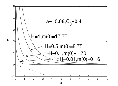
Figure 3: Several numerical breeze solutions with $L=0$ are shown as the solid curves with parameters $H=1,\ 0.5,\ 0.1,\ 0.01$ and corresponding $m(0)=17.75,\ 8.75,\ 1.70,\ 0.16$ at $a=-0.68$ and $C_{0}=0.4$. The straight dashed line passing through the origin is the sonic critical line. Near the core, all solutions approach the asymptotic free-fall behaviour (see equation 58) at small $x$.

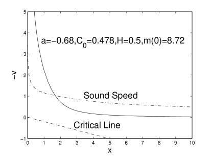
Figure 4: A comparison of $-v(x)$ solution with the sound speed $c(x)$ in the flow. Relevant parameters are: $a=-0.68$, $C_{0}=0.478$, $H=0.5$, $m(0)=8.72$. The dashed line is the sonic critical line. The solid line is the numerical solution of $-v(x)$ while the dash-dotted line represents the sound speed in the laboratory framework. The solution $-v(x)$ goes from subsonic at large $x$ to supersonic at small $x$.

Table 1: Parameters adopted for examples of numerical solutions are summarized in this Table 1. All these solutions do not encounter the sonic critical line. Using the standard Runge-Kutta scheme of fourth order with initial values calculated from the asymptotic solutions (48) at a sufficiently large $x$ (e.g., at $x=100$ in our numerical integrations). Integrating back towards the origin, we match the free-fall asymptotic solution (58) as $x\rightarrow 0^{+}$ and estimate the values of $m(0)$ relevant to central mass and mass accretion rate.

$a$	$C_{0}$	$H$	$K$	$L$	$m(0)$
$-0.68$	0.4	2.0	$-13.46$	0	36.0
$-0.68$	0.5	2.0	$-8.33$	0	35.8
$-0.68$	0.6	2.0	$-3.20$	0	35.6
$-0.68$	0.4	1.5	$-10.99$	0	26.8
$-0.68$	0.4	1.0	$-6.73$	0	17.7
$-0.68$	0.4	0.6	$-4.04$	0	10.5
$-0.68$	0.4	0.2	$-1.35$	0	3.44
$-0.68$	0.4	0.01	$-0.067$	0	0.162
$-0.67$	0.4	0.001	$-0.041$	0	0.0661
$-0.70$	0.4	1.0	$-1.56$	0	7.32
$-0.72$	0.4	1.0	$-0.62$	0	4.59
$-0.74$	0.4	1.0	$-0.30$	0	3.29
$-0.67$	0.4	0.001	$-0.041$	0.2	0.0651
$-0.68$	0.5	1.0	$-4.16$	0.2	17.6

We adjust the solution parameters $H$ and $L$ and the relevant parameters $a$ and $C_{0}$ to explore various solutions (see Fig. 3). When a solution goes back towards the origin, it matches with asymptotic free-fall solution (58) and gives the corresponding $m(0)$ value. For $a=-1$ in expression (48), solutions with $L=0$ have vanishing velocities at infinity; solutions with $L>0$ and $L<0$ correspond to constant outflows and inflows at infinity, respectively. Such solutions offer the following scenario: at the beginning time ($t=0$), the gas system is stationary or has a velocity outwards or inwards with its mass density profile proportional to $r^{2/a}$. Under the joint action of self-gravity and thermal pressure force, the entire system evolves into a central collapse eventually. Around the central region, the inward self-gravity is always larger than the thermal pressure force so that materials are accelerated towards the centre. Nothing singular happens as the local flow speed reaches the local sound speed (see Fig 4). When approaching the centre, the fluid is almost in a free-fall state. Because of our presumed spherical symmetry, something must happen around the centre to destroy the similarity flow or spherical symmetry. For example, a strong radiation shock may emerge surrounding the centre. Or, a black hole may take all accreting materials in.

The isothermal expansion-wave collapse solution (EWCS) of Shu (1977) was regarded as a limit for a family of solutions without encountering the sonic critical line. In other words, at a particular critical point $x_{e}$ along the sonic critical line, one of the two eigensolutions leads to the static singular isothermal sphere (SIS) while the other leads to a solution matching the central free-fall solution. Thus a semi-complete global solution with a weak discontinuity is constructed, connecting the two eigensolutions at $x_{e}$, with a static SIS for $x>x_{e}$. Similarly, for a particular pair of $a$ and $C_{0}$ values (see equation 37), a static SPS with $\gamma=4/3$ exists so that we can also construct the counterpart of isothermal EWCS. As every point $x$ is equivalent in the sense of the scaling invariance (35), we simply take $x_{e}=1$ without loss of generality. For this special pair of $a=-0.68$ and $C_{0}=0.6623$, we have $k=0$ for the slope of the sonic critical line, and the two corresponding eigensolutions are $v_{1}=0$ and $v_{1}=3(1+5a/7)=1.54$. Using $v_{1}=0$ with its corresponding $\alpha_{1}$ to integrate outwards, we obtain the outer part of a SPS as the static outer envelope. Meanwhile, using $v_{1}=3(1+5a/7)=1.54$ to integrate back towards the centre, we obtain a central free-fall solution. Together, we have constructed a polytropic EWCS with $\gamma=4/3$ (see Fig. 5).

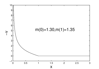
Figure 5: The polytropic EWCS with $\gamma=4/3$. The point of weak discontinuity is $x_{e}=1$. The outer part of the system is static SPS while the inner part approaches the free-fall asymptotic solution. The enclosed mass at the centre $m(0)$ is around $1.30$ and the collapsing mass $m(1)$ is around $1.35$, indicating that the majority of materials, around $96.3\%$ concentrates in the centre. Such polytropic EWCS of $\gamma=4/3$ exists only for $k=0$ with a pair of parameters $a=-0.68$ and $C_{0}=0.6623$.

Let us consider the enclosed mass $m(x)$, where $m(0)$ is the point mass at the centre and $m(1)-m(0)$ is the mass collapsing towards the centre. Our numerical result is $m(0)=1.30$ and $m(1)=1.35$. That is, $96.3\%$ of the total mass concentrates in the central object and only $3.7\%$ is collapsing towards the centre.

We can also construct other semi-complete global solutions without encountering the sonic singular surface. Starting from quasi-static solution (65) and (66) at small $x$ with $k=0$ and $V>0$ in equation (65), straightforward numerical integrations lead to global semi-complete solutions without encountering the sonic singular surface. Figure 6 shows such examples at $a=-0.68$ with a corresponding $C_{0}=0.6623$. These solutions never vibrate towards small $x$ according to our analysis (i.e., no complex conjugate roots are possible). With increasing $x$, they approach asymptotic expansion solution (51) and (52) rapidly. Numerical results indicate that with a $V>0$, the gas begins to flow outwards and approaches a constant density. The larger the value of $V$ is, the stronger the perturbation is, and the more rapidly the solution approaches the Einstein-de Sitter expansion phase with $v=2x/3$.

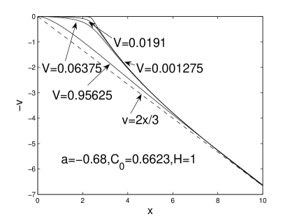
Figure 6: Four quasi-static numerical solutions with $k=0$ and $V>0$ in quasi-static asymptotic solution (65) for small $x$. The scaling parameter is $a=-0.68$ and the corresponding $C_{0}=0.6623$ is computed from equation (37). The parameter $B$ in the static solution is set to $1$. By these numerical solutions, it is clear that the larger the $V$ is, the more rapidly the solution is in the aberrance of the static state and approaches the Einstein de Sitter solution (51) and (52). The straight dashed line is $v=2x/3$ for the Einstein-de Sitter expansion.

Using new asymptotic solution (61) at small $x$, we can also construct global semi-complete solutions. As the sonic critical line is not enough to describe the relative position between numerical solutions and the sonic singular surface, we define a velocity $v_{c}$ such that

$$v_{c}\equiv-\big{(}\gamma C_{0}m^{2/3}\alpha^{1/3}\big{)}^{1/2}-ax\ ,$$ (85)

to represent a $v_{c}$ curve on the singular surface, depending upon the solution for the reduced enclosed mass $m(x)$ and mass density $\alpha(x)$ together with adopted parameters $C_{0}$, $a$ and $\gamma=4/3$. The purpose is to compare solution $v(x)$ against $v_{c}$ for the possibility of encountering the sonic singular surface. From this definition, it is easy to see that if a solution $v(x)$ meets the sonic singular surface at some point, this point must the intersection of the solution curve $v(x)$ and the $v_{c}$ curve thus defined. In equation (61), $R,\ N$ and $\lambda$ are three parameters to be determined. For an appropriate combination of these parameter values, the solution may not run into the sonic singular surface and eventually converge to asymptotic solution (51) and (52) at large $x$.

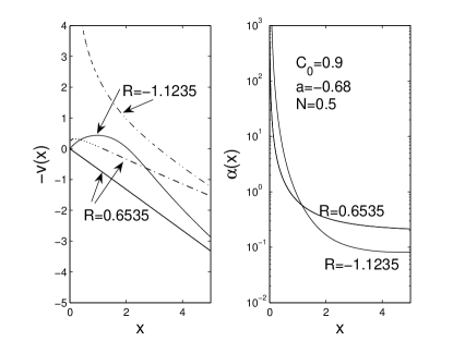
Figure 7: An example for the case of $a=-0.68$ and $C_{0}=0.9$ is illustrated. The corresponding slope $k=-0.3745$ for the sonic critical line. It has two real roots of $R$: one is $R=-1.1235$ and the other is $R=0.6535$. The inner part can be described by asymptotic solution (61) at small $x$ with other parameters $N=0.500$ and $\lambda=-2.9778$, while the outer part can be described by asymptotic solution (51) and (52) at large $x$ with parameter $\beta=-0.7362$. The two dash-dotted curves in the left panel are $v_{c}(x)$ as defined by expression (85) related to the relevant solutions.

This solution gives the following scenario: the central region is occupied by a high-density core with an outside medium of constant density moving outward. Once the inner core begins to move towards the centre, the outer part decelerates to 0 and also begins to move inwards. We also see that the mass density decreases rapidly as $x$ becomes large. Figure 7 shows a pair of such examples.

5.2 Solutions crossing the Straight Sonic Critical Line Smoothly

Only eigensolutions along the sonic critical line, derived in subsection 4.3.2, can cross the sonic singular surface smoothly. To investigate their properties, we start numerical integration from the vicinity of a sonic critical point with initial values given by one of the relevant eigensolutions. The analysis here becomes much simpler in light of the scaling invariance transformation (35) and properties for every sonic critical point are the same and hence an arbitrary point $x$ can be chosen for a certain pair of $a$ and $C_{0}$ parameters. By solving for eigensolutions along the sonic critical line and then extending the eigensolutions globally by numerical integrations, we find that the two types of eigensolutions have qualitatively different properties. A type I solution approaches the free-fall asymptotic solution (58) in the inner part for small $x$ and has an outer asymptotic solution described by solution (51) and (52) at large $x$. The physical scenario is that initially the gas with a constant density has a tendency to move outwards, because of the thermal pressure against gravity. The gravity force competes with the thermal pressure and wins eventually as time goes on, and then the gas begins to decelerate and accelerate to collapse towards the centre. Now the self-gravity dominates the thermal pressure force completely so that materials approach a free fall and finally smash onto the central object.

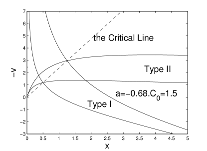
Figure 8: Two examples of semi-complete solutions crossing the straight sonic critical line in two possible eigendirections with parameters $a=-0.68$ and $C_{0}=1.5$. The sonic critical line is represented by the straight dash-dotted line with a negative slope $k=-2.3754$. The solid curves are the possible eigensolutions crossing the sonic critical line, one of which is at $x=0.5$ and the other is at $x=1.25$. The two eigensolutions approach different inner and outer asymptotic solutions described previously. Because of the scaling invariance of the ODEs, these two eigenproblems and the corresponding eigensolutions are actually the same. Take the eigenproblem at $x=1.25$ for example. Type I solution approaches equation (58) with $m(0)=38.4$ near the centre and has an outer asymptotic solution described by equation (52) and (51) with parameters $\beta=-1.6204$, $E=0.086$ and $F=-0.785$. Type II solution approaches equation (61) at small $x$ with parameters $\lambda=-3.00$, $R=-7.90$ and $N=0.179$. For large $x$, its behaviour can be represented by equation (48) with $H=2.055$ and $L=-11.392$. Please note that for $a>-1$, $-v(x)$ of a Type II solution always vanishes at large $x$; in this case of $a=-0.68$, the leading term of $-v(x)$ at large $x$ scales as $x^{-0.47}$.

In contrast, a type II solution has a quite different behaviour. In the vicinity of the origin, the velocity vanishes while the mass density diverges as described by asymptotic solution (61) around small $x$, while flow behaviour at large $x$ can be described by asymptotic solution (48). Based on the value of $C_{0}$ compared with the critical value of $2^{4/3}/6$, which determines whether $R$ has real roots, Type II solutions can be divided into two subtypes. Subtype I: For $C_{0}\geq 2^{4/3}/6$ corresponding to the existence of real roots of $R$, Type II solutions will approach $x=0$ as described by asymptotic solution (61). A special case is the SPS solution with $\gamma=4/3$ when $k=0$. One can prove that the value of $C_{0}$ for $k=0$ is not smaller than $2^{4/3}/6$. As discussed earlier, EWCS with $\gamma=4/3$ can be constructed here by connecting two branches of the two eigensolutions along the sonic critical line with $k=0$. These subtype solutions describe the following scenario. The outer part of the fluid system has a common flow behaviours which can be an inflow, or an outflow, or even a static envelope, while in the inner part, the pressure force and self-gravity compete with each other such that the magnitude of the radial speed remains finite and eventually vanishes at the centre. Subtype II: $C_{0}<2^{4/3}/6$ so that asymptotic solution (61) does not exist. A numerical integration backwards would be truncated before $x$ becomes sufficiently small. Physically, the enclosed mass $m(x)$ is related to the factor $ax+v$ by equation (27). Thus if $v(x)$ curve occasionally approaches the straight line $ax+v=0$, then there is no material inside this ‘radius’ $x_{v}$. In other words, a spherical void surrounds the centre and expands as time goes on in a self-similar manner. For $a<-1$ cases, the boundary of such a spherical void expands with deceleration and the edge radius is proportional to $t^{-a-1}$. From ODEs (8)$-$(12), the behaviours of density, velocity and pressure can be deduced. The enclosed mass within that point is zero, the reduced density $\alpha$ is finite, the reduced pressure $p$ approaches zero there, and the pressure gradient $dp/dx=-a(a+1)\alpha$ remains finite according to equation (10). Equation (11) requires the following limit

$$\lim_{ax+v\rightarrow 0}\frac{(ax+v)}{\alpha}\frac{d\alpha}{dx}=-\frac{2(2+a-\gamma)}{\gamma}\ ,$$ (86)

and it follows from equation (12) that

$$\frac{dv}{dx}=2(1+a)+\frac{2(2+a-\gamma)}{\gamma}\$$ (87)

remains finite there. Numerical results also confirm the situation that the enclosed mass $m(x)$ becomes $0$ before $x$ reaches the origin. An example of $a=-0.68$ and $C_{0}=0.3$ is shown in Figure 9

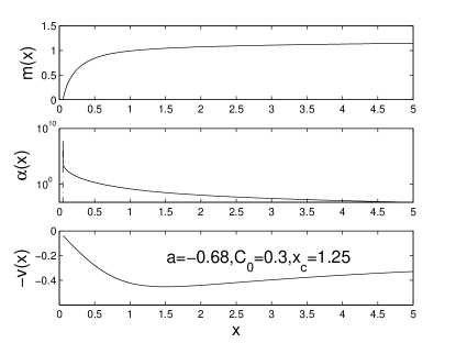
Figure 9: When $C_{0}$ is below $2^{4/3}/6\cong 0.42$, the asymptotic solution (61) no longer exists. The type II eigensolution is truncated before $x=0$. This figure shows an example of such behaviour. The relevant parameters are $a=-0.68$ and $C_{0}=0.3$ with the corresponding slope $k=0.3571$ for the sonic critical line. We obtain eigensolutions across the sonic critical line at $x_{c}=1.25$. Apparently, the enclosed mass becomes 0 before $x$ reaches the origin, i.e., in the $-v$ versus $x$ diagram, the velocity curve meets the line of $ax+v=0$ where the solution is truncated.

for the reduced quantities, such as $m(x)$, $\alpha(x)$ and $-v(x)$ in top, middle, and bottom panels respectively. This shows the real possibility of a spherical void occupying the central region of a certain astrophysical system (e.g., clouds, bubbles, planetary nebulae, stars or supernova remnants etc.) during its evolution under joint action of thermal pressure and self-gravity. Previously, Goldreich & Fillmore (1984b) discussed collisionless particles with self-gravity in an Einstein-de Sitter expanding universe. Steep perturbations can give rise to voids surrounded by overdense shells with sharp edges. Our preliminary results here show that in addition to the expansion of universe, a spherical matter system with thermal pressure against self-gravity can also lead to the formation of a central spherical void with an overdense shell along a sharp edge.

5.3 Self-Similar Flow Solutions with Shocks

Global behaviours of eigensolutions crossing the sonic critical line have been explored numerically. Starting from the two eigensolutions on the sonic critical line and integrating towards small $x$, one will approach the free-fall asymptotic solution (58) and the other will approach the new asymptotic solution (61) (see solution examples in Fig. 8). Type II solutions in Fig. 8 touch the sonic critical line twice. Other than this special situation, due to the scaling invariance property, we are unable to construct any global solutions across the sonic critical line twice smoothly which are possible in the isothermal cases of Lou & Shen (2004) and the conventional polytropic cases of Lou & Wang (2006).

In this subsection, we turn our attention to self-similar flows with shocks. From now on, subscripts $1$ and $2$ represent upstream and downstream sides of a shock, respectively. In particular, we use $C_{1}$ and $C_{2}$ to represent $C_{0}$ of the upstream and downstream sides, respectively. Because it involves local sound speed with respect to the shock reference framework in both upstream and downstream sides, we also calculate the corresponding sound speed $c_{s}\equiv(\gamma P/\rho)^{1/2}=(\gamma C_{0}m^{2/3}\alpha^{1/3})^{1/2}$ for each branch of solutions.

We begin with free-fall core collapse solutions.

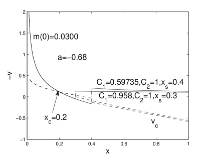
Figure 10: Two shock flow solutions are illustrated here. These solutions connect free-fall asymptotic solution at the inner part (small $x$) with an inflow or contraction at infinity (large $x$). The solid curves in the figure presents solutions and the dashed curves are corresponding curves of $v_{c}$ defined in equation (85). The scaling index $a=-0.68$. The two solutions share the same downstream branch with the free-fall solution parameter $m(0)=0.030$ and $C_{2}=1.00$ and it crosses the sonic critical line smoothly at $x_{c}=0.2$. The upstream side shows an inflow described by equation (48), with a set of parameters $\{C_{1},x_{s},H,L\}$. Two example solutions correspond to $\{0.5973,0.40,0.0019,-0.1322\}$ and $\{0.9580,0.30,0.0019,-0.1246\}$.

From the discussion of collapse solutions without crossing the sonic singular surface, any of this kind solution will cross the sonic singular surface even number of times, either smoothly or by shocks. By inspecting this topological characteristics and considering the simplest case of a single shock, we infer that this type of solutions, with shock jumps across the sonic singular surface, should be also possible to cross the sonic critical line smoothly at some critical point. Based on this observation, we specify a type I eigensolution at a given sonic critical point and integrate away from it in both directions. Let us take solutions shown in Figure 10 as examples of illustration. In the comoving reference framework of the shock, the outer part is supersonic and is thus the upstream side, and the inner part is the downstream side. Here we apply the matching procedure in the $\alpha-v$ phase diagram introduced by Hunter (1977). A notable differece from the case of $\gamma\neq 4/3$ is that the value of $C_{0}$ and the shock position will affect the value of $C_{0}$ and thus the sonic singular surface in the other solution branch. We also have a considerable freedom to construct a shock in one solution at a chosen place and then integrate forward. Such a numerical solution may approach a certain asymptotic solution, or it may encounter the sonic singular surface. Remember that when a numerical integration is from the downstream side to the upstream side, the square of the Mach number ${\cal M}_{2}^{2}$ of the downstream side should be within the range of $(0.125,1)$ and thus the shock position $x_{s}$ must be in a corresponding range. The $x_{s}$ value in the example of Figure 10 is around $0.4578$. This kind of gravitational core collapse solutions together with other solutions investigated previously, such as Shu (1977) and Lou & Shen (2004), may describe a possible stage of star formation in molecular clouds.

Tsai & Hsu(1995), Shu et al. (2002) and Bian & Lou(2005) connected the outer singular isothermal sphere (SIS) solution with either LP type solution or free-fall solution in the inner region by shocks in an isothermal gas. Using the matching procedure in the $\alpha-v$ phase diagram, shock flow solution of this kind with the free-fall asymptotic solution at small $x$ also exists in our polytropic case of $\gamma=4/3$.

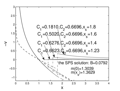
Figure 11: Examples of inner free fall and shock jumps to the SPS outer part and other asymptotic flow solutions far away. For the SPS shock connection, the shock is located at $x_{s}=1.23$ with $C_{1}=0.6623$ and $C_{2}=0.6696$ and the inner solution crosses the sonic singular surface again at $x_{c}=0.992$ smoothly. The mass at the centre is $m(0)=1.3039$ and the mass enclosed within the shock front is $m(x_{s})=1.3629$. For the three outer asymptotic flow solutions from the top in order, we have relevant shock parameters $\{C_{1},\ C_{2},\ x_{s}\}$ to be $\{0.1810,\ 0.6690,\ 1.8\}$, $\{0.5020,\ 0.6690,\ 1.6\}$, $\{0.6276,\ 0.6690,\ 1.4\}$, respectively, and relevant flow parameters $\{H,\ L,\ K\}$ of asymptotic solution (48) to be $\{0.082,\ -0.1,\ -1.0\}$, $\{0.080,\ 0.0,\ -0.3\}$, $\{0.080,\ 0.0,\ -0.07\}$, respectively (see asymptotic solution 48).

This particular kind of shock solutions depicts the following scenario. Initially the outside gas is in a radial force balance and the collapse starts from the central core region. Effects such as changes in the centre propagates outwards in the form of a self-similar shock. Materials are blown out by this shock. Because the gravity is stronger than the pressure force, materials eventually stop moving outwards and fall towards the centre.

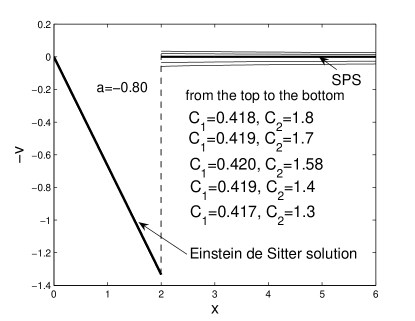
Figure 12: This figure illustrates a special case (the heavy solid line) of shock solution which connects the inner Einstein-de Sitter solution and the outer SPS with $\gamma=4/3$. Here, $C_{2}=1.58$ and the corresponding value of $a$ is $-0.80$. This kind of solutions may be regarded as a limiting solution as $C_{2}$ approaches $1.58$ while keeping $a$ the same. Also shown in this Figure are different upstream solutions of $C_{2}=1.3,\ 1.4,\ 1.7,\ 1.8$, respectively. For these four upstream solutions away from the SPS, the three relevant parameters $\{H,\ K,\ L\}$ for asymptotic solution (48) are $\{0.134,\ -0.007,\ 0.068\}$, $\{0.126,\ 0.00,\ 0.041\}$, $\{0.106,\ 0.00,\ -0.024\}$ and $\{0.101,\ 0.00,\ -0.041\}$, respectively.

While all LP type asymptotic solutions degenerate to the Einstein-de Sitter solution in our case of $\gamma=4/3$, shock solutions can also be constructed to connect the inner Einstein de Sitter solution with an outer SPS (see Fig. 12). Naturally, the outer SPS part is the upstream side with $v_{1}=0$, and the inner Einstein-de Sitter solution is the downstream side with $v_{2}=2x_{s}/3$ and $\alpha_{2}=2(1+2\sqrt[3]{3}C_{2})^{-1}/3$ at $x_{s}$ where $C_{2}$ is set to an appropriate value. Using $v_{2}$, $\alpha_{2}$ and $C_{2}$, we can express $v_{1}$ in terms of the scaling index $a$. The condition of $v_{1}=0$ then appears as a quadratic equation of $a$, which needs to be solved for $a$ with $a<-2/3$. Once this is done, we use $v_{2}$, $\alpha_{2}$, $C_{2}$ and the relevant root(s) of $a$ to calculate the Mach number ${\cal M}_{2}$ on the downstream side to check whether the requirement $1/8<{\cal M}_{2}<1$ is met. Once everything is complete and consistent, one of this kind of shock solutions is then constructed. We show an example here in Figure 12 with $C_{2}=1.5,\ a=-0.799,\ \alpha_{2}=0.1252$, leading to $C_{1}=0.383,\ \alpha_{1}=0.0207$ correspondingly, where the self-similar shock position $x_{s}$ can be any positive values because of the scale invariance property.

Shocks can also be inserted to connect the only two analytic solutions available, namely, the static SPS solution outside and the Einstein-de Sitter solutions inside. To construct this kind of shock solutions, the upstream quantities are $v_{1}=0$ and $\alpha_{1}=Bx_{s}^{2/a}$ with $C_{1}$ (i.e., the upstream $C_{0}$) satisfying conditions (36) and (37) for the existence of SPS, while the downstream quantities are $v_{2}=2x_{s}/3$ and $\alpha_{2}=2/[3(1+2\sqrt[3]{3}C_{2})]$ from the Einstein-de Sitter solution (38). With these constraints, it is straightforward to determine $C_{2}=1.58$, $C_{1}=0.42$ and $a=-0.80$. Figure 12 shows this solution with the shock position at $x_{s}=2.0$. It is easy to see from the figure that this solution represents the limiting solution of a solution family of $C_{2}$ approaching $1.58$ with $K=0$. It is unlike the isothermal results of Tsai & Hsu (1995) where this kind of solutions is a limit of a family of breeze solutions (Shu et al. 2002). Instead, it is a critical state to distinguish asymtotic outflow and inflow solutions. For $C_{2}$ being slightly larger than $1.58$, the asymptotic solution represents an inflow, while for $C_{2}<1.58$ the asymptotic solution corresponds to an outflow. In fact, this Einstein-de Sitter shock model can be applied to an explosion process with a stellar interior as an alternative of the rebound shock model of Lou & Wang (2006, 2007) described at the beginning of the next paragraph. The major difference here is a constant density within the shock front instead of being a diverging density near the centre; outside the shock front, the density approaches a power-law scaling with either infalling or outgoing stellar materials. When this shock front reaches the photosphere of the progenitor, we start to see observable effects of a supernova in optical bands.

Lou & Wang (2006) utilized a self-similar polytropic model to construct the gravitational core collapse and rebound shock processes in supernova explosions. Their conventional polytropic model solution with $\gamma\neq 4/3$ is to connect quasi-static solutions at small $x$ with outer asymptotic flow solutions at large $x$ by outgoing shocks. That model was recently generalized to include a random magnetic field using a magnetohydrodynamic (MHD) approach and to explore the origin of strong magnetic fields of compact objects (Lou & Wang 2007; Wang & Lou 2007). Based on our model framework here, this can also be done for a general polytropic gas with $\gamma=4/3$ and thus $q=2/3$. Starting numerical integrations both from the centre and from infinity (actually a sufficiently large $x$) and choosing a proper meeting point to match solutions in the $\alpha-v$ phase diagram, we adjust the shock position and parameters of outer asymptotic solution (48) to construct sensible solutions (e.g., Lou & Shen 2004).

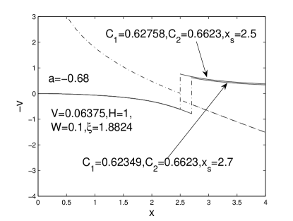
Figure 13: Shock solutions with quasi-static asymptote of equation (65) and (66) at small $x$ are shown here. The power index parameter $a$ is $-0.68$. In the downstream side, we use the same quasi-static solution while two uptream branches are different. The parameters in the downstream side for the quasi-static solution are $C_{2}=0.6623,\ B=1.00,\ W=0.10,\ V=0.06375,\ \xi=1.8824$. The upstream branch converges to asymptotic solution (48) at large $x$. Thus each upstream solution can be identified by a set of parameters $\{C_{1},\ x_{s},\ H,\ L\}$, where $x_{s}$ is the shock location and the last two are the coefficients in asymptotic solution (48). In this illustration the two sets of parameters are $\{0.62758,\ 2.5,\ 1.0096,\ -0.5323\}$ and $\{0.62349,\ 2.7,\ 1.0149,\ -0.4486\}$. The dash-dotted curves are corresponding segments of $v_{c}$ curve defined by condition (85).

Alternatively, instead of the above matching procedure, we can also start a numerical integration from the vicinity of the centre and then choose a certain point as the shock location. Shock jump conditions (75)$-$(77) determine all physical variables on the upstream side of a shock. A further numerical integration outwards until $x$ is sufficiently large completes the solution construction procedure. Using the numerical solution thus obtained, we can match with asymptotic solutions to determine relevant parameters. We find that the self-similar shock position can only exist within a finite interval of $x$ (e.g., in the case of $a=-0.68$, the self-similar shock position falls within the range of $1.3\leq x_{s}\leq 4.23$). Outside this interval of $x$, the square of Mach number ${\cal M}_{2}^{2}$ on the downstream side would be smaller than $1/8$ which is unphysical by our analysis on self-similar shock conditions. This $\gamma=4/3$ rebound shock model for supernovae may be more appropriate in certain aspects. During the initial phase for the emergence of a rebound shock in the dense stellar core, neutrino pressure, radiation pressure and gas pressure together may be modelled by a polytropic mixture of $\gamma=4/3$. The diverging density near the centre is expected to create a highly degenerate core there.

We also construct shocks connecting asymptotic solutions (48) at infinity and (61) near the centre.

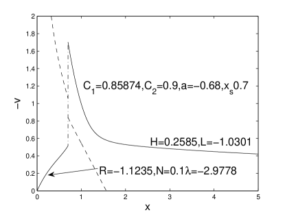
Figure 14: A similarity shock solution with $a=-0.68$ and $C_{1}=0.85874,\ C_{2}=0.9$ is illustrated. It connects asymptotic solution (48) with parameters $H=0.2585,\ L=-1.0301$ and asymptotic solution (61) with parameters $R=-1.1235,\ N=0.1,\ \lambda=-2.9778$. The solid curve represents the shock solution and the dashed curve represents corresponding segments of $v_{c}$ curve defined by condition (85).

In the above analysis, we know that the inner part of this solution can only appear in the first quadrant in the plane of $-v$ versus $x$. The numerical treatment starts from the centre and goes outwards. Before the solution meets the sonic singular surface, jump conditions are included to introduce a shock across the sonic singular surface. We then continue to integrate outwards until $x$ is sufficiently large to match with asymptotic solutions at large $x$. Numerical experiments show that almost all such solutions match asymptotic solution (48), in which mass density and flow velocity both converge. It is also possible that after a shock jumping across the sonic singular surface and integrating outwards, the radial flow velocity decreases rapidly so that it crashes onto the sonic singular surface again. In our numerical experiment, we do not find solutions with twin shocks or others, which jump across the singular surface twice or more (see Bian & Lou 2005).

6 Discussion and Conclusions

We have explored and examined the similarity flow solution structures in a general polytropic gas with a polytropic index $\gamma=4/3$. Previously, Goldreich & Weber (1980) considered a special case of $\gamma=4/3$ with a constant specific entropy. By their assumptions and analysis, only homologous collapse solutions exist by invoking the time reversal invariance, i.e., the radial flow velocity $u$ takes on the form of $2r/(3t)$ until the mass density vanishes at a certain point. Yahil (1983) mentioned the case of Goldreich & Weber (1980) as a special limit. In reference to earlier work and based on a self-similar transformation, we systematically examined the case of $\gamma=4/3$ with specific entropy conservation along streamlines. We have substantially generalized the earlier analyses, discovered new asymptotic solutions, and constructed various self-similar solutions without or with shocks.

In reference to earlier analyses of Goldreich & Weber (1980) and Yahil (1983), our model framework mainly focuses on $\gamma=4/3$ with the conservation of specific entropy along streamlines, which is more general and perhaps, closer to reality than the conventional polytropic gas of a constant specific entropy everywhere at all times. Of course, the case of a constant specific entropy is also possible and can be properly accommodated and treated within our polytropic model framework of $\gamma=4/3$. Under our more general formalism, we extend the work of Goldreich & Weber (1980) and obtain many interesting results. The solutions are divided into two broad classes: solutions with $a=-2/3$ precisely belong to Class I and solutions with $a<-2/3$ belong to Class II. For the situation of $-2/3<a<0$ as mentioned at the beginning of deducing asymptotic behaviours, the divergent velocity at large $x$ is not of interest and hence we only consider two classes I and II solutions.

Class I solutions are characterized by $P\propto\rho^{4/3}$ with the proportional coefficient related to the specific entropy being an arbitrary function of $x$, while for Class II solutions, this proportional coefficient depends on the enclosed mass $M$ in a power-law form. We discuss these two classes separately.

6.1 Class I Self-Similar Solutions

Class I self-similar solutions represent a substantial extension of the special solutions with a constant entropy derived by Goldreich & Weber (1980). For an astrophysical system such as stars, the specific entropy is not expected to be a global constant in general. For a stellar interior, this depends on the competition between thermal kinetic energy and Fermi energy as determined by the mass density. Qualitatively speaking, especially for a compact object, the closer to the centre, the closer the material is in a degenerate state; this would correspond to a smaller specific entropy. However, the density is relatively small and the temperature is relatively low in the outer part of a star, perhaps also leading to a lower level of entropy. We do not yet know the exact distribution of specific entropy within a star so far. Thus the case of a constant entropy is the simplest to consider and provides a certain sense for a homologous dynamic process. The model analysis of this paper is more general and allows for a fairly arbitrary distribution of specific entropy along streamlines. Meanwhile, the radial velocity profile remains always equal to $2r/(3t)$. For a given time $t$, the radial velocity increases linearly with increasing radius $r$. Hence, this solution can be valid within a finite radial extent. It turns out that the mass density vanishes at some place referred as the outer boundary of the flow system.

According to the model analysis of Goldreich & Weber (1980), a pre-collapse progenitor star of a static configuration may evolve into a homologous core collapsing phase (see Figure 1), when the pressure suddenly decreases by a fraction within a range of $\sim 2.9\%$. Early simulations of Bethe et al. (1979) indicated a substantially larger pressure reduction of $26\%$ is needed in order to initiate collapse in supernova explosions. The much smaller fraction change of pressure reduction for a homologous core collapse given by Goldreich & Weber (1980) is actually related to the assumption of a constant specific entropy (i.e., their constant $\kappa$) in space and time. Requiring specific entropy conservation along streamlines and allowing the specific entropy to be a function of space and time, it is possible to have a homologous core collapse for a much larger fractional change of pressure reduction. In our more general analysis and notations, we find that other forms of $g(x)$ instead of $g(x)=1$ can give rise to a fractional change of $26\%$ or larger for a pressure reduction. Physically, this corresponds to different distributions of specific entropy along streamlines.

To illustrate this case specifically, we choose $g(x)=1/(1+\epsilon x)$ where $\epsilon>0$ is an adjustable parameter to gradually modify the shape of $g(x)$. When $x$ is sufficiently small, $g(x)$ is nearly equal to $1$, analogous to the $g(x)=1$ case. Globally $g(x)$ is a decreasing function with increasing $x$. When $\epsilon$ is small, $g(x)$ decreases slowly and only deviates from $g(x)=1$ case when $x$ is sufficiently large. For large $\epsilon>0$, the result will differ considerably from that of Goldreich & Weber (1980). We carry out such a $g(x)$ experiment numerically.

Substituting dimensional quantities into the dimensionless state function $p=g(x)\alpha^{4/3}$, the dimensional equation of state can be written explicitly as

$$P=\frac{g(x)}{A^{2}}(4\pi G)^{1/3}\rho^{4/3}\ ,$$ (88)

where for a given time $t$, $g(x)$ corresponds to a radial distribution of specific entropy. Parameter $A$ also varies for different values of chosen $f(0)$ for a certain system in which the total enclosed mass $M$ is conserved and thus the value of $A$ parameter can be deduced from equation (25). The variation in $A$ value actually corresponds to the variation range for fractional change in pressure denoted by $r_{p}$; in Goldreich & Weber (1980), this $r_{p}$ is $2.9\%$ as $f(0)$ increases from $f_{c}$ to infinity. For any given form of $g(x)$, the limiting case is the Lane-Emden equation (e.g., Chandrasekhar 1939) as long as $g(x)\rightarrow 1$ as $x\rightarrow 0^{+}$. Of course, this applies to our chosen form of $g(x)=1/(1+\epsilon x)$ as $x\rightarrow 0^{+}$.

Table 2: When $g(x)$ takes the form of $1/(1+\epsilon x)$, the results are shown in Figure 15. As $f(0)$ is sufficiently large, the outer boundary at a finite $x$ where $f(x)=0$ is extremely small and thus $g(x)$ can be almost treated as a constant; these results vary little as compared with those of Goldreich & Weber (1980) for $f(0)\rightarrow+\infty$ corresponding to the Lane-Emden equation. Results in Figure 15 mainly focus on the limiting case of $f(0)\rightarrow f_{c}^{+}$. For possible $f(x)$ solutions of a homologous core collapse, we use $r_{p}$ to denote the range for fractional change of pressure variation as $f(0)$ increases from $f_{c}$ to infinity.

$\epsilon$	$f_{c}$	$\bar{\rho}/\rho_{c}$ at $f_{c}$	$r_{p}$
$0$	$4.67047$	$0.00655$	$2.9\%$
$0.01$	$4.58642$	$0.00693$	$3.6\%$
$0.05$	$4.28755$	$0.00848$	$6.4\%$
$0.1$	$3.98354$	$0.0106$	$10\%$
$0.3$	$3.23130$	$0.0198$	$26\%$
$0.5$	$2.83696$	$0.0293$	$42\%$

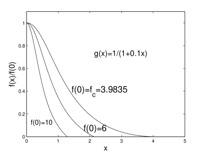
Figure 15: Results of the normalized $f(x)/f(0)$ is displayed for $g(x)=1/(1+0.1x)$ and $\epsilon=0.1$. In this case, the minimum of $f(0)$ is $f_{c}=3.9835$ for physical solutions.

Table 2 and Figure 15 show major results for a range of $\epsilon>0$ values. Numerical experiments indicate that as $\epsilon$ increases from $0$, the limiting value $f_{c}$ of $f(0)$ decreases while the density ratio $\bar{\rho}/\rho_{c}$ increases. More importantly, the range of fractional change $r_{p}$ by which the pressure can be reduced for a homologous core collapse becomes larger and larger. Table 2 shows that for $\epsilon=0.3$, we have $r_{p}\cong 26\%$; in other words, for such a large fractional change in pressure reduction (e.g., Bethe et al. 1979) in order to initiate supernovae, it is still possible for a homologous core collapse prior to the development of a rebound shock. It is conceptually important that a different specific entropy distribution of $g(x)$ from a constant value can lead to a better agreement with numerical simulations; this appears more effective than the inclusion of a less massive core in the centre as mentioned in Goldreich & Weber(1980).

6.2 Class II Self-Similar Solutions

In addition to extensions of Goldreich & Weber (1980) discussed in the above subsection, we also substantially generalize the self-similar solution space for $\gamma=4/3$ by adjusting the scaling index $a$. In contrast to $\gamma\neq 4/3$, a straightforward analysis with $\gamma=4/3$ leads to an exact value of $q=2/3$ that is independent of $a$. The dimensional equation of state then takes the form of $P\propto M^{2/3}\rho^{4/3}$ with a constant proportional coefficient. We can compare the thermal energy $k_{B}T$, where $k_{B}$ is the Boltzmann constant, with the Fermi energy $\varepsilon_{F}$. Neglecting the rest mass in the relativistic regime, the relationship between total energy $\varepsilon$ and momentum $\mathbbm{p}$ for a single particle can be written as $\varepsilon=c\mathbbm{p}$ where $c$ is the speed of light, leading to $\varepsilon_{F}\propto\rho^{1/3}$. In our model, the state function gives $k_{B}T\propto P/\rho\propto M^{2/3}\rho^{1/3}$. It follows that

$$\frac{k_{B}T}{\varepsilon_{F}}\propto M^{2/3}\ .$$ (89)

The enclosed mass $M$ is a non-decreasing function in radius $r$. At a given time $t$, we see from this relation that, at small $r$, the enclosed mass is small and hence this ratio is also small. Physically in the inner core of a star, where materials are highly condensed and may be close to a degenerate state, the specific entropy is low.

A modified self-similar transformation is introduced for $\gamma=4/3$. In the self-similar transformation for a conventional polytropic gas (i.e., $P=\kappa\rho^{\gamma}$ with globally constant $\kappa$ at all times), the sound speed appears either explicitly or implicitly. In contrast, we here use an integration constant $C_{0}$ relating to the sound speed and transformation (7) does not involve the sound speed because of the uniqueness of the $\gamma=4/3$ case; this $C_{0}$ coefficient is in fact allowed by the transformation and is an adjustable parameter in our analysis for astrophysical applications. At a deeper level, we realize that as the special self-similar transformation (7) for $\gamma=4/3$ does not involve the sound speed, we have a scaling invariance (35) which simplifies our theoretical analysis considerably.

By comparisons and analogies of solutions known for $\gamma\neq 4/3$, we try our best to find the counterpart solutions and to discover new solutions for $\gamma=4/3$. Global analytic solutions, i.e., static SPS solution (36) and (37) and Einstein-de Sitter expansion solution (38), still exist for $\gamma=4/3$ with some modifications. Analytic asymptotic solutions of various kinds are also derived for both large and small $x$. However, the LP-type solution no longer exists for $\gamma=4/3$ (thus $q=2/3$) except for rare situations, while other counterpart solutions are readily found. In addition, a new type asymptotic solution (61) is discovered in the regime of small $x$. It seems that this type of asymptotic polytropic solutions only exists for $\gamma=4/3$.

We have also examined properties of the sonic singular surface and the sonic critical line of coupled nonlinear ODEs (33). A salient feature of $\gamma=4/3$ case is that all sonic critical lines are straight and pass through the origin $x=0$ and $v=0$ in the $-v(x)$ versus $x$ presentation; while first revealed by extensive numerical experiments, these remarkable results can be proven analytically. It is also fairly straightforward to derive two eigensolutions to smoothly cross the straight sonic critical line. In later analyses, we realize that the sonic critical line cannot fully represents the behaviours of the sonic singular surface, especially for constructing shocks. We hence use $v_{c}(x)$ defined by equation (85) for each solution, which is another curve on the sonic singular surface and tightly relates to the current solution, to show the interrelation between the current solution and the sonic singular surface. According to definition (85), the solution meets the singular surface if and only if the solution and the corresponding $v_{c}$ intersects; meanwhile, a shock solution jumping across the sonic singular surface also jumps across the corresponding $v_{c}$ in $v(x)$ versus $x$ plane. The standard Runge-Kutta scheme (e.g., Press et al. 1986) is used to numerically integrate coupled nonlinear ODEs (33) and (34) to connect various asymptotic solutions and eigensolutions across the sonic critical line. We also construct possible solutions with and without shocks for potential astrophysical applications. From the behaviours of these semi-complete solutions, we can see that many such solutions have similar behaviours as those for $\gamma\neq 4/3$ in a qualitative manner. And our solutions can be sensibly regarded as limits of $\gamma\rightarrow 4/3$ when a polytropic gas becomes relativistically hot or degenerate. Our analysis for $\gamma=4/3$ does share a certain common characteristics with cases for $\gamma\neq 4/3$.

We can readily solve for eigensolutions crossing the straight sonic critical line. Once the slope $k$ of the sonic critical line is positive, we can construct a new type of self-similar solution characterized by an expanding central spherical void within which the enclosed mass is zero or negligible. Around the edge of such an expanding void, there exists an overdensed shell where the density variation becomes rather steep. Diffusion processes are expected to smooth out such relatively steep gradients locally. To consider properties of spherical void boundary, we first note that such a void expands with a radial speed

$$\dot{r}_{e}=-ar_{e}/t\qquad\quad\Rightarrow\qquad\quad r_{e}\propto t^{-a}\ ,$$ (90)

where $r_{e}$ stands for the radius of the spherical void edge. The spherical void edge evolves as a power law of time $t$ with a scaling index $-a$. One also notes by equation (86) that the density gradient approaches a negative infinity near the void edge. We expect that in a narrow region near the spherical void edge, materials are actually diffused instead of being so sharply distributed as shown by our solution mathematically. Within this narrow region, the local evolution does not behave self-similarly and may not be spherically symmetric, while the overall self-similar profile remains on large scales. In the outer part, the mass density scales as $\rho\propto r^{2/a}$ and the radial flow velocity remains finite with a wind. In fact, it is also possible to construct various shock solutions with a central void.

At this stage, we may outline a physical scenario in the context of a supernova explosion. During the core collapse of a progenitor, neutrons are formed in abundance and neutrinos of relativistic energies are released. In a high-density environment, neutrino opacity is extremely high so that neutrino pressure, radiation pressure and gas pressure work together to drive the central core expansion. In the relativistic regime, we may ignore tiny neutrino masses and regard the neutrino gas as polytropic with an index $\gamma_{n}=4/3$. Similarly, the radiation pressure resulting from the photon gas trapped in the stellar interior can also be regarded as polytropic with an index $\gamma_{\nu}=4/3$. In the hot stellar core of high temperatures, we may approximate the thermal gas pressure as polytropic with an index $\gamma_{p}\cong 4/3$. It might be conceivable that under certain situations, the neutrino pressure is so overwhelming such that a central void may start to form. As the outer part expands and density drops, neutrinos escape while the radiation and thermal gas pressures continue to drive the expansion. It should be emphasized that in real situations, a grossly spherical void may still encompass materials here and there but the mass density inside is substantially lower than that of surroundings.

In this context, we note the model work of Fillmore & Goldreich (1984b) who considered a collection of collisionless particles in an expanding universe of the Einstein-de Sitter form. There is no pressure effect from particles in their model. In essence, the background Einstein-de Sitter expansion prescribed is similar to the rapid expansion driven by the thermal pressure force in our model, both providing the tendency for particles to move outwards in competition with the inward self-gravity. The key physical difference is that the Einstein-de Sitter expansion of the universe is homogeneous (presumably driven by the ubiquitous dark energy) while our gas expansion is driven by the thermal gas pressure closely related to gas mass density and temperature. Not only in the case $\gamma=4/3$, self-similar void solutions can also be constructed for $\gamma\neq 4/3$ and isothermal gas which we shall investigate more thoroughly in separate papers.

Besides certain similarities with previous polytropic model analysis with $\gamma\neq 4/3$, the case of $\gamma=4/3$ carries its own unique features. First, because of scaling invariance (35), various self-similar solutions can be readily classified, especially for the two eigensolutions across the sonic critical line. Once solution properties at a chosen point $x$ have been examined completely, other points will have the same solution characteristics by scaling invariance (35). This simplifies the analysis to a considerable extent. Fundamentally, the cause of this scale invariance (35) is due to the fact that the sound speed is not involved in self-similar transformation (7). In various solutions, the case of $\gamma=4/3$ also shows some differences: (i) the LP type solution does not exist, except for rare situations (see Appendix B); (ii) when discussing the quasi-static solution at small $x$, two sensible roots may be found for $\gamma<4/3$ (see Lou & Wang 2006), while one of the two roots is always unacceptable for $\gamma=4/3$ with only one sensible root being available in our model calculations; (iii) it is no longer possible for a quasi-static solution at small $x$ to show a vibration behaviour here. The solution quickly converges to an outer asymptotic solution; and (iv) the sonic critical lines with constant density are straight lines emanating from the origin in the $-v(x)$ versus $x$ presentation.

6.3 Conclusions

To sum up this paper, we have explored possible self-similar solutions, both analytical and numerical, for a generalized polytropic gas with $\gamma=4/3$. The classical analysis of Goldreich & Weber (1980) for a constant specific entropy everywhere at all times is substantially extended by specific entropy conservation along streamlines with specific entropy dependent on time and space. This differs from what Yahil (1983) did in this context. In addition to counterparts of various previously known types of polytropic solutions with $\gamma\neq 4/3$, we find two new asymptotic solutions. One notable feature is that sonic critical lines are all straight lines emanating from the origin in the $-v(x)$ versus $x$ presentation with constant densities. Using all asymptotic solutions available, two eigensolutions across the sonic critical line and self-similar shock conditions, global semi-complete solutions are constructed numerically. Two classes of self-similar solutions are investigated separately according to the value of the scaling index $a$. For Class I solutions with $a=-2/3$ precisely, we can simulate the homologous evolution of a flow system once the distribution of specific entropy is prescribed. These more general solutions for a homologous core collapse (Goldreich & Weber 1980) may be utilized to model the dynamic formation of an inner compact core from a pre-collapse stellar interior. Collapsing solutions of Class II with $a<-2/3$ may also explain the formation of compact objects and other similar flow systems, while expansion solutions with shocks can be utilized to model supernova explosions (e.g., Lou & Wang 2006, 2007).

By equations (8)$-$(12), we emphasize several aspects of solutions for $(3a+2)=0$ and for $(3a+2)\rightarrow 0$. Based on our analysis, the Einstein-de Sitter solution with $\gamma=4/3$ exists for $(3a+2)\neq 0$, $(3a+2)\rightarrow 0$ and $(3a+2)=0$. Except for this special Einstein-de Sitter solution, Class I solutions valid for $(3a+2)=0$ cannot be obtained by taking the limit of $(3a+2)\rightarrow 0$ for Class II solutions. In other words, Class I and II solutions are qualitatively different solutions and we need to consider them separately. By equations (8) and (27) during the limiting process of $(3a+2)\rightarrow 0$, we must require $(ax+v)\rightarrow 0$ in order to have a finite reduced mass $m(x)$. Only the Einstein-de Sitter solution and Class I solutions with $(3a+2)=0$ bear this unique feature for the reduced flow speed $v(x)$ while all other Class II solutions are excluded by this limiting procedure.

In the course of investigation, we realize the possibility of constructing self-similar solutions for dynamic evolution of central spherical void in a flow system involving self-gravity and thermal pressure. Here, the thermal pressure force drives the gas expansion sufficiently fast and creates a central spherical void by pushing materials outwards. By specific examples, we now prove by analytical and numerical calculations that a spherical void can indeed form in astrophysical flow systems under the joint action of thermal pressure force and self-gravity. We expect that such processes could happen in association with supernova explosions and evolution of supernova remnants.

At the beginning of our model formulation, several physical effects, such as nuclear reactions, radiation pressure, neutrino transport, general relativistic effects, rotational effects and magnetic field, are not taken into account. Under various situations, these effects can be very important in real astrophysical systems. Given these approximations and idealizations of our model, it is still hoped that this simple theoretical model framework may catch certain essential characteristics or features of flow phenomena of relevant scenarios and interpretations.

Appendix A The explicit form of $v^{\prime}$ and $\alpha^{\prime}$

Using Cramer’s rule in equations (33) and (34), one can easily deduce the explicit forms of $v^{\prime}(x)$ and $\alpha^{\prime}(x)$, namely,

$$v^{\prime}(x)={\cal V}(x)/{\cal D}(x)\ ,$$ (91)

$$\alpha^{\prime}(x)/\alpha(x)={\cal A}(x)/{\cal D}(x)\ ,$$ (92)

where

$${\cal V}(x)\equiv-\frac{(ax+v)^{2}}{(3a+2)}\alpha+(a+1)(ax+v)v\qquad\qquad\qquad$$

$$-\left(6+3a-\frac{4v}{x}\right)\frac{2C_{0}}{3}\left(\frac{ax+v}{3a+2}\right)^{2/3}x^{4/3}\alpha\ ,\quad$$ (93)

$${\cal A}(x)\equiv 2(ax+v)\left(1-\frac{v}{x}\right)+\frac{(ax+v)}{(3a+2)}\alpha-(a+1)v\qquad$$

$$+\frac{2C_{0}}{3}\left(\frac{ax+v}{3a+2}\right)^{-1/3}x^{4/3}\alpha\ ,\qquad$$ (94)

$${\cal D}(x)\equiv(ax+v)^{2}-\frac{4C_{0}}{3}x^{4/3}\left(\frac{ax+v}{3a+2}\right)^{2/3}\alpha\ .\qquad\qquad$$ (95)

The sonic singular surface corresponds to ${\cal D}(x)=0$; together with either ${\cal V}(x)=0$ or ${\cal A}(x)=0$, the sonic critical line is then determined. Note that ${\cal V}(x)=0$ is equivalent to ${\cal A}(x)=0$ on the sonic singular surface.

Appendix B Existence condition for Larson-Penston type solutions

Starting from equations (8)$-$(12), we briefly discuss the existence of Larson-Penston (LP) type solutions for a general case of $a\neq-2/3$ without constraining $\gamma$. In fact, equation (12) is equivalent to equations (8) and (9). Assuming Taylor series expansions in the vicinity of $x=0$, we write the solutions as

$$v(x)=\sum_{k=0}^{\infty}v_{k}x^{k}\ ,\qquad\qquad\alpha(x)=\sum_{l=0}^{\infty}\alpha_{l}x^{l}\ ,$$ (96)

where $v_{k}$ and $\alpha_{l}$ are constant coefficients with $\alpha_{0}\neq 0$. By equation (9), the enclosed mass is given by

$$m(x)=\int_{0}^{x}y^{2}\alpha(y)dy=\sum_{l=0}^{\infty}\frac{\alpha_{l}}{(l+3)}x^{l+3}\ .$$ (97)

While from equations (8) and (9), we have

$$m(x) = \frac{(ax+v)}{(3a+2)}x^{2}\alpha$$ (98)

$$= \frac{x^{2}}{(3a+2)}\left(ax+\sum_{k=0}^{\infty}v_{k}x^{k}\right)\left(\sum_{l=0}^{\infty}\alpha_{l}x^{l}\right)\ .$$

The two expressions of $m(x)$ should be equal, giving rise to a series of relations among the coefficients of $\alpha(x)$ and $v(x)$,

$$v_{0}=0\ ,\qquad v_{1}=2/3\qquad\qquad\qquad$$ (99)

$$4(a+v_{1})\alpha_{1}+4v_{2}\alpha_{0}=(3a+2)\alpha_{1}$$ (100)

$$\vdots$$

Besides, the reduced pressure can also be written as a series expansion in the form of

$$p=C_{0}m^{q}\alpha^{\gamma}=C_{0}x^{3q}\left[\sum_{l=0}^{\infty}\frac{\alpha_{l}}{(l+3)}x^{l}\right]^{q}\left(\sum_{k=0}^{\infty}\alpha_{k}x^{k}\right)^{\gamma}\ .$$ (101)

Substituting all these series expansions into equation (10) and comparing coefficients of the same powers of $x$, we have the following conclusions. For an arbitrary $q$ in general, consider the power factor $x^{3q}$ in equation (101). If $3q$ is not an integer, the power index of every term in $p$ is not an integer, and the terms thus cannot have the same power of other terms in equation (10). Consequently, no such a series solution exists. A necessary condition for the existence of LP type solution is that $q$ takes the form of $J/3$ with $J$ being an integer. For example, $J=0,\ q=0$ and thus $a=\gamma-2$ and $C_{0}=1$, we can readily obtain the following asymptotic solution (equations 28a and 28b in Suto & Silk 1988), namely

$$v(x)=\frac{2}{3}x+\frac{\alpha_{0}^{1-\gamma}}{15\gamma}\left(\alpha_{0}-\frac{2}{3}\right)\left(a+\frac{2}{3}\right)x^{3}+\cdots\ ,$$ (102)

$$\alpha(x)=\alpha_{0}-\frac{\alpha_{0}^{2-\gamma}}{6\gamma}\left(\alpha_{0}-\frac{2}{3}\right)x^{2}+\cdots\ .\qquad\qquad$$ (103)

For $J=2,\ q=2/3$ and $p=C_{0}m^{2/3}\alpha^{4/3}$, one readily obtains

$$v_{0}=0\ ,\qquad\quad v_{1}=2/3\ ,\quad\qquad v_{2}=0\ ,\qquad\qquad\quad$$ (104)

$$\alpha_{0}=\frac{2}{3}\left(1+2\sqrt[3]{3}C_{0}\right)^{-1}\ ,\qquad\alpha_{1}=0\ .\qquad\qquad\qquad$$ (105)

For any given index integer $k>1$ in the series expansion, if we have already determined coefficients $\alpha_{i}$ and $v_{i+1}$ where $0\leq i\leq k-1$, a comparison of the coefficients of each side of ODEs (8) and (10) will give a pair of linear equations for $\alpha_{k}$ and $v_{k+1}$, which has a unique solution for $\alpha_{k}$ and $v_{k+1}$. Thus, coefficients $\alpha_{i}$ and $v_{i}$ ($i\geq 1$) have only one solution. On the other hand, $v_{i}=0$ and $\alpha_{i}=0$ ($i\geq 1$) gives a solution to this problem. Consequently for $q=2/3$, only the Einstein-de Sitter solution exists and no LP type of solution can be found. One possible yet rare exception occurs when the coefficient determinant of one of the linear equations for $v_{i}$ and $\alpha_{i}$ becomes zero. We do not give more calculations on these special cases in this paper.

Appendix C Requirement on $C_{0}$ for the existence of asymptotic solution (59)

We denote the left-hand side of equation (63) by $h(R)$ where $R<2/3$ is required by $\lambda<0$. For a sufficiently large value of $|R|$ with $R<0$, we have $h(R)>0$; and for $R\rightarrow 2/3^{-}$, we also have a positive $h(R)$. Taking the first derivative of $h(R)$ and setting it equal to $0$, we obtain only one root denoted by $R_{0}$, namely

$$R_{0}=(6C_{0})^{3/4}(3a+2)-a$$ (106)

for the minimum of $h(R)$. Therefore if $h(R_{0})$ is also larger than $0$, then equation $h(R)=0$ has no real roots and hence asymptotic solution (63) does not exist. On the other hand, if $h(R_{0})$ is smaller than zero, then equation $h(R)=0$ always has two real roots. The critical case of $h(R_{0})=0$ corresponds to a double root, and a critical value of $C_{0}=2^{4/3}/6\approx 0.4200$ is thus known.

References

- (1) Bethe H. A., Brown G. E., Applegate J., Lattimer J. M., 1979, Nucl. Phys., A324, 487
- Bian & Lou (2005) Bian F.-Y., Lou Y.-Q., 2005, MNRAS, 363, 1315
- Boily & Lynden-Bell (1995) Boily C. M., Lynden-Bell D., 1995, MNRAS, 276, 133
- (4) Boss A. P., Myhill E. A., 1992, ApJS, 83, 311
- Bouquet et al. (1985) Bouquet S., Feix M. R., Fijalkow E., Munier A., 1985, ApJ, 293, 494
- (6) Chandrasekhar S., 1939, An Introduction to the Study of Stellar Structure, Dover Publications, Inc., London
- (7) Chandrasekhar S., 1960, Radiative Transfer, Dover Publications, Inc., New York
- (8) Cheng A. F., 1977, ApJ, 213, 537
- Cheng (1978) Cheng A. F., 1978, ApJ, 221, 320
- Chevalier (1982) Chevalier R. A., 1982, ApJ, 258, 790
- (11) Curry C. L., McKee C. F., 2000, ApJ, 528, 734
- Fatuzzo et al. (2004) Fatuzzo M., Adams F. C., Myers P. C., 2004, ApJ, 615, 813
- (13) Fillmore J. A., Goldreich P., 1984a, ApJ, 281, 1
- (14) Fillmore J. A., Goldreich P., 1984b, ApJ, 281, 9
- (15) Foster P. N., Chevalier R. A., 1993, ApJ, 416, 303
- Goldreich & Weber (1980) Goldreich P., Weber S. V., 1980, ApJ, 233, 991
- Hunter (1962) Hunter C., 1962, ApJ, 136, 594
- Hunter (1977) Hunter C., 1977, ApJ, 218, 834
- Hunter (1986) Hunter C., 1986, MNRAS, 223, 391
- (20) Jijina J., Adams F. C., 1996, ApJ, 462, 874
- Landau & Lifshitz (1987) Landau L. D., Lifshitz E. M., 1987, Fluid Mechanics, 2nd edition, Pergamon Press, New York
- Larson 1969a (1969a) Larson R. B., 1969a, MNRAS, 145, 271
- Larson (1969b) Larson R. B., 1969b, MNRAS, 145, 405
- (24) Larson R. B., 1985, MNRAS, 214, 379
- Lou & Shen (2004) Lou Y.-Q., Shen Y., 2004, MNRAS, 348, 717
- Lou & Wang (2006) Lou Y.-Q., Wang W.-G. 2006, MNRAS, 372, 885
- (27) Lou Y.-Q., Wang W.-G., 2007, MNRAS, 378, L54
- Mclaughlin & Pudritz (1997) Mclaughlin D. E., Pudritz R. E., 1997, ApJ, 476, 750
- (29) Myers P. C., Bachiller R., Caselli P., Fuller G. A., Mardones D., Tafalla M., Wilner D. J., 1995, ApJ, 449, L65
- (30) Myers P. C., Mardones D., Tafalla M., Williams J. P., Wilner D. J., 1996, ApJ, 465, L133
- Penston (1969a) Penston M. V., 1969a, MNRAS, 144, 425
- Penston (1969b) Penston M. V., 1969b, MNRAS, 145, 457
- (33) Rybicki G.B., Lightman A.P., 1979, Radiative Processes in Astrophysics, John Wiley & Sons, New York
- Shu (1977) Shu F. H., 1977, ApJ, 214, 488
- (35) Spaans M., Silk J., 2000, ApJ, 538, 115
- (36) Stahler S. W., Shu F. H., Taam R. E., 1980, ApJ, 241, 637
- Suto & Silk (1988) Suto Y., Silk J., 1988, ApJ, 326, 527
- Terebey, Shu & Cassen (1984) Terebey S., Shu F. H., Cassen P., 1984, ApJ, 286, 529
- Tsai & Hsu (1995) Tsai J. C., Hsu J. J. L., 1995, ApJ, 448, 774
- (40) Walker C.K., Narayanan G., Boss A.P., 1994, ApJ, 431, 767
- Wang & Lou (2006) Wang W.-G., Lou Y.-Q., 2007, ApSS, in press (astro-ph/07063959)
- Whitworth & Summers (1985) Whitworth A., Summers D., 1985, MNRAS, 214, 1
- (43) Whitworth A., Bhattal A. S., Francis N., Watkins S. J., 1996, MNRAS, 283, 1061
- Yahil (1983) Yahil A., 1983, ApJ, 265, 1047
- Yu & Lou (2005) Yu C., Lou Y.-Q., 2005, MNRAS, 364, 1168
- Yu et al. (2006) Yu C., Lou Y.-Q., Bian F.-Y., Wu Y., 2006, MNRAS, 370, 121 (astro-ph/0604261)
- (47) Zhou S. D., 1992, ApJ, 394, 204