Two-dimensional discrete wavelet analysis of
multiparticle event topology in heavy ion collisions

Abstract

The event-by-event analysis of multiparticle production in high energy hadron and nuclei collisions can be performed using the discrete wavelet transformation. The ring-like and jet-like structures in two-dimensional angular histograms are well extracted by wavelet analysis. For the first time the method is applied to the jet-like events with background simulated by event generators, which are developed to describe nucleus-nucleus collisions at LHC energies. The jet positions are located quite well by the discrete wavelet transformation of angular particle distribution even in presence of strong background.

Introduction

Physics of high energy nucleus-nucleus collisions is much more complex than a mere independent superposition of nucleon-nucleon collisions. Already now the first results from RHIC on AuAu collisions at $\sqrt{s}=200$A GeV evidenced collective effects. The detailed analysis of RHIC results is presented in review papers of all four experiments BRAHMS BRAHMS , PHOBOS PHOBOS , STAR STAR , PHENIX PHENIX . It is concluded that the matter, which is formed, is not described in terms of a color-neutral system of hadrons. This state of matter undergoes the most dense stage reminding a liquid. It is called quark-gluon liquid or strong interacting QGP (sQGP). Manifestation of this new matter can lead to such unexpected effects as multiple gluon minijet production, asymmetric and odd number of quark jets, collective effects.

The most spectacular structure in the angular distribution of created particles are jets of hadrons well collimated along the jet axis. Comparison of jet production in AA and pp collisions or in the central and peripheral nucleus-nucleus collisions allows to estimate jet absorption in the partonic matter. This is one of the main signatures of QGP vard .

Among suggested QGP signatures, the event-by-event topology plays a special role because fluctuations and correlations in angular particle distribution provide important information about the dynamics of a process. An example of such kind of structure is two particle angular correlations in the phase space at low transverse momenta $p_{T}<2$ GeV/c which shows that jet-like structure exists even in soft hadron correlations and depends on collision centrality STAR . The collective azimuthal flow is seen in individual events as their elliptic (”cucumber-like”) shape. The ring-like structure of events has been observed apan ; dremin ; ajit . This phenomenon is interpreted as Cherenkov gluons d1 ; drem1 ; drem2 or Mach waves sto ; st ; cas induced by a parton in a medium.

The emission of mini-jets can be another origin of inhomogeneities in particle distribution. The clusters of particles with relative small transverse energy are interpreted as mini-jets low_et . Mini-jet physics is the new trend that allows to investigate hadron fluctuations at low transverse momenta $p_{T}$. At high $p_{T}$ the jet production holds memory about early hard partonic scatterings and jet modifications due to the medium. Mini-jets at lower $p_{T}$ are expected to have shorter mean free path in the medium and thus are more likely to dissipate, erasing initial correlations and changing substantionally their characteristics in a medium. Comparison of mini-jet event topology in central and peripheral nucleus-nucleus collisions allows to define more precisely the density and size of partonic medium and control a degree of its thermodynamic equilibrium Adams .

The analysis of event structure by the wavelet transformation is very fruitful for such processes. The wavelet transformation was applied both to one- georg ; motal and two-dimensional ast ; dremin ; uzhinskii particle distributions in nucleus-nucleus collisions. The discrete wavelet transformation (DWT) dremin and continuous wavelet transformation ast ; uzhinskii were used. It was shown that the wavelet analysis allows to reveal fluctuation patterns. The ”texture” of some events in AA collisions was investigated with the help of DWT berden ; Kopytin ; Adams .

In the future experiments at LHC energies the jet topology of events can give the information about characteristics of sQGP, produced in nucleus-nucleus collisions. It is necessary to reconstruct energy and position of jets with good resolution. Jet finding algorithms of cone type select groups of particles within a cone of the certain radius $R_{jet}=\sqrt{(\bigtriangleup\eta)^{2}+(\bigtriangleup\varphi)^{2}}$ in pseudorapidity-azimuthal angle ($\eta\times\varphi$) space arnison . This algorithm can’t extract more complex structures in two-dimensional angular distributions like rings. We show that this can be done by the wavelet analysis of a single event.

Jet reconstruction by usual methods becomes difficult in central PbPb collisions at LHC energy lokhtin because of large background with $(dN_{ch}/dy)_{y=0}=3000\div 5000$ charged particles. Therefore usual cone type algorithms are modified in different ways to take into account this background. In Pb_Pb the possibility of jet recognition in central PbPb collision in CMS detector with the help of modified UA1-algorithm was studied. It is shown that for jets with $E_{T}>50$ GeV the recognition efficiency is close to 100 %.

The two dimensional angular distribution in this work is simulated for central PbPb collisions at LHC energy by PYTHIA pythia and HYDJET event generators lokhtin , which are aimed on the comparison with future LHC data on nucleus-nucleus collisions.

With this goal in mind we try to find if the wavelet transformation helps to answer the following questions:

1. Is it possible to distinguish different structures in the same event analysing the shape of their angular distributions?

2. How to find and separate the hadron jets with different widths?

3. What is a criterion of jet recognition over a huge background in heavy ion multiparticle event?

We show that the method of the wavelet analysis allows to distinguish jets from rings and to find the jet positions among a huge background even at rather low jet energies.

The discrete wavelet transformation

In many papers on wavelets Malla ; ten_lect ; drem0 it is shown that for expansion of a two-dimensional function $f(x,y)$ in a wavelet basis one can use the one-dimensional expansion coefficients. Therefore here we explain briefly the basic concepts for expansion and restoration of the one-dimensional function $f(x)$.

There is the complete orthonormal basis of scaling $\{\varphi_{j,n}(x)\}$ and wavelet $\{\psi_{j,n}(x)\}$ functions with compact support in which one can expand any measurable function as a series:

$$f(x)=\sum\limits_{n=-\infty}^{\infty}a_{j_{0}}[n]\varphi_{j_{0},n}(x)+\sum\limits_{j=j_{0}}\sum\limits_{n=-\infty}^{\infty}d_{j}[n]\psi_{j,n}(x).$$ (1)

One may choose wavelets which are defined by finite number of real coefficients $h[n]$, called a filter. Coefficients $h[n]$ correspond to the scaling function $\varphi(x)$, and coefficients $g[n]=(-1)^{1-n}h[1-n]$ to the wavelet function $\psi(x)$. Then the orthonormal basis is constructed as a set of functions:

$$\{\psi_{j,n}(x)\}=2^{j/2}\psi(2^{j}x-n)\}_{j=0,1,...}$$ (2)

Wavelet function $\psi_{j,n}(x)$ expands $2^{j}$ times with the scale changing and shifts along $x$ axis by $n$. This allows to find features of $f(x)$ not only on the whole $x$-axis (as in Fourier transformation), but also in narrow regions corresponding to smaller scales. The restoration is complete due to completeness and orthonormality of the wavelet basis. Further we follow C. Mallat Malla .

A great advantage of the discrete wavelet analysis is the opportunity to proceed with the so called fast wavelet transformation (FWT) using the coefficients $h[n]$ and $g[n]$. Computing is done by the iterative procedure and is therefore fast.

Values of the function $f(x)$ on the smallest scale are linked to the coefficients $a_{j,n}\equiv a_{j}[n]$, and further algorithm of transition to a larger scale is Malla :

$$\begin{array}[]{rcl}a_{j+1}[p]&=&\sum\limits_{n=-\infty}^{\infty}h[n-2p]a_{j}[n],\\ d_{j+1}[p]&=&\sum\limits_{n=-\infty}^{\infty}g[n-2p]a_{j}[n],\end{array}$$ (3)

while the algorithm of restoration is:

$$a_{j}[p]=\sum\limits_{n=-\infty}^{\infty}h[p-2n]a_{j+1}[n]+\sum\limits_{n=-\infty}^{\infty}g[p-2n]d_{j+1}[n].$$ (4)

The sums in (3) and (4) are finite so the finite number of coefficients $h[n]$ and $g[n]$ is used.

In the two-dimensional case a separable form of wavelet functions is used Malla . Then orthonormal basis is constructed as a set of functions $\{\Gamma^{X}_{j,n_{1},n_{2}},\Gamma^{Y}_{j,n_{1},n_{2}},\Gamma^{D}_{j,n_{1},n_{2}}\}$:

$$\begin{array}[]{rcl}\Gamma^{X}_{j,n_{1},n_{2}}(x_{1},x_{2})&=&2^{j}\varphi(2^{j}x_{1}-n_{1})\psi(2^{j}x_{2}-n_{2});\\ \Gamma^{Y}_{j,n_{1},n_{2}}(x_{1},x_{2})&=&2^{j}\psi(2^{j}x_{1}-n_{1})\varphi(2^{j}x_{2}-n_{2});\\ \Gamma^{D}_{j,n_{1},n_{2}}(x_{1},x_{2})&=&2^{j}\psi(2^{j}x_{1}-n_{1})\psi(2^{j}x_{2}-n_{2}).\end{array}$$

Separable two-dimensional convolution can be defined as a product of one-dimensional convolutions on the rows and columns. Symbolically the decomposition and restoration of a two-dimensional function $f(x,y)$ is shown in fig. 1 (see Malla ). Here $\bar{h}[n]=h[-n]$. Decomposition (fig. 1a) is done first along strings of table $a_{j}(x_{1},x_{2})$, then along columns. Restoration (fig. 1b) is done in the opposite direction.

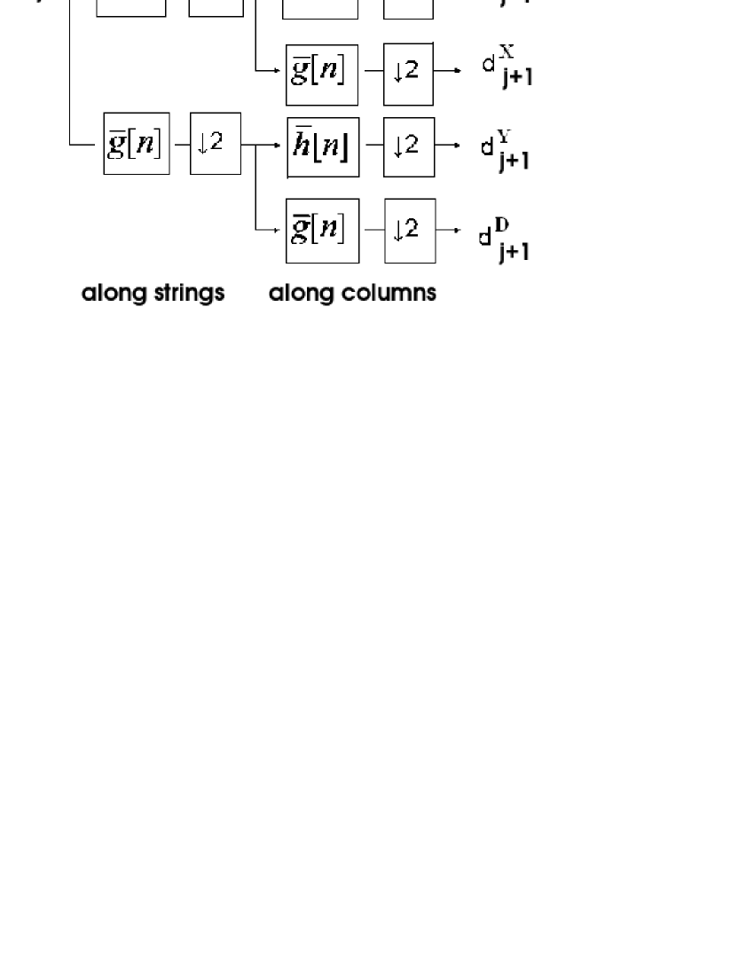
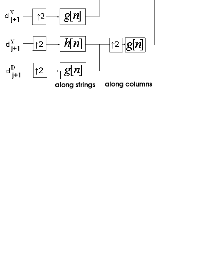
a)                                                             b)

Figure 1: Symbolic schemes of the two-dimensional DWT: a) decomposition and b) restoration

Wavelet analysis of complex structures in two-dimensional distributions

The wavelet analysis is often called a mathematical microscope since it allows to examine a signal with different resolution and to reveal structures on different scales. We demonstrate it here with some examples using Daubechies wavelet $D^{8}$ ten_lect . DWT with Daubechies $D^{8}$ was tested by the example of the one-dimensional function in vlk .

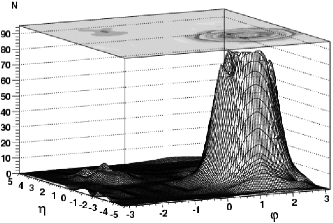
c)

Figure 2: Ring-like and jet-like structures in angular particle distribution: a) both structures, b) wavelet restoration without large scale coefficients, $d_{j}[n_{1},n_{2}]=0$ at $j=3,...,7$, c) wavelet restoration without small scale coefficients, $d_{j}[n_{1},n_{2}]=0$ at $j=1,...,3$. View in the upper plane of figures is the distribution projected on the plane.

In figure (fig.2a) the two-dimensional histogram of angular distribution in $\eta\times\varphi$ space is simulated from $N=100000$ entries, including the jet and ring-like shape as a toy example. The histogram binning is $128\times 128$. The values in each bin of the histogram determine the coefficients $a_{j=0}[n_{1},n_{2}]$ for the smallest scale $j=0$. The whole interval of the histogram along both axes $\eta$ and $\varphi$ corresponds to the scale $j=7$.

With the help of the wavelet analysis we try to reveal different forms of irregularities in the histogram. For this purpose we use the wavelet decomposition of the histogram and then restore its structure at different scales. If during restoration we set to zero the coefficients $d_{j}[n_{1},n_{2}]=0$ for large scales $j=3,4,5,6,7$, then only a narrow peak is restored (fig. 2b). If during restoration we set to zero the coefficients $d_{j}[n_{1},n_{2}]=0$ for small scales $j=1,2,3$ then the ring-like structure, which initially is present in the distribution, is revealed and the narrow peak disappears (fig. 2c).

Now we consider another example of the function containing two peaks of different shapes:

$$f(\eta,\varphi) = \frac{1}{\sqrt{(\eta-\eta_{0})^{2}+(\varphi-\varphi_{0})^{2}}}+$$ (5)

$$+ A\exp\{-0.5\frac{(\eta-\eta_{1})^{2}+(\varphi-\varphi_{1})^{2}}{\sigma^{2}}\}.$$

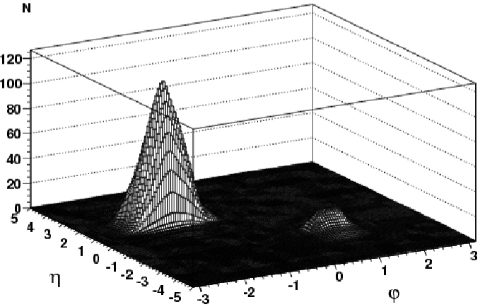
c)

Figure 3: Narrow and wide jets in angular particle distribution (5): a) both jets, b) wavelet restoration without large scale coefficients, $d_{j}[n_{1},n_{2}]=0$ at $j=3,...,7$, c) wavelet restoration without small scale coefficients, $d_{j}[n_{1},n_{2}]=0$ at $j=1,...,3$.

The chosen parameters are $~{}\sigma=0.4$ and $A=40$ (the particular values for peak positions are irrelevant and chosen for peaks not to overlap). The peaks have different widths. Therefore they correspond to different scales in wavelet expansion. Just as in the previous example, we produce the histogram from this function (fig. 3a). If we leave only coefficients $d_{j}[n_{1},n_{2}]$ for $j=1,2$ at small scales, we get the narrow peak (fig. 3b). The wide peak is restored quite well if in the wavelet series we leave coefficients $d_{j}[n_{1},n_{2}]$ at large scales $j=4,5,6$ (fig.3c).

Wavelet analysis of jet events

Jets of hadrons are usually well collimated along the jet axis, so we search by wavelet method for narrow peaks in the distribution of the transverse momentum $\frac{d^{2}p_{T}}{d\varphi d\eta}$. Jets with different transverse momenta $p_{T}$ were simulated for pp collisions at LHC energy $\sqrt{s}=5500$ GeV by PYTHIA event generator pythia . Then the angular distribution of particle transverse momentum was superimposed on the background, simulated by HYDJET generator lokhtin . The background is a sum of 100 events of PbPb collisions with multiplicity in the central rapidity region $(dN/dy)_{y=0}\approx 4000$. The jet production is switched off in the background events.

Histograms are made by binning of the two-dimensional distribution within intervals $|\eta|<2.4$ and $|\varphi|<\pi$ with the number of bins 128 for each variable. The sizes of bins are equal to $\Delta\eta\times\Delta\varphi=0.0375\times 0.049$ , which are close to CMS detector granularities. The wavelet analysis is used to find the position of jets. The background is treated as the large-scale structure (in our case $j=2-7$).

The following algorithm of jet recognition with the help of wavelet analysis is proposed:

1. A given event distribution is decomposed by the wavelet discrete transformation.

2. A smooth background at the large scale $j=7$ is evaluated and then subtracted from the distribution.

3. To remove the irregularities at the large scales the coefficients $d_{j}[n_{1},n_{2}],~{}j=4-7$ are set to zero. The range of small scales $j<4$ corresponds approximately to the region $\sqrt{(\bigtriangleup\eta)^{2}+(\bigtriangleup\varphi)^{2}}<R_{jet}=0.3$ from the center of the narrow peak.

4. The coefficients at small scales $d_{j}[n_{1},n_{2}],j=1,2,3$, which are below a certain threshold, are set to zero in order to remove the sharp irregularities with small intensity. These cuts correspond to conditions $d_{j}[n_{1},n_{2}]<cut\times(d_{j}[n_{1},n_{2}])_{max}$. The parameter $cut=0.95$ was found as optimum.

5. The event distribution is restored with the selected $d_{j}[n_{1},n_{2}]$ coefficients.

The event with three jets with total $p_{T}=53$ GeV, $p_{T}=45$ GeV and $p_{T}=22$ GeV in their regions is shown in fig.4 before background was added. The sum with background is shown in fig.5 . The same event with jet reconstruction by the proposed method is shown in fig. 6. Here the smooth background has been removed by setting to zero $d_{j}[n_{1},n_{2}]$ at largest scale $j=7$. The sharp peaks with small intensity in the background are removed by the cuts of small scale $d_{j}[n_{1},n_{2}]$-coefficients below the threshold. Position of jets is well allocated on position of peaks in the spectrum of wavelet coefficients at different scales depending on the width of a jet. Fig. 6 shows that the peak intensities are decreased and their shapes are distorted.

Only two jets are restored in this case. The third jet with $p_{T}=22$ GeV/c is lost because it is compatible to background fluctuations. Another disadvantage of this selection is very strong distortion of the total transverse momentum values. The calculation of jet energy must be made by other methods (for example, by the cone method). But the jet positions are reconstructed quite well by DWT.

The background under jet may be different and depend on jet position in $\eta-\varphi$ plane. So it is not correct to subtract background, calculated as average background in $\eta-\varphi$ space. Here we propose to estimate the background contribution under jet by calculating it inside a ring around the jet. Let we know a position of jet by wavelet analysis and select some region of jet as $\sqrt{(\bigtriangleup\eta)^{2}+(\bigtriangleup\varphi)^{2}}<R_{jet}$ . Then we can calculate the total transverse momentum in the ring $R_{jet}<\sqrt{(\bigtriangleup\eta)^{2}+(\bigtriangleup\varphi)^{2}}<R_{ring}$. In our case we take $R_{ring}$ so that the number of bins under jet and in the ring are equal.

Let’s define the average transverse momentum $<p_{T}>=\frac{1}{N{bin}}~{}\sum_{k=1}^{N{bin}}p_{T,k}$, where $N_{bin}$ is the number of bins in the region of jet or ring in angular distribution. The first (53 GeV/c) and second (45 GeV/c) jets have the average $<p_{T}>$ equal to $<p_{T}>_{jet}=0.346$ GeV/c and $0.295$ GeV/c. They are larger then those for background $<p_{T}>_{back}=0.330$ GeV/c and $0.246$ GeV/c. For the third jet (22 GeV/c) in Fig.6 the average $<p_{T}>_{jet}=0.143$ GeV/c is less then for background ($<p_{T}>_{back}=0.209$ GeV/c). Thus the wavelet analysis can’t find this jet.

The best way to study jet events with large background by wavelet method is as follows. First, one finds positions of jets by suggested procedure. Then the background contribution is calculated in the ring region around each jet. The genuine energy of the jet is obtained by the subtraction of the background contribution from the total energy in the jet region.

a)

b)

Conclusions

Wavelet analysis allows to find jets and ring-like structures in individual high multiplicity events in nucleus-nucleus collisions. The two-dimensional discrete wavelet transformation reveals well the irregularities with different shapes by corresponding choice of the wavelet scale $j$. Such structures correspond to different effects in nucleus-nucleus collisions. The ring-like structure is impossible to reveal by well known jet algorithms, but this goal is achieved with the help of the wavelet analysis. The method is applied to the jet-like event with high multiplicity background for the first time. The DWT allows also to distinguish the bumps with different widths in two-dimensional angular distribution in the same event. It is very important for diagnostics of quark and qluon jets.

a)

b)

Discrete wavelet transformation was tested on the particle angular distributions, which are close to foreseen experimental LHC data. Position of jets is well allocated on position of peaks in the spectrum of wavelet coefficients at different scales depending on the width of a jet. Removing the wavelet coefficients at large scales allows to substract the smooth background. Removing the wavelet coefficients at small scales below certain threshold allows ”to clean out” event from the sharp irregularities with small intensity.

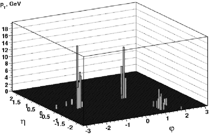
Figure 4: The event with jet transverse momenta $p_{T}=53$ GeV, $p_{T}=45$ GeV and $p_{T}=22$ GeV, simulated by PYTHIA.

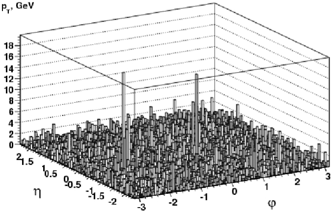
Figure 5: Sum of the event and the background, calculated by HYDJET.

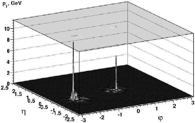
Figure 6: The distribution of the event (see Fig.4) after restoration by suggested method of jet searching.

One must be careful with excluding the background by wavelet analysis. Its subtraction can decrease the jet intensity (energy, number of particles) and change the jet shape. It can be recommended for use only to find the jet position. The jet energy must be estimated by other methods. However, the jet position is defined quite well by the discrete wavelet transformation.

At the end we would like to stress that the wavelet analysis can be used more widely for studies of the general topology of individual high multiplicity events. Beside jets and rings, other structures of mini-bias events can be found as was noted already. Common features of correlations in particle locations within the three-dimensional phase space such as fractality and intermittency can be revealed ddk .

References

- (1) I. Arsene et al. (BRAHMS), Nucl. Phys. A757 (2005) 1, nucl-ex/0410020.
- (2) B. Back et al. (PHOBOS), Nucl. Phys. A757 (2005) 28, nucl-ex/050641.
- (3) J. Adams et al. (STAR), Nucl. Phys. A757 (2005) 102, nucl-ex/0501009.
- (4) K. Adcox et al. (PHENIX), Nucl. Phys. A757 (2005) 184, nucl-ex/0410003
- (5) I.N. Vardanyan et al., Phys. Atom. Nucl. 68 (2005) 302.
- (6) A.V. Apanasenko et al., JETP Lett. 30 (1979) 145.
- (7) I.M. Dremin et al., Phys. Lett. B499 (2001) 97.
- (8) N.N. Ajitanand (PHENIX), nucl-ex/0609038.
- (9) I.M. Dremin, JETP Lett. 30 (1979) 140; Sov. J. Nucl Phys. 33 (1981) 726.
- (10) I.M. Dremin, Nucl. Phys. A767 (2006) 233.
- (11) I.M. Dremin, Int. J. Mod. Phys. A22 (2007) 3087.
- (12) H. Stöcker et al., Prog. Part. Nucl. Phys. 4 (1980) 133.
- (13) H. Stöcker, Nucl. Phys. 750 (2005) 123.
- (14) J. Casalderrey-Solana et al., Nucl. Phys. A774 (2006) 577.
- (15) C. Albajar et al., Nucl. Phys. B309 (1988) 405.
- (16) J. Adams et al., arXiv:nucl-ex/0407001, arXiv:0706.0596.
- (17) G. Georgopoulos et al., Mod. Phys. Lett. A15 (2000) 1051.
- (18) V. de la Mota1, F. Sa bille, Acta Physica Hungarica, A) Heavy Ion Physics 16 (2002) 203.
- (19) N.M. Astafyeva et al., Mod. Phys. Lett. A12 (1997) 1185.
- (20) V.V. Uzhinskii et al., hep-ex/0206003 (2002).
- (21) I. Berden et al., Phys. Rev. C65 (2002) 044903.
- (22) M. Kopytine, arXiv:nucl-ex/0211015 (2002).
- (23) G. Arnison et al., (UA1), Phys. Lett. B123 (1983) 115.
- (24) I.P. Lokhtin, A.M. Snigirev, Eur. Phys. J. C45 (2006) 211.
- (25) M. Bedjidian et al., CMS Notes 1996/016.
- (26) T. Sjöstrand et al., Comput. Phys. Commun., 135:238, 2001. [arXiv:hep-ph/0010017].
- (27) C. Mallat, ”A wavelet tour of signal processing”, Academic Press, 1999.
- (28) I. Daubeuchies, “Ten lectures on wavelets”, Soc. for Industrial and Applied Mathematics, Philadelphia, Pennsylvania, 1992.
- (29) I.M. Dremin et al., Physics-Uspekhi 42 (2001) 447, hep-ph/0101182.
- (30) V.L. Korotkikh, Preprint SINP MSU-2002-6/690 (2000).
- (31) E.A. DeWolf et al., Phys. Rep. 270 (1996) 1.