The Symplectic Geometry of Penrose Rhombus Tilings

Abstract

The purpose of this article is to view Penrose rhombus tilings from the perspective of symplectic geometry. We show that each thick rhombus in such a tiling can be naturally associated to a highly singular $4$–dimensional compact symplectic space $M_{R}$, while each thin rhombus can be associated to another such space $M_{r}$; both spaces are invariant under the Hamiltonian action of a $2$–dimensional quasitorus, and the images of the corresponding moment mappings give the rhombuses back. The spaces $M_{R}$ and $M_{r}$ are diffeomorphic but not symplectomorphic.

Mathematics Subject Classification. Primary: 53D20. Secondary: 52C23

Introduction

We start by considering a Penrose tiling by thick and thin rhombuses (cf. [11]). Rhombuses are very special examples of simple convex polytopes. Because of the Atiyah, Guillemin–Sternberg convexity theorem [1, 8], convex polytopes can arise as images of the moment mapping for Hamiltonian torus actions on compact symplectic manifolds. For example, simple convex polytopes that are rational with respect to a lattice $L$ and satisfy an additional integrality condition, correspond to symplectic toric manifolds. More precisely, the Delzant theorem [6] tells us that to each such polytope in $(\mbox{\bbb{R}}^{n})^{*}$, there corresponds a compact symplectic $2n$–dimensional manifold $M$, endowed with the effective Hamiltonian action of a torus of dimension $n$. As it turns out, the polytope is exactly the image of the corresponding moment mapping. One of the striking features of Delzant’s theorem is that it gives an explicit procedure to obtain the manifold corresponding to each given polytope as a symplectic reduced space. This correspondence may be applied to each of the rhombuses in a Penrose tiling separately. However, the rhombuses in a Penrose tiling, though simple and convex, are not simultaneously rational with respect to the same lattice. Therefore we cannot apply the Delzant procedure simultaneously to all rhombuses in the tiling. However, if we replace the lattice with a quasilattice (the ℤ–span of a set of ℝ–spanning vectors) and the manifold with a suitably singular space, then it is possible to apply a generalization of the Delzant procedure to arbitrary simple convex polytopes that was given by the second named author in [14]. According to this result, to each simple convex polytope in $(\mbox{\bbb{R}}^{n})^{*}$, and to each suitably chosen quasilattice $Q$, one can associate a family of compact symplectic $2n$–dimensional quasifolds $M$, each endowed with the effective Hamiltonian action of the quasitorus $(\mbox{\bbb{R}}^{n})^{*}/Q$, having the property that the image of the corresponding moment mapping is the polytope itself. Quasifolds are generalizations of manifolds and orbifolds that were introduced in [14]. A local model for a $k$–dimensional quasifold is given by the topological quotient of an open subset of $\mbox{\bbb{R}}^{k}$ by the action of a finitely generated group. A $k$–dimensional quasifold is a topological space admitting an atlas of $k$–dimensional local models that are suitably glued together. It is a highly singular, usually not even Hausdorff, space. A quasitorus is the natural generalization of a torus in this setting.

We remark that, unlike the Delzant case, we do not have here a one–to–one correspondence between polytopes and symplectic spaces. In fact, there is much more freedom of choice in the generalized Delzant construction, and infinitely many symplectic quasifolds will map to the same polytope. More precisely, given any suitable quasilattice $Q$, the construction will yield one quasifold for each choice of a set of vectors $X_{1},\ldots,X_{d}$ in $Q$, each of which is orthogonal and pointing inwards to one of the $d$ different facets of the polytope. The striking fact in the case of a Penrose tiling is that there is a natural choice of a quasilattice and of a set of inward–pointing vectors, and therefore a natural choice of a privileged quasifold mapping to each tile. In fact, let us consider a Penrose rhombus tiling where all rhombuses have edges of length $1$; we will see in Section 1 that such a tiling determines a star of five unit vectors, pointing to the vertices of a regular pentagon. One of the features of the tiling is that the four edges of any given rhombus in the tiling are orthogonal to two of these five vectors. These two vectors, and their opposites, will be our natural choice of the four inward–pointing vectors in the Delzant construction. The span over the integers of the five vectors in the star is dense in $\mbox{\bbb{R}}^{2}$, this is the quasilattice that is associated to the tiling, and will be our choice of quasilattice.

Moreover, we show that all the different rhombuses yield only two possible compact symplectic quasifolds: one for all the thick rhombuses, $M_{R}$, and one for all the thin ones, $M_{r}$. Both are global quotients of a product of two spheres modulo the action of a finitely generated group; they are diffeomorphic, but not symplectomorphic. Notice that in general a quasifold is not a global quotient of a manifold modulo the action of a finitely generated group, in fact most of the examples are not, see the examples worked out in [14] and the quasifold corresponding to the Penrose kite in [4].

We remark that quasilattices are quasiperiodic structures underlying quasiperiodic tilings and the atomic order of quasicrystals, which were discovered in the eighties by observing that the diffraction pattern of such materials is not periodic, but quasiperiodic, with 5–fold rotational symmetries (cf. [17]). In forthcoming work [5] we give a symplectic interpretation of three–dimensional analogues of Penrose tilings, that represent structure models for icosahedral quasicrystals.

The paper is structured as follows. In the first section we recall some basic facts on Penrose rhombus tilings. In the second section we recall from [14] the notions of symplectic quasifold, of quasitorus actions, and the generalization of the Delzant procedure. In the third section we apply all of the above to construct the quasifolds $M_{R}$ and $M_{r}$, from special choices of one thick rhombus and of one thin rhombus in a given Penrose tiling. Finally in the fourth section we show that all the other thick rhombuses of the tiling correspond to $M_{R}$, that all the other thin rhombuses correspond to $M_{r}$ and that $M_{R}$ and $M_{r}$ are diffeomorphic but not symplectomorphic.

1 Penrose Rhombus Tilings

1.1 Penrose Rhombuses

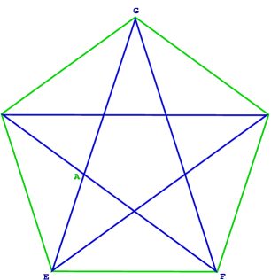
Figure 1: The pentagram

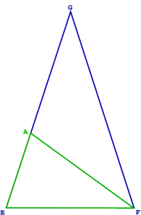
Figure 2: The golden triangle and its decomposition

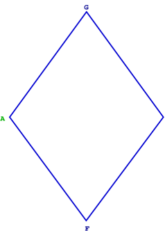
Figure 3: The thick rhombus

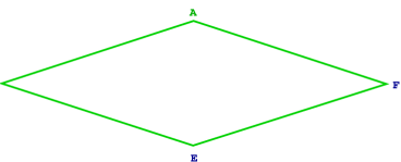
Figure 4: The thin rhombus

Let us now recall the procedure for obtaining the Penrose rhombuses from the pentagram. For a proof of the facts that are needed we refer the reader to [10], and for additional historical remarks we refer the reader to [15]. Let us consider a regular pentagon whose edges have length one and let us consider the corresponding inscribed pentagram, as in Figure 1. It can be shown that the ratio of the diagonal to the side of the pentagon is equal to the golden ratio, $\phi=\frac{1+\sqrt{5}}{2}=2\cos{\frac{\pi}{5}}$. Therefore the triangle having vertices E, F, G is a golden triangle, which is, by definition, an isosceles triangle with a ratio of side to base given by $\phi$. This triangle decomposes into the two smaller triangles of vertices E, F, A and F, G, A, respectively (see Figure 2). The first one is itself a golden triangle. Using the fundamental relation

$$\phi=1+\frac{1}{\phi}$$ (1)

one can show that the second one is a golden gnomon, which is, by definition, an isosceles triangle with a ratio of side to base given by $\frac{1}{\phi}$. Now, if we consider the union of the golden gnomon with its reflection with respect to the FG–axis, we obtain the thick rhombus (see Figure 3), while to obtain the thin rhombus we consider the union of the smaller golden triangle with its reflection with respect to the EG–axis (see Figure 4). Notice that the angles of the thick rhombus measure $2\pi/5$ and $3\pi/5$, while the angles of the thin rhombus measure $\pi/5$ and $4\pi/5$.

1.2 The Tiling Construction

We now briefly recall some basic facts about Penrose rhombus tilings; for a deeper analysis of this important subject we refer the reader to the original paper by Penrose [11], to his subsequent works [12, 13], to Austin’s articles [2, 3] and finally, for a review, to the books by Grünbaum and Shephard [7] and by Senechal [16]. We start with the following

Definition 1.1 (Penrose rhombus tiling)

A Penrose rhombus tiling is a tiling of the plane by thick and thin rhombuses that obey the matching rules shown in Figures 5 and 6.

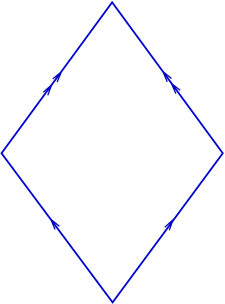
Figure 5: Matching rules for the thick rhombus

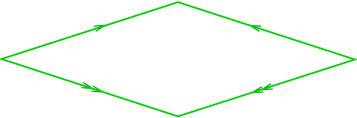
Figure 6: Matching rules for the thin rhombus

Consider a Penrose tiling in $(\mbox{\bbb{R}}^{2})^{*}$ with rhombuses having edges of length $1$ (Figure 7);

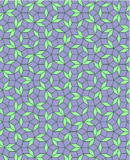
Figure 7: A Penrose rhombus tiling. Figure by D. Austin [2], reprinted courtesy of the AMS

it is well–known that there are uncountably many such tilings and that each of them is non periodic. The key remark in our set–up is that there exist a quasilattice, and a set of vectors contained in it, that are naturally associated to any such tiling. First of all we need to give the formal definition of quasilattice:

Definition 1.2 (Quasilattice)

Let $V$ be a real vector space. A quasilattice in $V$ is the Span over ℤ of a set of ℝ–spanning vectors $V_{1},\ldots,V_{d}$ of $V$.

Notice that $\hbox{Span}_{\mbox{\bbb{Z}}}\{V_{1},\dots,V_{d}\}$ is a lattice if and only if it admits a set of generators which is a basis of $V$. Consider now, in $(\mbox{\bbb{R}}^{2})^{*}$, the star ${\mathcal{S}}^{*}$ of five unit vectors

$$\left\{\begin{array}[]{l}Y^{*}_{0}=(0,1)\\ Y^{*}_{1}=\frac{1}{2}(-\sqrt{2+\phi},\frac{1}{\phi})\\ Y^{*}_{2}=\frac{1}{2}(-\frac{1}{\phi}\sqrt{2+\phi},-\phi,)\\ Y^{*}_{3}=\frac{1}{2}(\frac{1}{\phi}\sqrt{2+\phi},-\phi)\\ Y^{*}_{4}=\frac{1}{2}(\sqrt{2+\phi},\frac{1}{\phi})\end{array}\right.$$

Figure 8: Dual star ${\mathcal{S}}^{*}$

Let $R$ be the quasilattice generated by the vectors of ${\mathcal{S}}^{*}$, namely

$$R=\hbox{Span}_{\mbox{\bbb{Z}}}\{Y^{*}_{0},\dots,Y^{*}_{4}\}.$$

The quasilattice $R$ is not a lattice, it is dense in $\mbox{\bbb{R}}^{2}$ and a minimal set of generators of $R$ is made of $4$ vectors. The following statement describes the relationship between the Penrose rhombus tilings considered and the quasilattice $R$, together with its generators.

Let us consider the five thick rhombuses that are determined by $Y_{k}^{*},Y_{k+1}^{*}$, for $k=0,\dots,4$, we denote them by $\Delta_{R}^{k}$, and the five thin rhombuses that are determined by $Y_{k}^{*},Y^{*}_{k+2}$, for $k=0,\dots,4$, we denote them by $\Delta_{r}^{k}$ (we are assuming here $Y^{*}_{5}=Y^{*}_{0}$ and $Y^{*}_{6}=Y^{*}_{1}$).

Let us consider any Penrose rhombus tiling $\mathcal{T}$ with rhombuses having edges of length $1$ and denote one of its edges by $AB$. From now on we will choose our coordinates so that $A=O$ and $B-A=Y^{*}_{0}$.

Proposition 1.3

Let $\mathcal{T}$ be a Penrose rhombus tiling with rhombuses having edges of length $1$. Then each rhombus is the translate of either a thick rhombus $\Delta_{R}^{k}$, $k=0,\ldots,4$, or of a thin rhombus $\Delta_{r}^{k}$, $k=0,\ldots,4$. Moreover each vertex of the tiling lies in the quasilattice $R$.

Proof.  The argument is very simple. Let $C$ be a vertex of the tiling that is different from $0$ and the above vertex $B$. We can walk from $B$ to $C$ on a path made of subsequent edges of the tiling. We denote the vertices of the broken line thus obtained by $T_{0}=A,T_{1}=B,\dots,T_{j},\dots,T_{m}=C$. The angle of the broken line at each vertex $T_{j}$ is necessarily a multiple of $\pi/5$. Therefore each vector $V_{j}=T_{j}-T_{j-1}$ is one of the vectors $\pm Y^{*}_{k}$, $k=0,\ldots,4$. Since $C-A=T_{m}-T_{0}=V_{m}+\cdots+V_{1}$ the vertex $C$ lies in $R$ and each rhombus having $C$ as vertex has edges parallel to two vectors of $S^{*}$. $\sqcap$$\sqcup$

Consider now the star of vectors $\mathcal{S}$ in $\mbox{\bbb{R}}^{2}$ given by:

$$\left\{\begin{array}[]{l}Y_{0}=(1,0)\\ Y_{1}=(\cos{\frac{2\pi}{5}},\sin{\frac{2\pi}{5}})=\frac{1}{2}(\frac{1}{\phi},\sqrt{2+\phi})\\ Y_{2}=(\cos{\frac{4\pi}{5}},\sin{\frac{4\pi}{5}})=\frac{1}{2}(-\phi,\frac{1}{\phi}\sqrt{2+\phi})\\ Y_{3}=(\cos{\frac{6\pi}{5}},\sin{\frac{6\pi}{5}})=\frac{1}{2}(-\phi,-\frac{1}{\phi}\sqrt{2+\phi})\\ Y_{4}=(\cos{\frac{8\pi}{5}},\sin{\frac{8\pi}{5}})=\frac{1}{2}(\frac{1}{\phi},-\sqrt{2+\phi})\end{array}\right.$$ (2)

Figure 9: Star $\mathcal{S}$

It is easy to check that for each $k$ the four vectors $\pm Y_{k},\pm Y_{k+1}$ are each orthogonal and inward–pointing to one of the different edges of the thick rhombus $\Delta_{R}^{k}$. In the same way the four vectors $\pm Y_{k},\pm Y_{k+2}$ are each orthogonal and inward–pointing to one of the different edges of the thin rhombus $\Delta_{r}^{k}$. By Proposition 1.3, the same is true for each thick and thin rhombus of any given tiling.

We denote by $Q$ the quasilattice generated by the vectors of $S$, namely

$$Q=\hbox{Span}_{\mbox{\bbb{Z}}}\{Y_{0},\dots,Y_{4}\}.$$ (3)

The following relations are necessary for determining the groups involved in the construction of the quasifolds corresponding to the rhombuses. If we write each $Y_{k}$, in complex notation, as $Y_{k}=e^{\frac{2k\pi i}{5}}$, then it can be easily verified that

$$\begin{array}[]{l}Y_{k+2}=-Y_{k}+\frac{1}{\phi}Y_{k+1}\\ Y_{k+4}=\frac{1}{\phi}Y_{k}-Y_{k+1}\\ \end{array}$$ (4)

and

$$\begin{array}[]{l}Y_{k+3}=-Y_{k+2}-\phi Y_{k}\\ Y_{k+4}=-\phi Y_{k+2}-Y_{k}.\\ \end{array}$$ (5)

Moreover $Y_{0}=-(Y_{1}+Y_{2}+Y_{3}+Y_{4})$ and $\{Y_{1},Y_{2},Y_{3},Y_{4}\}$ is a minimal set of generators of $Q$.

2 Symplectic Quasifolds

Let us recall the definition of quasifold; we refer to the article [14] for the missing details and proofs. We begin by defining the

Definition 2.1 (Quasifold model)

Let $\tilde{V}$ be a connected open subset of $\mbox{\bbb{R}}^{k}$ and let $\Gamma$ be a finitely generated group acting smoothly on $\tilde{V}$ so that the set of points, $\tilde{V}_{0}$, where the action is free, is connected and dense. Consider the space of orbits, $\tilde{V}/\Gamma$, of the action of the group $\Gamma$ on $\tilde{V}$, endowed with the quotient topology, and the canonical projection $p\;\colon\;\tilde{V}\rightarrow\tilde{V}/\Gamma$. A quasifold model of dimension $k$ is the triple $(\tilde{V}/\Gamma,p,\tilde{V})$, shortly denoted $\tilde{V}/\Gamma$.

Definition 2.2 (Submodel)

Consider a model $(\tilde{V}/\Gamma,p,\tilde{V})$ and let $W$ be an open subset of $\tilde{V}/\Gamma$. We will say that $W$ is a submodel of $(\tilde{V}/\Gamma,p,\tilde{V})$, if $(W,p,p^{-1}(W))$ defines a model.

Remark 2.3

Consider a model of dimension $k$, $(\tilde{V}/\Gamma,p,\tilde{V})$, such that there exists a covering $\pi\,\colon\,V^{\sharp}\rightarrow\tilde{V}$, where $V^{\sharp}$ is an open subset of $\mbox{\bbb{R}}^{k}$ acted on by a finitely generated group $\Pi$ in a smooth, free and proper fashion with $\tilde{V}=V^{\sharp}/\Pi$. Consider the extension of the group $\Gamma$ by the group $\Pi$

$$1\longrightarrow\Pi\longrightarrow\Gamma^{\sharp}\longrightarrow\Gamma\longrightarrow 1$$

defined as follows

$$\Gamma^{\sharp}=\left\{\;\gamma^{\sharp}\in\mbox{Diff}(V^{\sharp})\;|\;\exists\;\gamma\in\Gamma\;\mbox{s. t.}\;\pi(\gamma^{\sharp}(u^{\sharp}))=\gamma\circ\pi(u^{\sharp})\;\forall\;u^{\sharp}\in V^{\sharp}\;\right\}.$$

It is easy to verify that $\Gamma^{\sharp}$ is finitely generated, that it acts on $V^{\sharp}$ according to the assumptions of Definition 2.1 and that $\tilde{V}/\Gamma=V^{\sharp}/\Gamma^{\sharp}$. Let $p^{\sharp}=p\circ\pi$, we will then say that the model $(V^{\sharp}/\Gamma^{\sharp},p^{\sharp},V^{\sharp})$ is a covering of the model $(\tilde{V}/\Gamma,p,\tilde{V})$.

Definition 2.4 (Smooth mapping, diffeomorphism of models)

Given two models $(\tilde{V}/\Gamma,p,\tilde{V})$ and $(\tilde{W}/\Delta,q,\tilde{W})$, a mapping $f\,\colon\,\tilde{V}/\Gamma\longrightarrow\tilde{W}/\Delta$ is said to be smooth if there exist coverings in the sense of Remark 2.3 of the two given models, $(V^{\sharp}/\Gamma^{\sharp},p^{\sharp},V^{\sharp})$ and $(W^{\sharp}/\Delta^{\sharp},q^{\sharp},W^{\sharp})$, and a smooth mapping $f^{\sharp}\,\colon\,V^{\sharp}\longrightarrow W^{\sharp}$ such that $q^{\sharp}\circ f^{\sharp}=f\circ p^{\sharp}$; we will then say that $f^{\sharp}$ is a lift of $f$. We will say that the smooth mapping $f$ is a diffeomorphism of models if it is bijective and if the lift $f^{\sharp}$ is a diffeomorphism.

If the mapping $f^{\sharp}$ is a lift of a smooth mapping of models $f\,\colon\,\tilde{U}/\Gamma\longrightarrow\tilde{V}/\Delta$ so are the mappings ${f^{\sharp}}^{\gamma}(-)=f^{\sharp}(\gamma\cdot-)$, for all elements $\gamma$ in $\Gamma^{\sharp}$ and ${}^{\delta}f^{\sharp}(-)=\delta\cdot f^{\sharp}(-)$, for all elements $\delta$ in $\Delta^{\sharp}$. We recall that if the mapping $f$ is a diffeomorphism, then these are the only other possible lifts:

Lemma 2.5

Consider two models, $\tilde{U}/\Gamma$ and $\tilde{V}/\Delta$, and let $f\,\colon\,\tilde{U}/\Gamma\longrightarrow\tilde{V}/\Delta$ be a diffeomorphism of models. For any two lifts, $f^{\sharp}$ and $\bar{f}$, of the diffeomorphism $f$, there exists a unique element $\delta$ in $\Delta^{\sharp}$ such that $\bar{f}={}^{\delta}f^{\sharp}$.

Lemma 2.6

Consider two models, $\tilde{U}/\Gamma$ and $\tilde{V}/\Delta$, and a diffeomorphism $f\,\colon\,\tilde{U}/\Gamma\longrightarrow\tilde{V}/\Delta$. Then, for a given lift, $f^{\sharp}$, of the diffeomorphism $f$, there exists a group isomorphism $F\,\colon\,\Gamma^{\sharp}\longrightarrow\Delta^{\sharp}$ such that ${f^{\sharp}}^{\gamma}={}^{F(\gamma)}f^{\sharp}$, for all elements $\gamma$ in $\Gamma^{\sharp}$.

Similarly to the notion of smooth mapping it is possible to define other geometric objects on models, such as differential forms, symplectic forms and vector fields.

Definition 2.7 (Quasifold)

A dimension $k$ quasifold structure on a topological space $M$ is the assignment of an atlas, or collection of charts, ${\mathcal{A}}=\{\,(V_{\alpha},\tau_{\alpha},\tilde{V}_{\alpha}/\Gamma_{\alpha})\,|\,\alpha\in A\,\}$ having the following properties:

1. The collection $\{\,V_{\alpha}\,|\,\alpha\in A\,\}$ is a cover of $M$.

2. For each index $\alpha$ in $A$, the set $V_{\alpha}$ is open, the space $\tilde{V}_{\alpha}/\Gamma_{\alpha}$ defines a model, and the mapping $\tau_{\alpha}$ is a homeomorphism of the space $\tilde{V}_{\alpha}/\Gamma_{\alpha}$ onto the set $V_{\alpha}$.

3. For all indices $\alpha,\beta$ in $A$ such that $V_{\alpha}\cap V_{\beta}\neq\emptyset$, the sets $\tau_{\alpha}^{-1}(V_{\alpha}\cap V_{\beta})$ and $\tau_{\beta}^{-1}(V_{\alpha}\cap V_{\beta})$ are submodels of $\tilde{V}_{\alpha}/\Gamma_{\alpha}$ and $\tilde{V}_{\beta}/\Gamma_{\beta}$ respectively and the mapping

   $$g_{\alpha\beta}=\tau_{\beta}^{-1}\circ\tau_{\alpha}\,\colon\tau_{\alpha}^{-1}(V_{\alpha}\cap V_{\beta})\longrightarrow\tau_{\beta}^{-1}(V_{\alpha}\cap V_{\beta})$$

   is a diffeomorphism of models. We will then say that the mapping $g_{\alpha\beta}$ is a change of charts and that the corresponding charts are compatible.

4. The atlas $\mathcal{A}$ is maximal, that is: if the triple $(V,\tau,\tilde{V}/\Gamma)$ satisfies property 2. and is compatible with all the charts in $\mathcal{A}$, then $(V,\tau,\tilde{V}/\Gamma)$ belongs to $\mathcal{A}$.

We will say that a space $M$ with a quasifold structure is a quasifold.

Remark 2.8

Remark that, by the definition of diffeomorphism, finitely generated groups corresponding to different charts need not be isomorphic (see the fundamental example of the quasisphere in [14]).

Remark 2.9

To each point $m\in M$ there corresponds a finitely generated group $\Gamma_{m}$ defined as follows: take a chart $(V_{\alpha},\tau_{\alpha},\tilde{V}_{\alpha}/\Gamma_{\alpha})$ around $m$, then $\Gamma_{m}$ is the isotropy group of $\Gamma_{\alpha}$ at any point $\tilde{v}\in\tilde{V}$ which projects down to $m$. One can check that this definition does not depend on the choice of the chart. If all the $\Gamma_{m}$’s are finite $M$ is an orbifold, if they are trivial then $M$ is a manifold.

It is possible to define on any quasifold $M$ the notions of smooth mapping, diffeomorphism, differential form, symplectic form and smooth vector field.

Definition 2.10 (Quasitorus)

A quasitorus of dimension $n$ is the quotient $\mbox{\bbb{R}}^{n}/Q$, where $Q$ is a quasilattice in $\mbox{\bbb{R}}^{n}$.

We remark that a quasitorus is an example of quasifold covered by one chart. At this point one can define the notion of Hamiltonian action of a quasitorus on a symplectic quasifold, and the corresponding moment mapping.

3 The Tiles from a Symplectic Viewpoint

We now outline the generalization of the Delzant procedure [6] to nonrational simple convex polytopes that is proven in [14]. We begin by recalling what is a

Definition 3.1 (Simple polytope)

A dimension $n$ convex polytope $\Delta\subset(\mbox{\bbb{R}}^{n})^{*}$ is said to be simple if there are exactly $n$ edges stemming from each vertex.

Let us now consider a dimension $n$ convex polytope $\Delta\subset(\mbox{\bbb{R}}^{n})^{*}$. If $d$ is the number of facets of $\Delta$, then there exist elements $X_{1},\ldots,X_{d}$ in $\mbox{\bbb{R}}^{n}$ and $\lambda_{1},\ldots,\lambda_{d}$ in ℝ such that

$$\Delta=\bigcap_{j=1}^{d}\{\;\mu\in(\mbox{\bbb{R}}^{n})^{*}\;|\;\langle\mu,X_{j}\rangle\geq\lambda_{j}\;\}.$$ (6)

Definition 3.2 ($Q$–rational polytope)

Let $Q$ be a quasilattice in $\mbox{\bbb{R}}^{n}$. A convex polytope $\Delta\subset(\mbox{\bbb{R}}^{n})^{*}$ is said to be $Q$–rational, if the vectors $X_{1},\ldots,X_{d}$ can be chosen in $Q$.

All polytopes in $(\mbox{\bbb{R}}^{n})^{*}$ are $Q$–rational with respect to some quasilattice $Q$; it is enough to consider the quasilattice that is generated by the elements $X_{1},\ldots,X_{d}$ in (6). Notice that if the quasilattice is a honest lattice then the polytope is rational.

In our situation we only need to consider the special case of simple convex polytopes in $2$–dimensional space. Let $Q$ be a quasilattice in $\mbox{\bbb{R}}^{2}$ and let $\Delta$ be a simple convex polytope in the space $(\mbox{\bbb{R}}^{2})^{*}$ that is $Q$–rational. Consider the space $\mbox{\bbb{C}}^{d}$ endowed with the standard symplectic form $\omega_{0}=\frac{1}{2\pi i}\sum_{j=1}^{d}dz_{j}\wedge d\bar{z}_{j}$ and the standard action of the torus $T^{d}=\mbox{\bbb{R}}^{d}/\mbox{\bbb{Z}}^{d}$:

$$\begin{array}[]{cccccl}\tau\,\colon&T^{d}&\times&\mbox{\bbb{C}}^{d}&\longrightarrow&\mbox{\bbb{C}}^{d}\\ &((e^{2\pi i\theta_{1}},\ldots,e^{2\pi i\theta_{d}})&,&\underline{z})&\longmapsto&(e^{2\pi i\theta_{1}}z_{1},\ldots,e^{2\pi i\theta_{d}}z_{d}).\end{array}$$

This action is effective and Hamiltonian and its moment mapping is given by

$$\begin{array}[]{cccl}J\,\colon&\mbox{\bbb{C}}^{d}&\longrightarrow&(\mbox{\bbb{R}}^{d})^{*}\\ &\underline{z}&\longmapsto&\sum_{j=1}^{d}|z_{j}|^{2}e_{j}^{*}+\lambda,\quad\lambda\in(\mbox{\bbb{R}}^{d})^{*}\;\mbox{constant}.\end{array}$$

The mapping $J$ is proper and its image is the cone ${\mathcal{C}}_{\lambda}=\lambda+{\mathcal{C}}_{0}$, where ${\mathcal{C}}_{0}$ denotes the positive orthant in the space $(\mbox{\bbb{R}}^{d})^{*}$. Now consider the surjective linear mapping

$$\pi\,\colon \mbox{\bbb{R}}^{d}\longrightarrow\mbox{\bbb{R}}^{2},$$

$$e_{j}\longmapsto X_{j}$$

and the dimension $2$ quasitorus $D=\mbox{\bbb{R}}^{2}/Q$. Then the linear mapping $\pi$ induces a quasitorus epimorphism $\Pi\,\colon\,T^{d}\longrightarrow D$. Define now $N$ to be the kernel of the mapping $\Pi$ and choose $\lambda=\sum_{j=1}^{d}\lambda_{j}e_{j}^{*}$. Denote by $i$ the Lie algebra inclusion $\mbox{\frak n}=\mbox{Lie}(N)\rightarrow\mbox{\bbb{R}}^{d}$ and notice that $\Psi=i^{*}\circ J$ is a moment mapping for the induced action of $N$ on $\mbox{\bbb{C}}^{d}$. Then the quasitorus $T^{d}/N$ acts in a Hamiltonian fashion on the compact symplectic quasifold $M=\Psi^{-1}(0)/N$. If we identify the quasitori $D$ and $T^{d}/N$ using the epimorphism $\Pi$, we get a Hamiltonian action of the quasitorus $D$ whose moment mapping has image equal to ${(\pi^{*})}^{-1}({\mathcal{C}}_{\lambda}\cap\ker{i^{*}})={(\pi^{*})}^{-1}({\mathcal{C}}_{\lambda}\cap\mbox{im}\,\pi^{*})={(\pi^{*})}^{-1}(\pi^{*}(\Delta))$ which is exactly $\Delta$. This action is effective since the level set $\Psi^{-1}(0)$ contains points of the form $\underline{z}\in\mbox{\bbb{C}}^{d}$, $z_{j}\neq 0$, $j=1,\ldots,d$, where the $T^{d}$–action is free. Notice finally that $\dim{M}=2d-2\dim{N}=2d-2(d-2)=4=2\dim{D}$. If we take $Q$ to be an ordinary lattice, the space $M$ is either a manifold or an orbifold, in accordance with the generalization of Delzant’s construction to arbitrary simple rational polytopes by Lerman and Tolman [9].

Let us remark that this construction depends on two arbitrary choices: the choice of the quasilattice $Q$ with respect to which the polytope is $Q$–rational, and the choice of the inward–pointing vectors $X_{1},\ldots,X_{d}$ in $Q$.

From now on we fix the quasilattice $Q$ that is generated by the vectors in the star ${\mathcal{S}}$ defined by (2). It follows from Subsection 1.2 that the rhombuses of any tiling are $Q$–rational with respect to $Q$, in our chosen coordinate system. The natural choices of inward–pointing vectors are given by $\pm Y_{k},\pm Y_{k+1}$ for $\Delta^{k}_{R}$, and by $\pm Y_{k},\pm Y_{k+2}$ for $\Delta_{r}^{k}$.

Let us begin by performing the generalized Delzant construction for the thick rhombus $\Delta_{R}^{2}$ and for the thin rhombus $\Delta_{r}^{4}$. We will show in Theorem 4.1 that all the other cases can be reduced to these two.

3.1 The Thick Rhombus

Let us consider the thick rhombus $\Delta_{R}^{2}$ and let us label its edges with the numbers $1,2,3,4$, as in Figure 10.

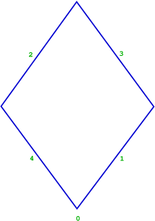
Figure 10: The thick rhombus $\Delta_{R}^{2}$

The corresponding inward–pointing vectors are given by $X_{1}=Y_{2}$, $X_{2}=-Y_{2}$, $X_{3}=Y_{3}$, $X_{4}=-Y_{3}$, while $\lambda_{1}=\lambda_{4}=0$, and $\lambda_{2}=\lambda_{3}=-\frac{1}{2}\sqrt{2+\phi}$. Let us consider the linear mapping defined by

$$\begin{array}[]{cccc}\pi\colon&\mbox{\bbb{R}}^{4}&\rightarrow&\mbox{\bbb{R}}^{2}\\ &e_{i}&\mapsto&X_{i}.\end{array}$$

Its kernel, n, is the $2$-dimensional subspace of $\mbox{\bbb{R}}^{4}$ that is spanned by $e_{1}+e_{2}$ and $e_{3}+e_{4}$. It is the Lie algebra of $N=\{\,\exp(X)\in T^{4}\,|\,X\in\mbox{\bbb{R}}^{4},\pi(X)\in Q\,\}$. If $\Psi$ is the moment mapping of the induced $N$–action, then

$$\Psi(z_{1},z_{2},z_{3},z_{4})=\left(|z_{1}|^{2}+|z_{2}|^{2}-\frac{1}{2}\sqrt{2+\phi},|z_{3}|^{2}+|z_{4}|^{2}-\frac{1}{2}\sqrt{2+\phi}\right).$$

Let $R=\left(\frac{1}{2}\sqrt{2+\phi}\right)^{1/2}$ and denote by $S^{3}_{R}$ and $S^{2}_{R}$ the spheres of radius $R$, centered at the origin, of dimension $3$ and $2$ respectively. Then $\Psi^{-1}(0)=S_{R}^{3}\times S_{R}^{3}$. A straightforward computation, using the relations (4), with $k=2$, gives that

$$N=\left\{\,\exp(X)\in T^{4}\,|\,X=\left(s,s+\frac{1}{\phi}h,t,t+\frac{1}{\phi}k\right),s,t\in\mbox{\bbb{R}},h,k\in\mbox{\bbb{Z}}\,\right\},$$

which, for equation (1), is equal to

$$\left\{\,\exp(X)\in T^{4}\,|\,X=\left(s,s+h\phi,t,t+k\phi\right),s,t\in\mbox{\bbb{R}},h,k\in\mbox{\bbb{Z}}\,\right\}.$$

We can think of

$$S^{1}\times S^{1}=\{\,\exp(X)\in T^{4}\,|\,X=(s,s,t,t),s,t\in\mbox{\bbb{R}}\,\}$$ (7)

as being naturally embedded in $N$. The quotient group

$$\Gamma=\frac{N}{S^{1}\times S^{1}}$$

is a finitely generated group. In conclusion

$$M_{R}=\frac{\Psi^{-1}(0)}{N}=\frac{S_{R}^{3}\times S_{R}^{3}}{N}=\frac{S^{2}_{R}\times S^{2}_{R}}{\Gamma}$$

and the quasitorus

$$D^{2}=\mbox{\bbb{R}}^{2}/Q$$

acts on $M_{R}$ in a Hamiltonian fashion, with image of the corresponding moment mapping yielding exactly $\Delta_{R}^{2}$.

It will be useful for the sequel to construct an atlas for the quasifold $M_{R}$. It is given by four charts, each of which corresponds to a vertex of the thick rhombus. Consider for example the origin, it is given by the intersection of the edges numbered $1$ and $4$. Let $B_{R}$ the ball in ℂ of radius $R$, namely

$$B_{R}=\{z\in\mbox{\bbb{C}}\;|\;|z|<R\}.$$

Consider the following mapping, which gives a slice of $\Psi^{-1}(0)$ transversal to the $N$–orbits

$$\begin{array}[]{ccc}B_{R}\times B_{R}&\stackrel{{\scriptstyle\tilde{\tau}_{1,4}}}{{\longrightarrow}}&\{\underline{z}\in\Psi^{-1}(0)\;|\;z_{2}\neq 0,z_{3}\neq 0\}\\ (z_{1},z_{4})&\longmapsto&(z_{1},\sqrt{R^{2}-|z_{1}|^{2}},\sqrt{R^{2}-|z_{4}|^{2}},z_{4})\end{array}$$

this induces the homeomorphism

$$\begin{array}[]{ccc}(B_{R}\times B_{R})/\Gamma_{1,4}&\stackrel{{\scriptstyle\tau_{1,4}}}{{\longrightarrow}}&U_{1,4}\\ \,[\underline{z}]&\longmapsto&[{\tilde{\tau}}_{1,4}(\underline{z})]\end{array}$$

where the open subset $U_{1,4}$ of $M_{R}$ is the quotient

$$\{\underline{z}\in\Psi^{-1}(0)\;|\;z_{2}\neq 0,z_{3}\neq 0\}/N$$

and the finitely generated group $\Gamma_{1,4}$ is given by

$$\Gamma_{1,4}=N\cap(S^{1}\times\{1\}\times\{1\}\times S^{1})$$

hence

$$\Gamma_{1,4}=\exp\left\{\left(\phi h,0,0,\phi k\right)\;|\;h,k\in\mbox{\bbb{Z}}\right\}.$$

The triple $(U_{1,4},\tau_{1,4},(B_{R}\times B_{R})/\Gamma_{1,4})$ is a chart of $M_{R}$. Analogously we can construct three other charts, corresponding to the remaining vertices of the thick rhombus, each of which is characterized by a different pair of variables; the other three pairs are: $(1,3),(2,3),(2,4)$. These four charts are compatible, they give therefore an atlas of $M_{R}$, thus defining on $M_{R}$ a quasifold structure.

Now denote by $V_{n}$ the open subset of $S^{2}_{R}$ given by $S^{2}_{R}$ minus the south pole and by $V_{s}$ the open subset of $S^{2}_{R}$ given by $S^{2}_{R}$ minus the north pole, then, on $\Psi^{-1}(0)$, consider the action of $S^{1}\times S^{1}$ given by (7). We obtain

$$V_{n}\times V_{s}=\{\underline{z}\in\Psi^{-1}(0)\;|\;z_{2}\neq 0,z_{3}\neq 0\}/(S^{1}\times S^{1})$$

and

$$U_{1,4}=(V_{n}\times V_{s})/\Gamma.$$

We have the following commutative diagram:

$$\lx@xy@svg{\hbox{\raise 0.0pt\hbox{\kern 35.69592pt\hbox{\ignorespaces\ignorespaces\ignorespaces\hbox{\vtop{\kern 0.0pt\offinterlineskip\halign{\entry@#!@&&\entry@@#!@\cr&\\&\\&\crcr}}}\ignorespaces{\hbox{\kern-20.38206pt\raise 0.0pt\hbox{\hbox{\kern 0.0pt\raise 0.0pt\hbox{\hbox{\kern 3.0pt\raise 0.0pt\hbox{$\textstyle{B_{R}\times B_{R}\ignorespaces\ignorespaces\ignorespaces\ignorespaces\ignorespaces\ignorespaces\ignorespaces\ignorespaces}$}}}}}}}\ignorespaces\ignorespaces\ignorespaces\ignorespaces{}{\hbox{\lx@xy@droprule}}\ignorespaces\ignorespaces\ignorespaces{\hbox{\kern 30.36258pt\raise 7.64444pt\hbox{{}\hbox{\kern 0.0pt\raise 0.0pt\hbox{\hbox{\kern 3.0pt\hbox{\hbox{\kern 0.0pt\raise-2.57779pt\hbox{$\scriptstyle{\tilde{\tau}_{1,4}}$}}}\kern 3.0pt}}}}}}\ignorespaces{\hbox{\kern 59.69592pt\raise 0.0pt\hbox{\hbox{\kern 0.0pt\raise 0.0pt\hbox{\lx@xy@tip{1}\lx@xy@tip{-1}}}}}}{\hbox{\lx@xy@droprule}}{\hbox{\lx@xy@droprule}}\ignorespaces\ignorespaces\ignorespaces\ignorespaces{}{\hbox{\lx@xy@droprule}}\ignorespaces{\hbox{\kern 0.0pt\raise-30.10889pt\hbox{\hbox{\kern 0.0pt\raise 0.0pt\hbox{\lx@xy@tip{1}\lx@xy@tip{-1}}}}}}{\hbox{\lx@xy@droprule}}{\hbox{\lx@xy@droprule}}{\hbox{\kern 59.69592pt\raise 0.0pt\hbox{\hbox{\kern 0.0pt\raise 0.0pt\hbox{\hbox{\kern 3.0pt\raise 0.0pt\hbox{$\textstyle{\{\underline{z}\in\Psi^{-1}(0)\;|\;z_{2}\neq 0,z_{3}\neq 0\}\ignorespaces\ignorespaces\ignorespaces\ignorespaces}$}}}}}}}\ignorespaces\ignorespaces\ignorespaces\ignorespaces{}{\hbox{\lx@xy@droprule}}\ignorespaces{\hbox{\kern 119.30829pt\raise-30.10889pt\hbox{\hbox{\kern 0.0pt\raise 0.0pt\hbox{\lx@xy@tip{1}\lx@xy@tip{-1}}}}}}{\hbox{\lx@xy@droprule}}{\hbox{\lx@xy@droprule}}{\hbox{\kern-20.38206pt\raise-39.9422pt\hbox{\hbox{\kern 0.0pt\raise 0.0pt\hbox{\hbox{\kern 3.0pt\raise 0.0pt\hbox{$\textstyle{B_{R}\times B_{R}\ignorespaces\ignorespaces\ignorespaces\ignorespaces\ignorespaces\ignorespaces\ignorespaces\ignorespaces}$}}}}}}}\ignorespaces\ignorespaces\ignorespaces\ignorespaces{}{\hbox{\lx@xy@droprule}}\ignorespaces\ignorespaces\ignorespaces{\hbox{\kern 48.73387pt\raise-34.46997pt\hbox{{}\hbox{\kern 0.0pt\raise 0.0pt\hbox{\hbox{\kern 3.0pt\hbox{\hbox{\kern 0.0pt\raise-1.61111pt\hbox{$\scriptstyle{\tau_{n}\times\tau_{s}}$}}}\kern 3.0pt}}}}}}\ignorespaces{\hbox{\kern 100.2596pt\raise-39.9422pt\hbox{\hbox{\kern 0.0pt\raise 0.0pt\hbox{\lx@xy@tip{1}\lx@xy@tip{-1}}}}}}{\hbox{\lx@xy@droprule}}{\hbox{\lx@xy@droprule}}\ignorespaces\ignorespaces\ignorespaces\ignorespaces{}{\hbox{\lx@xy@droprule}}\ignorespaces{\hbox{\kern 0.0pt\raise-69.01218pt\hbox{\hbox{\kern 0.0pt\raise 0.0pt\hbox{\lx@xy@tip{1}\lx@xy@tip{-1}}}}}}{\hbox{\lx@xy@droprule}}{\hbox{\lx@xy@droprule}}{\hbox{\kern 100.2596pt\raise-39.9422pt\hbox{\hbox{\kern 0.0pt\raise 0.0pt\hbox{\hbox{\kern 3.0pt\raise 0.0pt\hbox{$\textstyle{V_{n}\times V_{s}\ignorespaces\ignorespaces\ignorespaces\ignorespaces}$}}}}}}}\ignorespaces\ignorespaces\ignorespaces\ignorespaces{}{\hbox{\lx@xy@droprule}}\ignorespaces{\hbox{\kern 119.30829pt\raise-69.67886pt\hbox{\hbox{\kern 0.0pt\raise 0.0pt\hbox{\lx@xy@tip{1}\lx@xy@tip{-1}}}}}}{\hbox{\lx@xy@droprule}}{\hbox{\lx@xy@droprule}}{\hbox{\kern-35.69592pt\raise-79.51218pt\hbox{\hbox{\kern 0.0pt\raise 0.0pt\hbox{\hbox{\kern 3.0pt\raise 0.0pt\hbox{$\textstyle{(B_{R}\times B_{R})/\Gamma_{1,4}\ignorespaces\ignorespaces\ignorespaces\ignorespaces}$}}}}}}}\ignorespaces\ignorespaces\ignorespaces\ignorespaces{}{\hbox{\lx@xy@droprule}}\ignorespaces\ignorespaces\ignorespaces{\hbox{\kern 52.56856pt\raise-73.97191pt\hbox{{}\hbox{\kern 0.0pt\raise 0.0pt\hbox{\hbox{\kern 3.0pt\hbox{\hbox{\kern 0.0pt\raise-0.47362pt\hbox{$\scriptstyle{\tau_{1,4}}$}}}\kern 3.0pt}}}}}}\ignorespaces{\hbox{\kern 108.7715pt\raise-79.51218pt\hbox{\hbox{\kern 0.0pt\raise 0.0pt\hbox{\lx@xy@tip{1}\lx@xy@tip{-1}}}}}}{\hbox{\lx@xy@droprule}}{\hbox{\lx@xy@droprule}}{\hbox{\kern 108.7715pt\raise-79.51218pt\hbox{\hbox{\kern 0.0pt\raise 0.0pt\hbox{\hbox{\kern 3.0pt\raise 0.0pt\hbox{$\textstyle{U_{1,4}}$}}}}}}}\ignorespaces}}}}\ignorespaces. \textstyle{B_{R}\times B_{R}\ignorespaces\ignorespaces\ignorespaces\ignorespaces\ignorespaces\ignorespaces\ignorespaces\ignorespaces} \scriptstyle{\tilde{\tau}_{1,4}} \textstyle{\{\underline{z}\in\Psi^{-1}(0)\;|\;z_{2}\neq 0,z_{3}\neq 0\}\ignorespaces\ignorespaces\ignorespaces\ignorespaces} \textstyle{B_{R}\times B_{R}\ignorespaces\ignorespaces\ignorespaces\ignorespaces\ignorespaces\ignorespaces\ignorespaces\ignorespaces} \scriptstyle{\tau_{n}\times\tau_{s}} \textstyle{V_{n}\times V_{s}\ignorespaces\ignorespaces\ignorespaces\ignorespaces} \textstyle{(B_{R}\times B_{R})/\Gamma_{1,4}\ignorespaces\ignorespaces\ignorespaces\ignorespaces} \scriptstyle{\tau_{1,4}} \textstyle{U_{1,4}} \textstyle{B_{R}\times B_{R}\ignorespaces\ignorespaces\ignorespaces\ignorespaces\ignorespaces\ignorespaces\ignorespaces\ignorespaces} \scriptstyle{\tilde{\tau}_{1,4}} \textstyle{\{\underline{z}\in\Psi^{-1}(0)\;|\;z_{2}\neq 0,z_{3}\neq 0\}\ignorespaces\ignorespaces\ignorespaces\ignorespaces} \textstyle{B_{R}\times B_{R}\ignorespaces\ignorespaces\ignorespaces\ignorespaces\ignorespaces\ignorespaces\ignorespaces\ignorespaces} \scriptstyle{\tau_{n}\times\tau_{s}} \textstyle{V_{n}\times V_{s}\ignorespaces\ignorespaces\ignorespaces\ignorespaces} \textstyle{(B_{R}\times B_{R})/\Gamma_{1,4}\ignorespaces\ignorespaces\ignorespaces\ignorespaces} \scriptstyle{\tau_{1,4}} \textstyle{U_{1,4}}$$ (8)

where the vertical mappings are the natural quotient mappings and the mappings $\tau_{n}$ and $\tau_{s}$ from $B_{R}$ to the open sets $V_{n}$ and $V_{s}$ respectively are induced by the diagram. Observe that the mapping

$$\begin{array}[]{ccc}\mbox{\bbb{C}}&\longrightarrow&V_{n}\\ w&\longmapsto&[\tau_{n}(R\,w/\sqrt{1+|w|^{2}})]\end{array}$$

is just the stereographic projection from the north pole, analogously for $\tau_{s}$. The two charts $(B_{R},\tau_{n},V_{n})$ and $(B_{R},\tau_{s},V_{s})$ give a symplectic atlas of $S^{2}_{R}$, whose standard symplectic structure is induced by the standard symplectic structure on $B_{R}$. Moreover the symplectic structure of the quotient $M_{R}$ is also induced by the standard symplectic structure on $B_{R}\times B_{R}$.

Observe that the quasifold $M_{R}$ is a global quotient of the product of spheres by the finitely generated group $\Gamma$; consistently we have found that its atlas can be obtained by taking the quotient by $\Gamma$ of the usual atlas of the product of two spheres, given by the four pairs $V_{n}\times V_{n}$, $V_{n}\times V_{s}$, $V_{s}\times V_{n}$ and $V_{s}\times V_{s}$.

3.2 The Thin Rhombus

Let us now consider the thin rhombus $\Delta_{r}^{4}$ and let us label its edges with the numbers $1,2,3,4$, as in Figure 11.

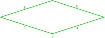
Figure 11: The thin rhombus $\Delta_{r}^{4}$

The corresponding inward–pointing vectors are given by $X_{1}=Y_{1}$, $X_{2}=-Y_{1}$, $X_{3}=Y_{4}$, $X_{4}=-Y_{4}$, while $\lambda_{1}=\lambda_{4}=0$, and $\lambda_{2}=\lambda_{3}=-\frac{1}{2\phi}\sqrt{2+\phi}$. Let us consider the linear mapping defined by

$$\begin{array}[]{cccc}\sigma\colon&\mbox{\bbb{R}}^{4}&\rightarrow&\mbox{\bbb{R}}^{2}\\ &e_{i}&\mapsto&X_{i}.\end{array}$$

Its kernel, l, is the $2$–dimensional subspace of $\mbox{\bbb{R}}^{4}$ that is spanned by $e_{1}+e_{2}$ and $e_{3}+e_{4}$. It is the Lie algebra of $L=\{\,\exp(X)\in T^{4}\,|\,X\in\mbox{\bbb{R}}^{4},\sigma(X)\in Q\,\}$. If $\Psi$ is the moment mapping of the induced $L$ action, then

$$\Psi(z_{1},z_{2},z_{3},z_{4})=\left(|z_{1}|^{2}+|z_{2}|^{2}-\frac{1}{2\phi}\sqrt{2+\phi},|z_{3}|^{2}+|z_{4}|^{2}-\frac{1}{2\phi}\sqrt{2+\phi}\right).$$

Let $r=\left(\frac{1}{2\phi}\sqrt{2+\phi}\right)^{1/2}$ and denote by $S^{3}_{r}$ and $S^{2}_{r}$ the spheres of radius $r$, centered at the origin, of dimension $3$ and $2$ respectively. Then $\Psi^{-1}(0)=S_{r}^{3}\times S_{r}^{3}$. A straightforward computation, using the relations (5), with $k=4$, gives that

$$L=\left\{\,\exp(X)\in T^{4}\,|\,X=\left(s,s+h\phi,t,t+k\phi\right),s,t\in\mbox{\bbb{R}},h,k\in\mbox{\bbb{Z}}\,\right\}=N.$$

In conclusion

$$M_{r}=\frac{\Psi^{-1}(0)}{N}=\frac{S_{r}^{3}\times S_{r}^{3}}{N}=\frac{S_{r}^{2}\times S_{r}^{2}}{\Gamma}$$

and the quasitorus

$$D^{2}=\mbox{\bbb{R}}^{2}/Q$$

acts on $M_{r}$ in a Hamiltonian fashion, with image of the corresponding moment mapping yielding exactly $\Delta_{r}^{2}$. Notice that the quasitorus $D^{2}$ is the same for both the thick and thin rhombuses.

4 Symplectic Interpretation of the Tiling

Recall that we denoted by $M_{R}$ the symplectic quasifold associated to the thick rhombus $\Delta_{R}^{2}$ and by $M_{r}$ the symplectic quasifold associated with the thin rhombus $\Delta_{r}^{4}$. Consider the five distinguished thick rhombuses $\Delta_{R}^{k}$ and the five distinguished thin rhombuses $\Delta_{r}^{k}$, $k=0,\dots,4$. Recall that each of these rhombuses has a natural choice of inward–pointing vectors, these are $\pm Y_{k},\pm Y_{k+1}$ for $\Delta^{k}_{R}$, and $\pm Y_{k},\pm Y_{k+2}$ for $\Delta_{r}^{k}$. Consider now a Penrose tiling with edges of length $1$. Remark that, by Proposition 1.3, in our choice of coordinates, each of its rhombuses can be obtained by translation from one of the $10$ rhombuses $\Delta_{R}^{k}$ and $\Delta_{r}^{k}$. We can then prove the following

Theorem 4.1

The compact symplectic quasifold corresponding to each thick rhombus of a Penrose tiling with edges of length $1$ is given by $M_{R}$. The compact symplectic quasifold corresponding to each thin rhombus is given by $M_{r}$.

Proof.  Observe that, for each $k=0,1,3,4$, there exists a rotation $P$ of $\mbox{\bbb{R}}^{2}$ that leaves the quasilattice $Q$ invariant, that sends the orthogonal vectors relative to the rhombus $\Delta_{R}^{k}$ to the orthogonal vectors relative to the rhombus $\Delta_{R}^{2}$, and such that the dual transformation $P^{*}$ sends the rhombus $\Delta_{R}^{2}$ to the rhombus $\Delta_{R}^{k}$. This implies that the reduced space corresponding to each of the $5$ rhombuses $\Delta_{R}^{k}$, $k=0,\ldots,4$, with the choice of orthogonal vectors and quasilattice specified above, is exactly $M_{R}$. This yields a unique symplectic quasifold, $M_{R}$, for all the rhombuses considered. We argue in the same way for each thin rhombus $\Delta_{r}^{k}$, $k=0,\ldots,4$. Finally, translating the rhombuses $\Delta_{R}^{k}$ does not produce any change in the corresponding quotient spaces, therefore, by Proposition 1.3 we are done.  $\sqcap$$\sqcup$

Theorem 4.2

The quasifolds $M_{R}$ and $M_{r}$ are diffeomorphic but not symplectomorphic.

Proof.  We recall from [14] that a quasifold diffeomorphism, $f$, is a bijective mapping such that, for each point $p\in M_{R}$, there is a local model $W$ around $p$ and a local model $f(W)$ around $f(p)$ such that the mapping $f$, restricted to $W$, is a diffeomorphism of models as given by Definition 2.4. A local model is a submodel of a chart of the atlas that defines the quasifold structure. It is straightforward to check that, since the manifolds $S^{2}_{R}\times S^{2}_{R}$ and $S^{2}_{r}\times S^{2}_{r}$ are diffeomorphic, the quasifolds $M_{R}=(S^{2}_{R}\times S^{2}_{R})/\Gamma$ and $M_{r}=(S^{2}_{r}\times S^{2}_{r})/\Gamma$ are diffeomorphic.

We prove now that $M_{R}$ and $M_{r}$ are not symplectomorphic. Denote by $\omega_{R}$ and $\omega_{r}$ the symplectic forms of $M_{R}$ and $M_{r}$ respectively. Suppose that there is a symplectomorphism $h:M_{R}\longrightarrow M_{r}$, namely a diffeomorphism $h$ such that $h^{*}(\omega_{r})=\omega_{R}$. The quasifold structures on $M_{R}$ and $M_{r}$ are each defined by four charts, one corresponding to each vertex of the rhombus, as shown in Subsection 3.1. We recall from Remark 2.9 that to each point $p\in M_{R}$ one can associate finitely generated groups $\Gamma_{p}$ and $\Lambda_{h(p)}$. It is easy to check, using Lemma 2.6, that the fact that $h$ is a diffeomorphism implies that these two groups are isomorphic. It follows from this that $h$ defines a one–to–one correspondence between the above–given charts of $M_{R}$ and $M_{r}$, and that it sends each of the charts of $M_{R}$ diffeomorphically onto the corresponding chart of $M_{r}$.

Consider now the restriction of $h$ to one such chart of $M_{R}$, say $U_{1,4}$, we want to prove that we can construct a diffeomorphism $\bar{h}$ from $B_{R}\times B_{R}$ to $B_{r}\times B_{r}$ that lifts the restriction of $h$ to the given chart. Notice that all submodels of $U_{1,4}$ are of the type $\tilde{W}/\Gamma_{1,4}$, where $\tilde{W}$ is an open subset of $B_{R}\times B_{R}$ which, since it is $\Gamma_{1,4}$–invariant, can either be the product of two open disks, or the product of an open disk by an open annulus or the product of two open annuli. Therefore a local model around the point $[\tau_{1,4}(0,0)]$ is given by $\tilde{W}_{0}=B_{\delta}\times B_{\delta}$, for a suitable $\delta<R$, modulo the action of $\Gamma_{1,4}$. Since $\tilde{W}_{0}$ is simply connected here a lift of $h$ is well defined. Moreover, it follows from the fact that $\phi$ is irrational that when a lift is well defined on one point of a local model $\tilde{W}$ where the action of $\Gamma_{1,4}$ is free, then it is well defined on all of $\tilde{W}$, without the need of taking a covering of $\tilde{W}/\Gamma_{1,4}$. Finally, observe that if two submodels $\tilde{W}_{1}$ and $\tilde{W}_{2}$ overlap and there is a lift of $h$ defined on each of them, then by Lemma 2.5, there is a unique lift defined on $\tilde{W}_{1}\cup\tilde{W}_{2}$. Now the lift $\bar{h}$ from $B_{R}\times B_{R}$ to $B_{r}\times B_{r}$ can be constructed by gluing the local lifts of $h$ that are defined on suitable submodels of $U_{1,4}$.

Observe now that the four charts of $M_{R}$ intersect in the $4$–dimensional dense open subset where the action of the quasitorus $D^{2}$ is free; then Lemma 2.5 together with diagram (8) allow us to lift the diffeomorphism $h$ to a global diffeomorphism $\tilde{h}$ from $S^{2}_{R}\times S^{2}_{R}$ to $S^{2}_{r}\times S^{2}_{r}$ that is equivariant with respect to the actions of $\Gamma$ and $\Lambda$ respectively. Moreover, since diagram (8) preserves the symplectic structures, we have that $\tilde{h}$ is a symplectomorphism between $S^{2}_{R}\times S^{2}_{R}$ to $S^{2}_{r}\times S^{2}_{r}$, which is impossible.  $\sqcap$$\sqcup$

In conclusion there is a unique quasifold structure that is naturally associated to the Penrose rhombus tiling, and two distinct symplectic structures that distinguish the thick and the thin rhombuses.

Dipartimento di Matematica Applicata ”G. Sansone”, Università di Firenze, Via S. Marta 3, 50139 Firenze, Italy,
E-mail address: fiammetta.battaglia@unifi.it

Dipartimento di Matematica e Applicazioni per l’Architettura, Università di Firenze, Piazza Ghiberti 27, 50122 Firenze, Italy,
E-mail address: elisa.prato@unifi.it

References

- [1] M. Atiyah, Convexity and commuting Hamiltonians, Bull. London Math. Soc. 14 (1982), 1–15.
- [2] D. Austin, Penrose Tiles Talk Across Miles, http://www.ams.org/featurecolumn/archive/penrose.html, last accessed November 11, 2007.
- [3] D. Austin, Penrose Tilings Tied up in Ribbons, http://www.ams.org/featurecolumn/archive/ribbons.html, last accessed November 11, 2007.
- [4] F. Battaglia, E. Prato, The Symplectic Penrose Kite, preprint arXiv:0712.1978v1 [math.SG] (2007).
- [5] F. Battaglia, E. Prato, Quasicrystals and Symplectic Geometry, in preparation.
- [6] T. Delzant, Hamiltoniennes Périodiques et Image Convexe de l’Application Moment, Bull. S.M.F. 116 (1988), 315–339.
- [7] B. Grünbaum, G. C. Shephard, Tilings and patterns, Freeman, New York, 1987.
- [8] V. Guillemin and S. Sternberg, Convexity properties of the moment mapping, Invent. Math. 67 (1982), 491–513.
- [9] E. Lerman, S. Tolman, Hamiltonian Torus Actions on Symplectic Orbifolds and Toric Varieties, Trans. Amer. Math. Soc. 349 (1997), 4201–4230.
- [10] M. Livio, The Golden Ratio: The Story of Phi, the World’s Most Astonishing Number, Broadway Books (2003).
- [11] R. Penrose, The Rôle of Æsthetics in Pure and Applied Mathematical Research, Bull. Inst. Math. Applications, 10 (1974), 266–271.
- [12] R. Penrose, Tilings and Quasicrystals: a Nonlocal Growth Problem?, in Introduction to the Mathematics of Quasicrystals, edited by Marko Jaric, Academic Press, 1989, 53–80.
- [13] R. Penrose, The Emperor’s New Mind, Oxford University Press (2002).
- [14] E. Prato, Simple Non–Rational Convex Polytopes via Symplectic Geometry, Topology 40 (2001), 961–975.
- [15] E. Prato, The Pentagram: From the Goddess to Symplectic Geometry, Proc. Bridges 2007, 123–126.
- [16] M. Senechal, Quasicrystals and Geometry, Cambridge University Press, Cambridge, 1995.
- [17] D. Shechtman, I. Blech, D. Gratias, J. W. Cahn, Metallic Phase with Long–Range Orientational Order and no Translational Symmetry. Phys. Rev. Lett. 53 (1984), 1951–1953.