Eclipsing binary stars in the Large and Small Magellanic Clouds from the MACHO project: The Sample

Abstract

We present a new sample of $4634$ eclipsing binary stars in the Large Magellanic Cloud (LMC), expanding on a previous sample of 611 objects and a new sample of $1509$ eclipsing binary stars in the Small Magellanic Cloud (SMC), that were identified in the light curve database of the MACHO project. We perform a cross correlation with the OGLE-II LMC sample, finding 1236 matches. A cross correlation with the OGLE-II SMC sample finds 698 matches. We then compare the LMC subsamples corresponding to center and the periphery of the LMC and find only minor differences between the two populations. These samples are sufficiently large and complete that statistical studies of the binary star populations are possible.

1 Introduction

Eclipsing binary stars (EBs) are important for astrophysical research in many ways. They may be used to obtain accurate estimates of star masses and radii (Andersen, 1991, and references therein). Precise determination of stellar parameters can in turn be used to put theories of stellar structure and evolution to a stringent test by comparing measured parameters with theoretical predictions (Lastennet & Valls-Gabaud, 2002; Lastennet et al., 2003, and references therein).

EBs may also be used for distance determination and this use goes back several decades; its history is reviewed by Kruszewski & Semeniuk (1999). Since Stebbins (1911) used an estimate of the parallax to $\beta$ Aurigæ to infer the surface brightness of both its components, it has been known that a good photometric light curve plus a double line spectroscopic orbit admits a simple geometric relationship between the surface brightnesses of the stars and the distance to the EB; Stebbins (1911) however had no way at the time to make the reverse “surface brightness to distance” inference and his paper does no mention this possibility. After Stebbins (1911), other early papers (Gaposchkin, 1933; Woolley, 1934; Pilowski, 1936; Kopal, 1939; Gaposchkin, 1938, 1940) used parallaxes obtained independently to estimate surface brightnesses, but, as remarked by Kruszewski & Semeniuk (1999), these pioneers surely knew of the potential of this technique to estimate distances. Modern analyses of EBs have usually focussed on this technique (e.g. Andersen (1991)). The method affords high precision due to its purely geometrical nature and has been applied by a number of authors to determine the distance to the Large Magellanic Cloud (LMC) using HV2274 (Udalski et al., 1998a; Guinan et al., 1998; Nelson et al., 2000; Groenewegen & Salaris, 2001), HV982 (Fizpatrick et al., 2002), EROS 1044 (Ribas et al., 2002) and HV 5936 (Fitzpatrick et. al., 2003); an attempt to use EBs to determine the distance to M31 is currently under way (Ribas et al., 2003) and the DIRECT project is attempting to measure the distance to M31 and M33 via EBs and Cepheids (Kaluzny et al., 1998; Bonanos et al., 2003; Bonanos, 2005); other recent examples include Michalska & Pigulski (2005) who present a sample of detached binaries in the LMC for distance determination and Ribas et al. (2005) who present the first determination of the distance and properties of an EB in M31; North (2006) presents a sample of EBs with total eclipses in the LMC suitable for spectroscopic studies. In general it is important that distances be determined using a large sample of EBs to minimize the impact of systematic errors. A recent collection of references on extragalactic binaries can be found in Ribas & Gimenez (2004).

Large-scale surveys to detect gravitational microlensing events have identified and collected light curves for large numbers of variable stars in the bulge of the Milky Way and in the Magellanic Clouds. Eclipsing binary stars comprise a significant fraction of these collections. The MACHO collaboration has presented a sample of 611 EBs in the LMC with preliminary analyses of their orbits (Alcock et al., 1997a). A catalogue of $3031$ EBs in the LMC found in the MACHO database has been just published by Derekas, Kiss, & Bedding (2007); this catalogue was compiled by analyzing a list of $6835$ stars classified as possible EBs in the MACHO database; a cross correlation between these $6835$ stars and our sample finds just $1987$ matches, thus at least about $2700$ EBs in our catalogue are new identifications. The $6835$ classified as possible EBs were found in regions of parameter space such as color, magnitude, and period, where one does not expect to find pulsating variables and therefore the detected variability of these stars was tentatively ascribed to eclipses. Regions where pulsating variables could exist were not considered while making this preliminary classification and EBs there were therefore not included in the list. In our search we did not rely primarily on cuts in parameter space and and we did not exclude a priori regions of this space where pulsating variables are present; therefore we were able to classify many EBs in these regions, that were not included in the preliminary classification. The OGLE collaboration has introduced a sample of $2580$ EBs in the LMC (Wyrzykowski et al., 2003) and of $1351$ EBs in the Small Magellanic Cloud (SMC: Wyrzykowski et al., 2004). Both samples were selected from their catalogue of variable stars in the Magellanic Clouds (Żebruń et al., 2001) compiled from observations taken during the second part of the project (OGLE II: Udalski, Kubiak & Szymański, 1997) and reduced via Difference Image Analysis (DIA: Żebruń, Soszyński, & Woz̀niak, 2001). An earlier sample of $79$ EBs in the bar of the LMC was presented by the EROS collaboration(Grison et al., 1995). Other large variable star data sets are being produced by surveys not specifically designed to detect gravitational microlensing, such as the All Sky Automated Survey (ASAS: Pojmański, 1997) .

The availability of large samples of EBs (and the even larger ones that can be found by future surveys such as Pan-STARRS and LSST) can have an important impact on stellar astrophysics. This impact can arise in two qualitatively different approaches. First, a large catalogue allows the discerning researcher to select carefully a few EBs for detailed follow-up study; the distance estimation described above is an example of this. Second, statistical analyses of an entire population become possible when a large collection is assembled; such analyses of EBs have not previously been possible. To fulfill this promise there are challenges to overcome, including finding EBs in large data sets and automating their analysis. With regard to the first task, the discovery problem is complicated by the fact that EBs do not have clear relationships between their parameters (period, luminosity, colors) as do the major classes of pulsating variables. This makes it difficult to find them via simple and well understood cuts in parameter space. The first step toward automated discovery is thus to have a large sample of data on which to experiment with search techniques. This non-trivial exercise in mining large data sets can be useful for future surveys that are not necessarily aimed at binary star research. An example is given by Wyrzykowski et al. (2003) and Wyrzykowski et al. (2004) who employ an artificial neural network to identify EBs in the OGLE-II LMC and SMC samples, but more needs to be done. With regard to analysis of EBs, the traditional approach has been to carefully analyze individual systems with the help of dedicated computer codes such as the Wilson-Devinney code (WD: Wilson & Devinney, 1971; Wilson, 1979). This becomes impracticable when many thousands of stars are involved and an automated approach is required. The light curves in a previous sample of 1459 EBs in the SMC found by OGLE-II (Udalski et al., 1998b) were systematically solved by Wyithe & Wilson (2001, 2002) using an automated version of the WD code; the ASAS collaboration has developed an automated classification algorithm for variable stars based on Fourier decomposition (Pojmański, 2002); Devor (2005) found and analyzed 10000 Bulge EBs from OGLE-II using DEBiL, an EB analysis code that allows automated solutions of large EB data sets and works best for detached EBs; a genetic algorithm based approach to finding good initial parameters for WD is described in Metcalfe (1999).

This paper is the first of a series of papers aimed at describing the EB samples in the MACHO database and is organized as follows: Section 2 introduces the LMC and SMC samples; Section 3 describes the Color Magnitude Diagram (CMD) and the Color Period Diagram, pointing out significant features in them, Section 4 compares the LMC and SMC samples, Section 5 describes the results of the cross correlation with the OGLE LMC and SMC samples, and Section 6 reports where and in what form the data presented in the paper can be accessed on line.

2 The Samples

2.1 The MACHO Project

The MACHO Project was an astronomical survey whose primary aim was to detect gravitational microlensing events of background sources by compact objects in the halo of the Milky Way. The gravitational background sources were located in the LMC, SMC and the bulge of the Milky Way; more details on the detection of microlensing events can be found in Alcock et al. (2000a) and references therein. Observations were carried out from July 1992 to December 1999 with the dedicated $1.27\mathrm{m}$ telescope of Mount Stromlo, Australia, using a $2\times 2$ mosaic of $2048\times 2048$ CCD in two bandpasses simultaneously. These are called MACHO “blue”, hereafter indicated with $V_{\mathrm{MACHO}}$, with a bandpass of $\sim 440-590\mathrm{nm}$ and MACHO “red”, hereafter indicated with $R_{\mathrm{MACHO}}$, with a bandpass of $\sim 590-780\mathrm{nm}$; these widths are between the half-response points as estimated from Figure $1$ of (Alcock et al., 1999). The bandpasses and the transformations to standard Johnson $V$ and Cousins $R$ bands are described in detail in (Alcock et al., 1999); see in particular their Figure $1$ for the instrumental throughput of the two MACHO bands. Each MACHO object is identified by its field number ($1-82$ for the LMC, $201-213$ for the SMC), its tile number (which can overlap more than one field), and its sequence number in the tile. These form the so called MACHO Field.Tile.Sequence (FTS), which is used in this paper to label EBs. Note that, since some overlap exists between fields, one star may have two or more FTS identifiers.

2.2 The Large Magellanic Cloud Sample

The LMC sample we present comprises $4634$ EBs selected by a variety of methods which we describe in this section; the sample includes the 611 EBs described in Alcock et al. (1997a). The LMC magnitudes quoted in this paper have been obtained by using the following transformation:

$$V = V_{\mathrm{MACHO}}+24.22~{}\mathrm{mag}-0.18(V_{\mathrm{MACHO}}-R_{\mathrm{MACHO}})$$

$$R = R_{\mathrm{MACHO}}+23.98~{}\mathrm{mag}+0.18(V_{\mathrm{MACHO}}-R_{\mathrm{MACHO}}).$$ (1)

From now on we will use the symbols $V$, $R$, and $\vr$ to refer to standard magnitudes obtained from $V_{\mathrm{MACHO}}$ and $R_{\mathrm{MACHO}}$ via Eq. 2.2 for the LMC and Eq. 2.7 for the SMC, and not corrected for reddening; we will also use $V_{\mathrm{MACHO}}$ and $R_{\mathrm{MACHO}}$ to indicate instrumental magnitudes. The observations number in several hundreds in both bandpasses for most light curves; Figure 1 shows histograms of the number of light curve points of the EBs in both bands; the $V_{\mathrm{MACHO}}$ band has on average more observations than the $R_{\mathrm{MACHO}}$ band because one half of one of the red CCDs was out of commission during part of the project. The central fields of the LMC were observed more often and the periphery less often as shown by the three peaks in the distribution where the first peak corresponds to the LMC periphery and the other two correspond to the center.

Figure 1: Histograms of the number of light curve points for both bands for the LMC sample. The first peak corresponds to objects in the LMC periphery which was observed less often than the center, the other two peaks to the regions in and near the central bar.

2.3 Identifying Eclipsing Binary Stars in the MACHO database

This Section describes the techniques employed to identify EBs both in the LMC and in the SMC; the results we quote are relative to the LMC. From now on we will always use the term unfolded light curve to indicate a set of time ordered observations and will reserve the term light curve to indicate a set of time ordered observations folded (or phased) around a period, omitting for brevity the adjectives “folded” and “phased”; we will also use the terms EB, system, and object interchangeably.

All sources in the survey were subjected to a test for variability (Cook et al., 1995) and a large number of variable sources were identified (Alcock at al., 1995; Alcock et al., 1996a, b, 1997b). This first test starts by first eliminating the $20\%$ most extreme photometric data points; the resulting unfolded light curve is fitted to constant brightness and its $\chi^{2}$/dof is calculated. The elimination of the most extreme points is expected to reduce the influence of noise and yield a good fit for a constant source, but not for a truly variable one. We consider the source variable if the $\chi^{2}$/dof thus computed can occur by chance with probability $1\%$ or less. Sources that were flagged for variability were tested for periodicity. Periods were found using the Supersmoother algorithm (Reimann, 1994, first published by Friedman (1984)). The algorithm folds the unfolded light curve around trial periods and selects those periods in which the smoothed light curve matches the data best in a statistical sense; we have selected the best 15 possible periods ranked by the smoothness of the light curve. Periods were found separately for the red and blue unfolded light curves. The period selected as the best one by the program turned out to be “correct” in $88\%$ of the EBs for at least one band; for $10\%$ of the EBs the second best period turned out to be correct for at least one band and only for $<0.5\%$ of the EBs did the procedure fail to find a good period. In these cases “correctness” was determined by direct visual inspection.

Table 1: Period determination via Supersmoother.

Color	Number of EBs	$P$$=P_{\mathrm{SS}}$	$P$$=2P_{\mathrm{SS}}$	$P$$=P_{\mathrm{SS}}/2$	Other
Red	$4634$	$3432$	$604$	$103$	$495$
		$74\%$	$13\%$	$2\%$	$11\%$
Blue	$4634$	$3460$	$583$	$108$	$483$
		$75\%$	$13\%$	$2\%$	$10\%$

The Supersmoother program can fail in two manners when fitting EBs. First when one eclipse (the secondary) is very shallow, Supersmoother may not recognize it and yield a period twice the correct one. Second, when the two eclipses have nearly equal depth Supersmoother may confuse the secondary and the primary eclipses yielding a period half the correct one. The first failure happened, for one or both bands, in about $2\%$ of EBs, whereas the second happened in about $13\%$ of EBs. These cases are easy to correct upon visual inspection. For $\sim 100$ EBs Supersmoother gave a period which was some other multiple of the correct one for at least one band; these were fixed upon visual inspection. For the remaining EBs we tried folding the light curves around the other periods selected by Supersmoother and managed to identify the correct period for most of them. In $27$ cases in which there were OGLE-II counterparts we adopted OGLE periods since, though differing in some cases by less than $1\%$ from the periods found by Supersmoother, they gave a much better light curve. We found $51$ stars in which the secondary eclipse was not evident, either because it was shallow or because the light curve was noisy, but with an OGLE-II counterpart in which it was clearly visible; these stars have not been included in the catalogue. The periods in the two bands differ on average by $0.02\%$. These results are summarized in Table 1.

The search for variable objects in the LMC gave $\sim 207,000$ objects of which $\sim 66,000$ were found to be periodic. To find EBs in this sample we considered a variety of properties of light curves. The techniques we employed are:

1. Look at the number of photometric excursions (“dips”) in the light curve. An EB is expected to show two “dips” in an entire period corresponding to the two eclipses as opposed to a Cepheid or an RRLyræ star for which only one is expected. The number of photometric excursions was calculated by Supersmoother by counting the number of times the smoothed light curve crosses the mean: we selected stars with two excursions in both bands. We additionally imposed a cut on light curve amplitudes: calling $\mathrm{Ampl_{V}}$ and $\mathrm{Ampl_{R}}$ the amplitudes of the blue and red light curves respectively, as computed by Supersmoother, we imposed $\mathrm{Ampl_{V}}/\mathrm{Ampl_{R}}<1.2$. This amplitude cut was imposed to help in eliminating RRLyræs from the sample, since, considering a population of several thousands probable RRLyræs found in the MACHO database, we found that, on average, $\mathrm{Ampl_{V}}/\mathrm{Ampl_{R}}\sim 1.27$; imposing a cut $\mathrm{Ampl_{V}}/\mathrm{Ampl_{R}}<1.2$ should therefore filter out many RRLyræ. In our sample just $2421$ EBs ($\sim 52\%$) pass this cut; we then removed the amplitude cut and look at the number of photometric excursions alone we found that $3039$ EBs ($\sim 66\%$) pass this relaxed cut.

2. Look at the ratio of number of points five standard deviations away ($\mathrm{s}5$) from the median to the number of points five standard deviations below the median ($\mathrm{s}5\mathrm{d}$). This ratio is expected to be $\sim 2$ for a typical single variable star. For an EB we expect this ratio to approach $\sim 1$ as the signal to noise in the photometry increases, as most “outlier” points are due to eclipses. We imposed a cut $\mathrm{s}5/\mathrm{s}5\mathrm{d}<1.2$ in both bands and found that $3417$ EBs pass it ($\sim 74\%$), whereas for the overall variable star dataset the figure is $\sim 19,600$ out of $66,000$ or $\sim 30\%$.

3. Use a decision tree. We applied the decision tree program described in Murthy, Kasif & Salzberg (1994), which was run on all the variable objects on the catalogue and gave for each the probability that it was an EB, an RRLyræ, a Cepheid, a long period variable or an unknown object. In all $\sim 17000$ objects were found most likely by the decision tree to be EBs but only $3281$ were found to be real on visual inspection and included in the sample.

4. Use a similarity technique. We finally tested the sample with a technique described in Protopapas et al. (2006) aimed at finding “outliers” in large data sets of variable star light curves. The technique aims at finding objects whose light curves are most dissimilar, in a statistical sense, from an “average” light curve built out of all the light curve in the data set. This is accomplished by looking at all the pairs of light curves to find their mutual similarity as defined in Protopapas et al. (2006) and, for each light curve, by then combining these measures, to find its overall similarity to the rest of the sample. Light curves with low measure of similarity are flagged as outliers. This approach was useful in finding misfolded lightcurves since it found many objects for which the period for one band gave a badly folded light curve but the period for the other band gave a good folding. This happened for $198$ EBs, despite these periods differing on average by just $0.18\%$; in this case we selected the period that gave the good light curve for both bands.

Since all the techniques we used give some false positives, each candidate was also visually inspected before inclusion in the sample; we paid closer attention to those stars which could more easily be classified as EBs without being so, like ellipsoidal variables (see Subsection 2.6) and Cepheids and RRLyræ mistakenly folded around a period twice their real one.

Table 2: Summary of cuts applied to define the LMC sample.

	Number of EBs	$2$ dips	$2$ dips and $\mathrm{Ampl_{V}}<1.2\mathrm{Ampl_{R}}$	$\mathrm{s}5/\mathrm{s}5\mathrm{d}<1.2$	Decision tree
EB	$4634$	$3039$	$2421$	$3417$	$3281$
		$66\%$	$52\%$	$74\%$	$71\%$
All variable sources	$\sim 66,000$	$\sim 8000$	$\sim 7300$	$\sim 19,600$	$\sim 7900$
		$\sim 12\%$	$\sim 11\%$	$\sim 30\%$	$\sim 12\%$

Table 3: Summary of EBs passing more than one cut.

Cuts	Number of EBs
$2$ dips and $\mathrm{s}5/\mathrm{s}5\mathrm{d}<1.2$	$2061$
$2$ dips, $\mathrm{Ampl_{V}}<1.2\mathrm{Ampl_{R}}$, and $\mathrm{s}5/\mathrm{s}5\mathrm{d}<1.2$	$1686$
$2$ dips and decision tree	$2031$
$\mathrm{s}5/\mathrm{s}5\mathrm{d}<1.2$, and decision tree	$2574$
$2$ dips, $\mathrm{Ampl_{V}}<1.2\mathrm{Ampl_{R}}$, and decision tree	$1761$
$2$ dips, $\mathrm{s}5/\mathrm{s}5\mathrm{d}<1.2$, and decision tree	$1488$
$2$ dips, $\mathrm{Ampl_{V}}<1.2\mathrm{Ampl_{R}}$, $\mathrm{s}5/\mathrm{s}5\mathrm{d}<1.2$, and decision tree	$1280$

These results of our search techniques are summarized in Table 2, and Table 3 shows the number of EBs that pass more than one cut. As the numbers show these heuristic tests are far from perfect and tend to give too many candidates; however we feel that the large dimension of our sample can allow the determination of more stringent tests, an absolute necessity for the analysis of future surveys.

Our search gave $266$ objects observed in more than one field: these duplicates have different MACHO field numbers, but typically the same tile number. In this case we summed the numbers of observations in both bands for each field and chose the one which had the highest total number of observations: the object is identified by that corresponding FTS only.

Figure 2 shows a logarithmic histogram of the period distribution. Note that the periods range from a fraction of a day to several hundreds of days. Figure 3 shows a histogram of the distribution of median $V$, $R$ and $\vr$. Note that the magnitudes range in values from $\sim 20~{}\mathrm{mag}$ to $\sim 14~{}\mathrm{mag}$ both in $V$ and $R$ with a peak around $18~{}\mathrm{mag}$.

Figure 2: Period histogram for $4634$ EBs in the LMC sample; the distribution peaks strongly in the $0.8-4\mathrm{d}$ range and has a tail in the $10-100\mathrm{d}$ range. The size of the bins is $\sim 1/100$ of the span of the logarithms of the periods.

Figure 3: Standard $V$ and $R$ magnitudes and $\vr$ histograms for the LMC sample; the bin size is $0.1~{}\mathrm{mag}$ for the $V$ and $R$ histograms and $0.01~{}\mathrm{mag}$ for the $\vr$ one. The $\vr$ histogram is strongly peaked around $\vr\sim 0~{}\mathrm{mag}$, showing a majority of unevolved EBs, but the longer tail, with the smaller bump around $\vr\sim 0.5~{}\mathrm{mag}$ shows a sizeable minority of fairly evolved systems as also shown by the higher $V$ histogram values around $16~{}\mathrm{mag}$ with respect to the $R$ histogram.

The average photometric error for the LMC is $\sim 0.05~{}\mathrm{mag}$ in both instrumental bands; the average error for a light curve as a function of median relative magnitude is in standard magnitudes is shown in Figure 4.

Figure 4: Errors as a function of median magnitude for the LMC sample.

2.4 Root Mean Square of residuals for the LMC sample

For the LMC sample we estimated the distribution the Root Mean Square (RMS) of the residuals $O_{i}-C_{i}$ of the observations around a theoretical light curve as a function of median relative magnitude where $O_{i}$ is the value of the observed magnitude orbital phase $\phi_{i}$, and $C_{i}$ is the theoretical value at the same phase. Theoretical values were obtained by fitting the light curves using the JKTEBOP code (Southworth, Maxted & Smalley, 2004a; Southworth et al., 2004b). The JKTEBOP code is based on the EBOP code (Etzel, 1981; Popper & Etzel, 1981), which implements the model by Nelson & Davis (1972) with some modifications; JKTEBOP in turn adds several modifications and extensions to the original EBOP code that make it easier to use, especially when fitting a large number of light curves. Before fitting we eliminated outlying points by taking averages of all points in boxes containing from $\sim 10$ to $\sim 20$ points along a light curve and discarding the points more than $2$ standard deviations away from these averages. We obtained starting values for the model parameters by running the DEBiL code (Devor, 2005) and using the values it computed; the limb darkening values for the $V$ and $R$ bands were taken from (Cox, 2000). We fixed the ratio of the masses, $q$, to $1$, $0.1$ and $10$ and did the fit in each case taking in the end the best result. Finally we selected light curves with $\chi^{2}/\mathrm{dof}<2$ to show in Figure 5. Out of $4636$ EBs in the LMC the program converged in $4090$ cases in the $R$ band and in $4312$ cases in the $V$ band; we found $3067$ fits with $\chi^{2}/\mathrm{dof}<2$ in the $R$ band and $3198$ in the $V$ band. We point out that those fits were made only with the aim of obtaining a good theoretical light curve for as many observed light curves as possible in a fast and automated manner, so that a residuals distribution could be calculated. In particular we did not attempt to accurately determine astrophysical parameters for our EBs. This is also the reason why we discarded points at just $2$ standard deviations away from the moving averages, which could result in eliminating potentially interesting information for some EBs; such objects are obviously deserving of more in depth study which we did not attempt here. While in general our fits were good in the case of largely separated, undistorted systems, they were often bad for close, strongly distorted ones, which is to be expected since JKTEBOP is not meant to be used for such systems; also in several cases our fits were bad because the scatter of the observed values was larger than the observational errors, which suggests that other physical phenomena, such as pulsation of one or both components, are present. The RMS distributions of the residuals vs. median magnitudes $V$ and $R$ are shown in Figure 5.

Figure 5: RMS of residuals as a function of median relative magnitude for the LMC sample.

2.5 Examples of light curves

Figures 6, 7, 8, 9, 10, and 11 show some examples of light curves. The panels on the left show the original light curves, those on the right show the light curves with the outlying points removed, the error bars, the theoretical light curves from the fit and the residuals The EBs shown are meant to be representative of the sample, this is why some examples of bad fits are included. Comparing the panels on the left with the panels on the right for these figures gives an idea of the effect of removing outlying points. In particular the figures suggest that for those objects with good fits the procedure resulted in the elimination of truly outlying points; these EBs are mostly detached with undistorted components. For objects with bad fits, which mostly comprise EBs with close and strongly distorted components, the situation is less clear. For example the system labelled 1.3442.172 shown in Figure 7 exhibits some points in the $R$ band, at secondary eclipse around phase $\sim 0.4$, that run almost parallel to the main light curve but at a higher magnitude. Such points may or may not be physically significant; some of these are removed by our procedure, but the fit is nevertheless bad. The systems labelled 1.3804.164 in Figure 9 and 1.4055.98 in Figure 10 show a large and step-like scatter band, the reason of which is, we think, intrinsic variability of the secondary component, as suggested by the fact that the band becomes much narrower at primary eclipse but not at secondary eclipse; this interpretation is also suggested by the fact that the residuals show an oscillating behavior as a function of phase. In both 1.4055.98 and 36.5943.658 in Figure 11 the scatter band is much larger than the observational error which explains their bad fits. These examples show that the samples contain many EBs which could be deserving of more careful study which we did not attempt here. The properties of these EBs are summarized in Table 4; of the $12$ EBs shown $8$ have two photometric excursions in both bands and $\mathrm{Ampl_{V}}/\mathrm{Ampl_{R}}<1.2$, $7$ are found by the decision tree, $5$ have $\mathrm{s}5/\mathrm{s}5\mathrm{d}<1.2$, and $2$ have a counterpart in the OGLE-II sample: 1.3442.172 (counterpart OGLE050149.20-691945.5 in field LMC$\_$SC15) and 1.4055.98 (counterpart OGLE050542.06-684732.8 in field LMC$\_$SC13).

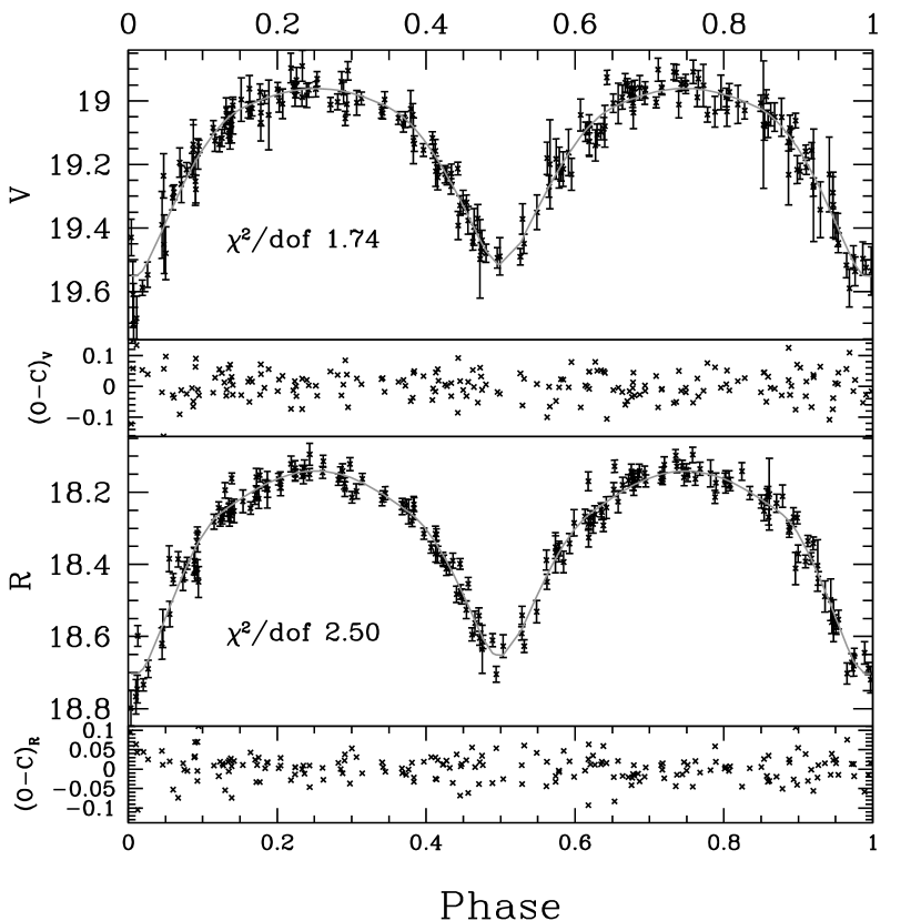
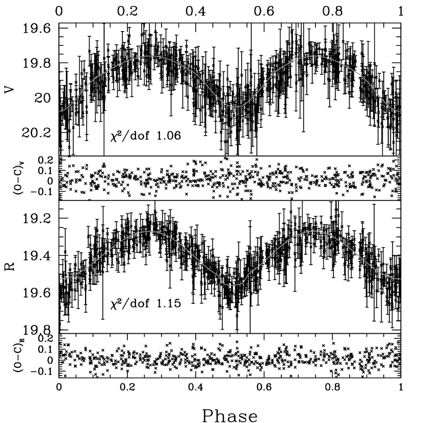
Figure 6: Examples of LMC EBs light curves, arranged by ascending period; for basic data see Table 4. Left: observed light curves with all data points. The arrows show the baseline as defined in Table 4. Right: observed light curves with outlying points removed, theoretical light curves from the fit and residuals.

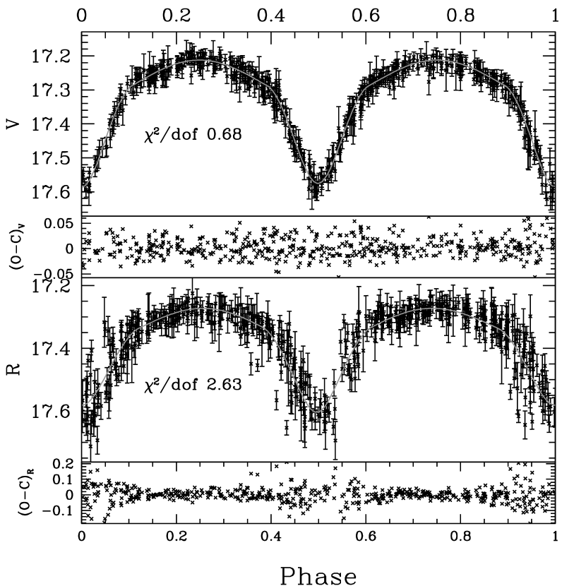
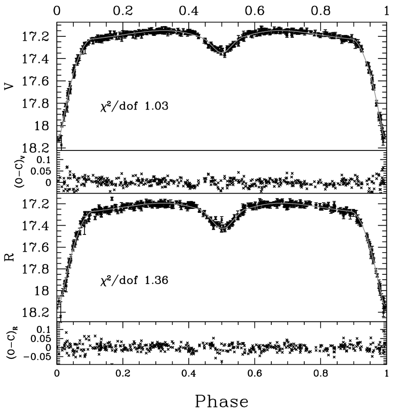
Figure 7: Examples of LMC EBs light curves, arranged by ascending period; for basic data see Table 4. Left: observed light curves with all data points. The arrows show the baseline as defined in Table 4. Right: observed light curves with outlying points removed, theoretical light curves from the fit and residuals.

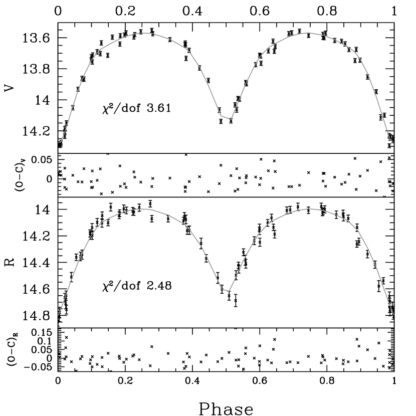
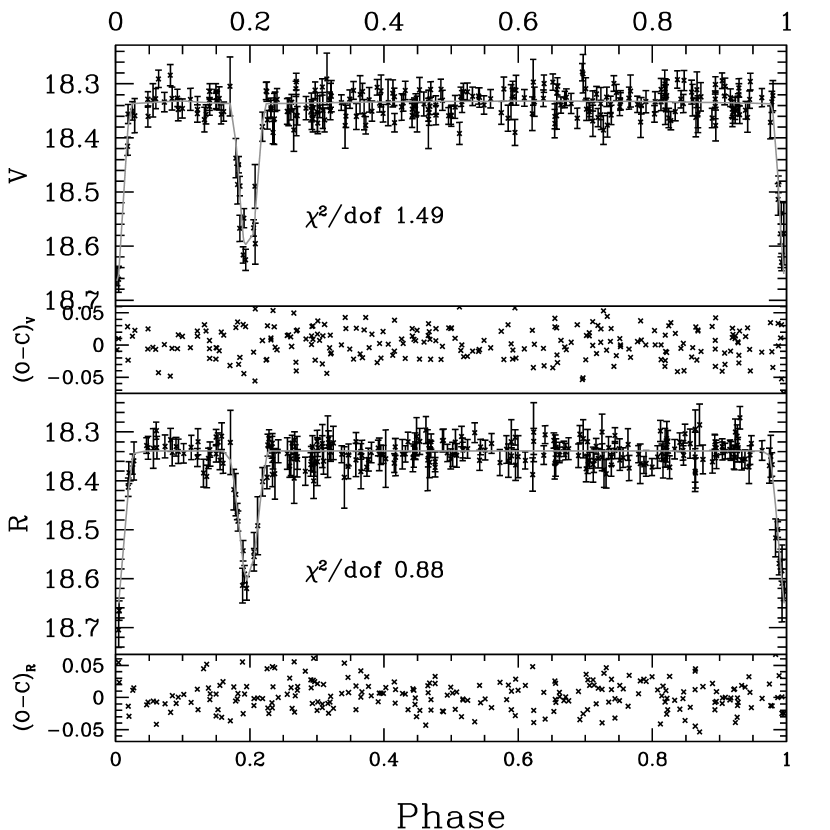
Figure 8: Examples of LMC EBs light curves, arranged by ascending period; for basic data see Table 4. Left: observed light curves with all data points. The arrows show the baseline as defined in Table 4. Right: observed light curves with outlying points removed, theoretical light curves from the fit and residuals.

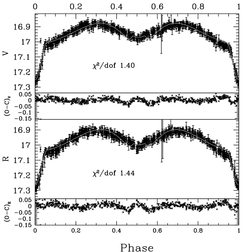
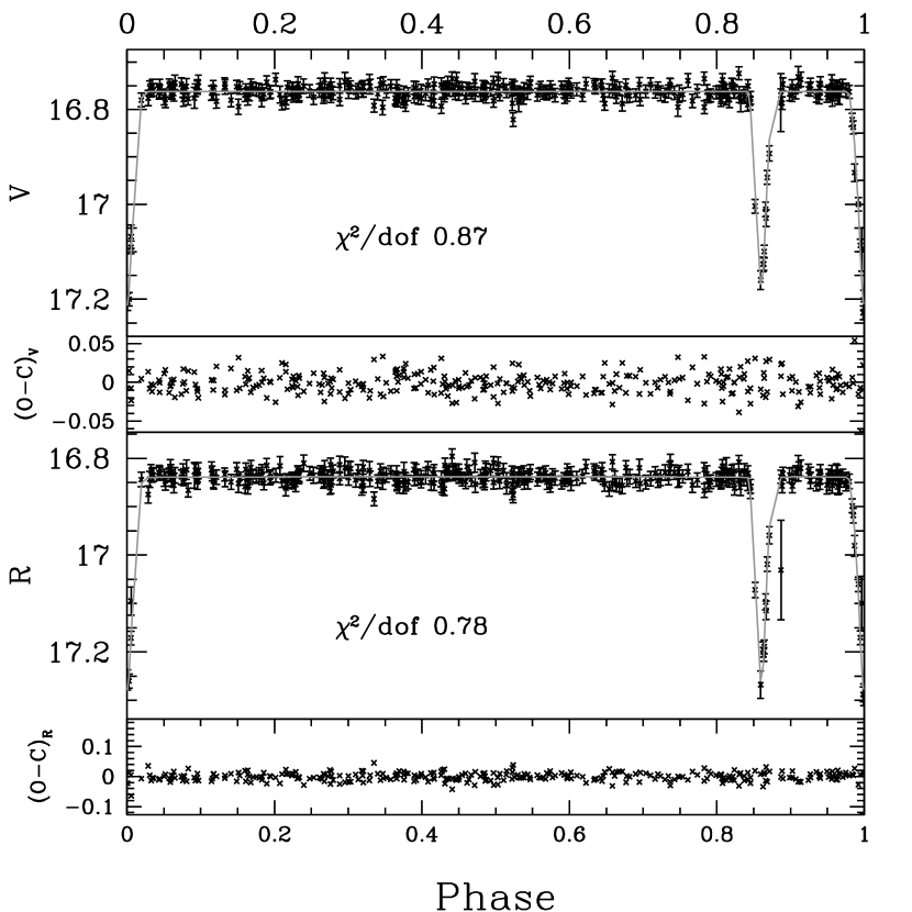
Figure 9: Examples of LMC EBs light curves, arranged by ascending period; for basic data see Table 4. Left: observed light curves with all data points. The arrows show the baseline as defined in Table 4. Right: observed light curves with outlying points removed, theoretical light curves from the fit and residuals.

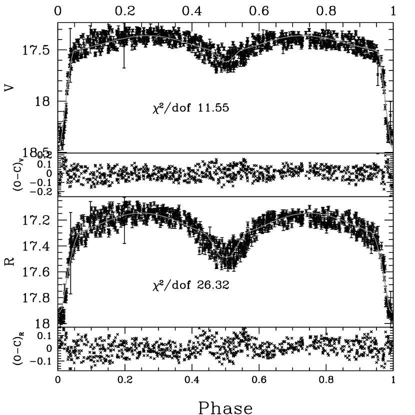
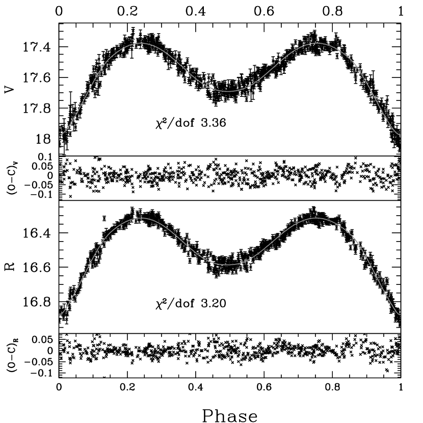
Figure 10: Examples of LMC EBs light curves, arranged by ascending period; for basic data see Table 4. Left: observed light curves with all data points. The arrows show the baseline as defined in Table 4. Right: observed light curves with outlying points removed, theoretical light curves from the fit and residuals.

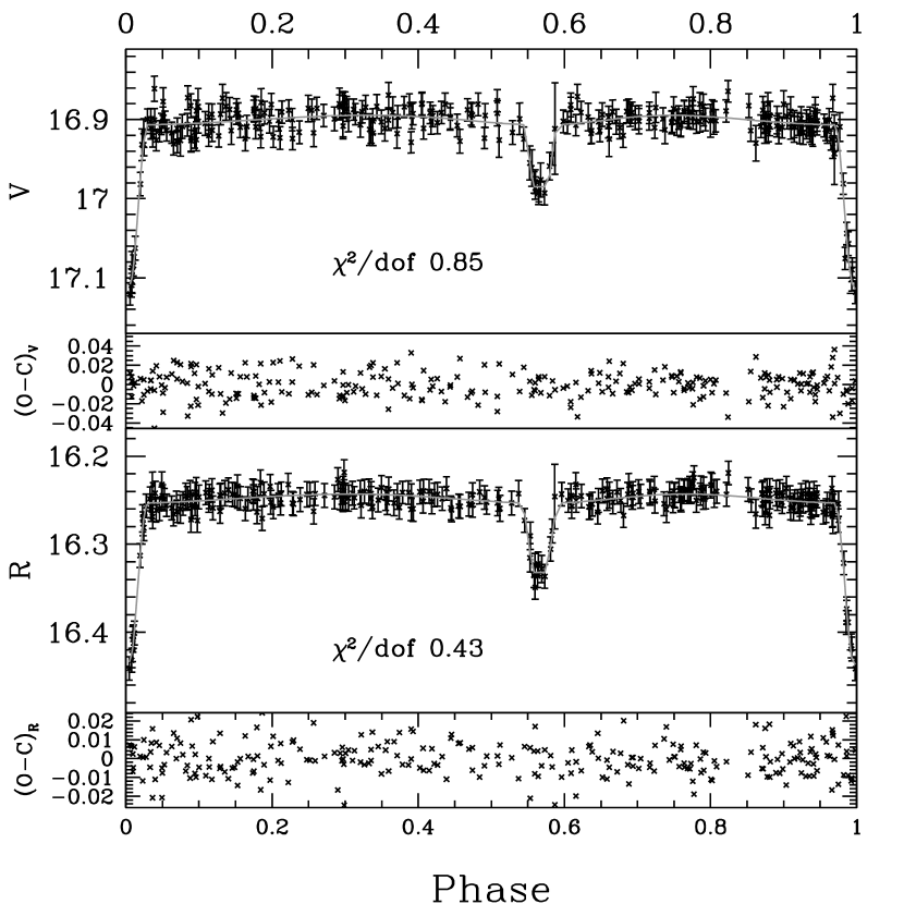
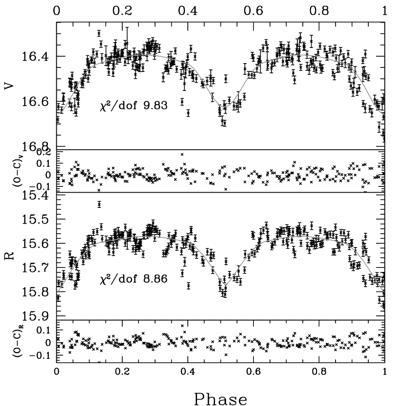
Figure 11: Examples of LMC EBs light curves, arranged by ascending period; for basic data see Table 4. Left: observed light curves with all data points. The arrows show the baseline as defined in Table 4. Right: observed light curves with outlying points removed, theoretical light curves from the fit and residuals.

Table 4: Basic data for the LMC EBs shown in Figs. 6, 7, and 8. The EBs are arranged by ascending period.

MACHO ID	RA(J2000)	DEC(J2000)	Period($\mathrm{d}$)	$V$ baseline	$R$ baseline	$\vr$	Comment
65.8581.67	05:33:09.458	-65:30:29.13	0.19	18.93	18.13	0.8	Shortest period in sample
9.5000.790	05:11:20.548	-70:21:00.16	0.24	19.70	19.23	0.47	Very short period
1.3442.172	05:01:49.005	-69:19:45.60	1.02	17.21	17.26	-0.05	Fairly typical EB
10.4035.145	05:05:02.233	-70:06:13.27	2.53	17.14	17.19	-0.05	Fairly typical EB
68.10843.699	05:47:10.738	-67:58:55.74	3.07	13.56	13.99	-0.43	Bluest in sample
62.7240.102	05:24:55.090	-66:11:55.28	4.17	18.30	18.30	0.00	Very high eccentric orbit
1.3804.164	05:03:36.536	-69:23:32.27	4.19	16.88	16.90	-0.02	Algol type
41.2459.43	04:55:43.321	-70:18:00.44	13.18	16.74	16.82	-0.08	Highest eccentric orbit
1.4055.98	05:05:42.201	-68:47:33.44	24.51	17.32	17.11	0.21	Fairly typical EB
12.10443.34	05:44:47.185	-70:27:26.65	319.37	17.35	16.30	1.05	Reddest in sample
62.6514.2213	05:20:32.499	-66:13:17.92	417.60	16.88	16.23	0.65	Long Period
36.5943.658	05:17:15.478	-71:57:45.69	633.70	16.35	15.54	0.81	Longest Period in sample

The information in Table 4 is also available in its entirety via the link to the machine-readable version above. The EBs are arranged by ascending period. Units of right ascension are hours, minutes, and seconds, and units of declination are degrees, arcminutes, and arcseconds.

2.6 Ellipsoidal variables in the samples

Ellipsoidal variability occurs in a close binary system when one (or both) component(s) is (are) tidally distorted by the companion. If the binary system is detached, as most systems in our samples are, the distorted stars assume the asymmetric, egg like shape of the Roche equipotential surface whereas in the case of contact system the shape of the common equipotential surface is more reminiscent of a dumbbell. The light curve of an ellipsoidal variable system reveals a continuously varying profile, with two maxima and two minima per period, with the minima often having different depth, whereas the maxima are usually equal. The main reason for this variability is that, as the stars rotate, their projected areas on the sky vary, reaching a maximum at the two quadratures and a minimum at the two conjunctions; the measured flux thus varies in the same way during a period. More information on ellipsoidal variables can be found in (Hilditch, 2001) A large sample of ellipsoidal variables in the LMC has been released by the OGLE collaboration (Soszyński et al., 2004); an analysis of ellipsoidal variables found in the MACHO database has been published by Derekas et al. (2006). A binary system can present both eclipses and ellipsoidal variability but in many cases it may not be possible to clearly recognize an eclipse from visual inspection; this poses a problem for the compilation of EB catalogues since the light curves of EBs and non eclipsing ellipsoidal variables can be easily confused.

We looked for possible contamination by ellipsoidal variables in our sample and found $\sim 120$ systems exhibiting ellipsoidal variability which we then visually checked more carefully than other stars which were clearly EBs. We also attempted a less subjective approach by fitting these systems with the EBOP program (Etzel, 1981; Popper & Etzel, 1981; Nelson & Davis, 1972) following the prescriptions of Alcock et al. (1997a); however since EBOP is not designed for analyzing such distorted systems the final decision about whether or not to include a star exhibiting ellipsoidal variability in the sample was taken upon visual inspection. Figure 12 shows two examples of EB systems with pronounced ellipsoidal variability, basic data on these systems are given in Table 5.

Figure 12: Above: light curves for two long period EBs with strong ellipsoidal variability in the LMC sample. Below: light curves of two non eclipsing ellipsoidal variables.

Table 5: Basic data for the LMC ellipsoidal variables shown in Figure 12. The variables are arranged by ascending period.

MACHO ID	RA(J2000)	DEC(J2000)	Period($\mathrm{d}$)	$V$ baseline	$R$ baseline	$\vr$	Eclipsing
1.3934.140	05:04:23.977	-68:49:21.65	85.88	17.68	17.03	0.65	No
58.6147.42	05:18:03.677	-66:27:20.17	105.08	17.78	17.06	0.72	No
15.10916.25	05:47:21.831	-71:10:46.49	355.28	17.04	16.05	0.99	Yes
14.9588.6	05:39:28.498	-71:00:46.01	411.04	14.75	13.95	0.80	Yes

2.7 The Small Magellanic Cloud sample

The SMC sample comprises $1509$ EBs selected via the same techniques as the LMC EBs and confirmed by visual inspection; the general considerations of the preceding subsection regarding search for variability apply here as well. The sky coverage in the SMC corresponds to MACHO fields 206, 207, 208, 211, 212 and 213; field center coordinates for these fields are given in Table 6.

Table 6: MACHO field coordinates for the SMC.

Field ID	RA(J2000)	DEC(J2000)	Date
206	1:05:21.70	-72:26:58.3	(J2000.0)
207	0:57:16.58	-72:34:57.0	(J2000.0)
208	0:48:03.19	-72:34:20.9	(J2000.0)
211	0:58:27.40	-73:04:55.3	(J2000.0)
212	0:49:10.27	-73:13:32.9	(J2000.0)
213	0:40:18.91	-73:08:49.5	(J2000.0)

Magnitudes quoted for the SMC have been obtained by using transformations which differ slightly in the zero point from the LMC ones due to the larger exposure times in the SMC (Alcock et al., 1999); they are reported in Eq. 2.7.

$$V = V_{\mathrm{MACHO}}+24.97~{}\mathrm{mag}-0.18(V_{\mathrm{MACHO}}-R_{\mathrm{MACHO}})$$

$$R = R_{\mathrm{MACHO}}+24.73~{}\mathrm{mag}+0.18(V_{\mathrm{MACHO}}-R_{\mathrm{MACHO}}).$$ (2)

The SMC search gave $194$ duplicates and again we chose the field which had the highest total number of observations and the object is identified by that corresponding FTS only.

Figure 13: Histogram of the number of light curve points for both bands for the SMC sample.

Figure 13 shows the histogram of the number of observations in both bands for the EBs in the sample. Figure. 14 shows a logarithmic histogram of the period distribution.

Figure 14: Period histogram for $1509$ EBs in the SMC sample. The size of the bins is $\sim 1/100$ of the span of the logarithms of the periods.

Figure 15 shows the histograms of the magnitudes for both bands as well as for color. Magnitudes range in values from $\sim 19~{}\mathrm{mag}$ to $\sim 14~{}\mathrm{mag}$ both in $V$ and $R$ bands, with a peak around $17~{}\mathrm{mag}$.

Figure 15: $V$ and $R$ magnitudes and $\vr$ histograms for $1508$ EBs in the SMC sample. The bin size is $0.1~{}\mathrm{mag}$ for the $V$ and $R$ histograms and $0.01~{}\mathrm{mag}$ for the $\vr$ one.

The average photometric error for the SMC is again $\sim 0.05~{}\mathrm{mag}$ in both instrumental bands; the error as a function of standard magnitude is shown in Figure 16.

Figure 16: Errors as a function of median magnitude for the SMC sample.

Figures 17, 18, 19, and 20 show some examples of light curves; their properties are summarized in Table 7. The “bump” shown by the star labelled 207.16374.39 is probably due to star spots: we were able to roughly reproduce it by appropriately choosing spots on the components and fitting the light curve using the PHOEBE(Prša & Zwitter, 2005) software package.

Figure 17: Examples of light curves of EBs in the SMC sample; for basic data see Table 7. The arrows show the baseline as defined in Table 7. The EBs are arranged by ascending period.

Figure 18: Examples of light curves of EBs in the SMC sample; for basic data see Table 7. The arrows show the baseline as defined in Table 7. The EBs are arranged by ascending period.

Figure 19: Examples of light curves of EBs in the SMC sample; for basic data see Table 7. The arrows show the baseline as defined in Table 7. The EBs are arranged by ascending period.

Figure 20: Examples of light curves of EBs in the SMC sample; for basic data see Table 7. The arrows show the baseline as defined in Table 7. The EBs are arranged by ascending period.

Table 7: Basic data for the SMC EBs shown in Figs. 17, 18, 19 and 20. The EBs are arranged by ascending period.

MACHO ID	RA(J2000)	DEC(J2000)	Period($\mathrm{d}$)	$V$ baseline	$R$ baseline	$\vr$	Comment
211.16529.5	00:59:31.368	-73:26:56.04	0.28	16.00	15.43	0.57	Shortest period in sample
207.16652.1084	01:00:43.656	-72:51:51.48	0.36	19.67	19.59	0.08	Very short period
206.16883.214	01:04:25.272	-72:37:48.36	1.14	18.16	18.18	-0.02	Fairly typical EB
207.16656.93	01:00:56.345	-72:36:44.40	1.23	18.00	17.96	0.04	Highly eccentric orbit
206.16717.285	01:01:41.400	-72:19:25.68	1.65	18.35	18.32	0.03	Fairly typical EB
208.15740.63	00:46:13.949	-72:52:37.03	1.74	16.13	16.24	-0.11	Bluest in sample
212.15903.2269	00:49:18.192	-73:21:55.44	2.42	17.51	17.51	0.00	Highly eccentric orbit
207.16315.289	00:55:48.168	-72:29:33.36	3.34	17.93	17.94	-0.01	Highly eccentric orbit
211.16195.61	00:53:59.729	-72:56:56.13	4.73	16.44	16.43	0.01	Fairly typical EB
208.15912.323	00:49:10.440	-72:46:37.56	120.51	18.84	18.35	0.49	Highly eccentric orbit
208.16.58	00:49:28.392	-72:49:40.80	137.89	17.17	16.50	0.67	Reddest in sample
207.16374.39	00:56:25.872	-72:22:15.96	186.34	16.30	16.30	0.00	Long Period
212.15673.13	00:45:46.824	-73:31:32.52	200.27	16.00	15.35	0.65	Long period
211.16418.53	00:57:5.304	-73:15:10.44	234.64	17.23	16.82	0.41	Highly eccentric orbit
206.17005.6	01:06:10.224	-72:06:24.48	371.89	15.69	15.16	0.53	Highly eccentric orbit
211.16310.174	00:55:30.024	-72:52:49.44	1559.81	18.23	17.61	0.62	Longest Period in sample

The information in Table 7 is also available in its entirety via the link to the machine-readable version above. The EBs are arranged by ascending period. Units of right ascension are hours, minutes, and seconds, and units of declination are degrees, arcminutes, and arcseconds.

3 Color Magnitude Diagram and Color Period Diagram

3.1 The Large Magellanic Cloud sample

Figure 21 shows the CMD for the $4634$ EBs in the LMC sample; the lower magnitude limit is $V\sim 21~{}\mathrm{mag}$. We estimated the reddening by using the LMC extinction map described in the LMC photometric survey of Zaritsky et al. (2004). The extinction catalog produced by the survey is available for query on line and we retrieved the values of $A_{V}$ specified in Table 8, based on the hot stars only found by the survey ($T>12000\mathrm{K}$) in a radius of $12\arcmin$ (the maximum allowed) around the positions specified in Table 8, which sample the EB position distribution.

Table 8: Extinction values in the LMC.

RA(J2000)	DEC(J2000)	$A_{V}$
06:06:00	-69:05:00	0.48
06:06:00	-72:43:00	0.97
05:40:00	-65:30:00	0.75
05:40:00	-69:05:00	0.80
05:40:00	-72:30:00	0.78
05:20:00	-65:30:00	0.53
05:20:00	-69:05:00	0.50
05:20:00	-72:30:00	0.56
05:00:00	-65:30:00	0.50
05:00:00	-69:05:00	0.46
05:00:00	-72:43:00	0.45
04:40:00	-69:05:00	0.62
04:40:00	-72:30:00	0.97

From the values of Table 8 we derive a mean value for $A_{V}$ of $0.64~{}\mathrm{mag}$ which we use to characterize the average LMC $V$ extinction. We use the reddening vector $\frac{A_{V}}{E(\vr)}=5$ from Alcock et al. (1997b, and references therein) and find $\langle E(\vr)\rangle=0.128~{}\mathrm{mag}$, more than a factor of two and a half larger than the value $0.049~{}\mathrm{mag}$ found by Alcock et al. (1997b). This is likely due to the fact that the reddening for the EBs are likely to be along lines of sight toward young, hot stars in the Zaritsky et al. (2004) catalog which are derived to have higher $A_{V}$, while the Alcock et al. (1997b) $A_{V}$ was derived from observations of RR Lyrae stars. As the CMD shows the sample is made up mostly of bright early type stars: from the range in magnitudes and assuming an LMC distance modulus of $18.5~{}\mathrm{mag}$ (van der Marel et al., 2002) we see that in most cases at least one component is of spectral type B or A (Alcock et al., 2000b; Cox, 2000). We employ the term young star region to describe the main feature on the left part of the CMD, rather than Main Sequence because our sample contains some bright and short lived stars that may not be burning hydrogen in their core while still being on the blue part of the CMD; likewise we employ the term evolved star region to indicate the feature on the red part of the CMD. We define the young star region as $\vr<0.2~{}\mathrm{mag}$ and the evolved star region as $\vr>0.2~{}\mathrm{mag}$: with these definitions we find $3760$ EBs in the young star region and $874$ EBs in the evolved star region. We used a simple cut to separate the young star region from the evolved star region rather than a more precise one because our cut can be easily seen both in the CMD and in the Color Period Diagrams. An interesting feature of the CMD is the lack of a clear gap between the young star region and the evolved star region; there is instead a fairly continuous transition, with a higher number of systems filling the Hertzsprung Gap that would be expected from CMDs of single stars. This may indicate that these systems are composed of a more massive and hence more evolved and redder star and a less massive, less evolved, bluer one.

Figure 21: CMD for $4634$ EBs in the LMC sample. The sample is made up mostly by young luminous stars (with at least one component of spectral type B or A). A fairly high number of EBs ($\sim 19\%$) are evolved; there are no real “gaps” between the young star region and the evolved star region. The vertical line shows the cut used to separate the young star region from the evolved star one. The reddening vector is $\frac{A_{V}}{E(\vr)}=5$; the adopted values of $\langle A_{V}\rangle$ and $\langle E(\vr)\rangle$ are $0.64~{}\mathrm{mag}$ and $0.128~{}\mathrm{mag}$.

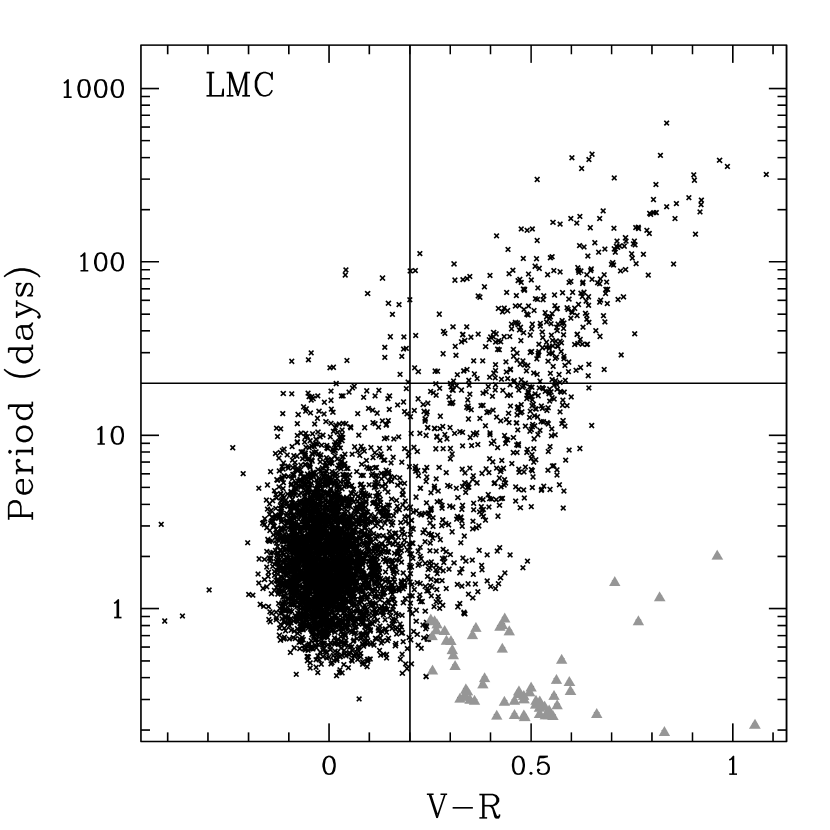
Figure 22: Left Panel: Color Period Diagram for $4634$ EBs in the LMC. The gray filled triangles represent the foreground population. Right Panel: Color Period Diagram for $1508$ EBs in the SMC. The figure shows the higher fraction of long period EBs that belong to the young star region in the SMC than in the LMC.

The Color Period Diagram is shown in the left panel of Figure 22; this diagram clearly shows the young EBs with periods $P\lesssim 20\mathrm{d}$ and a second population ($333$ objects) of long period, evolved EBs with periods $P>20\mathrm{d}$ and $\vr>0.2~{}\mathrm{mag}$. Several interesting features emerge in Figure 22: there is a paucity of long period objects on the young star region of the CMD, and a corresponding lack of short period objects with very red colors. Furthermore, the red ($\vr>0.2~{}\mathrm{mag}$) population shows a positive correlation between period and color. There are virtually no long period, blue objects or short period, red objects in this group. In contrast, the young star region shows no such correlation. This structure in the Color Period Diagram is a consequence of (i) Kepler’s Third Law, (ii) the probability that an EB is favorably oriented in space to allow eclipses to be detected ($\mathrm{Prob}=(R_{1}+R_{2})/a$) where $R_{1}$ and $R_{2}$ are the radii of the primary and secondary stars, respectively and $a$ is the semi major axis, and (iii) that objects usually evolve in this diagram at constant period, from blue to red. Long period binary stars have large semi-major axes. When both stars are on the young star region, their relatively small radii yield a relatively low probability that they will eclipse when seen from our vantage point. When one of the pair evolves away from the young star region, one of these radii (typically $R_{1}$) will increase. The consequence of this is an increase in the probability that eclipses will be detected. This accounts for the presence of red, long period stars and the absence of corresponding young progenitors. The situation is different for short period systems. These are relatively likely to be detected because of their small semi-major axes, and are prominent on the blue side. As one of these stars evolves and expands rapidly, it may engulf the companion and enter a stage of common envelope evolution in which the expanding star overflows the second Lagrangian point $L_{2}$ (Paczynski, 1976); leading to the disappearance of eclipses. Common envelope system differ from contact binaries (Kallrath & Milone, 1999; Hilditch, 2001; Shore, Livio & van den Heuvel, 1994) in which two young stars overflow their first Lagrangian point ($L_{1}$) and their Roche equipotential surface assumes a dumbbell shape. Contact systems usually show ellipsoidal variation and, if the orbital inclination is large enough, also eclipses; EBs of the W UMa type belong to this category. Shore, Livio & van den Heuvel (1994) and Iben & Livio (1993) provide more information on common envelope binaries. The correlation between period and color among red objects reflects the general correlation between radius and color for the evolved partner.

3.2 Foreground objects

The left panel of Figure 22 reveals a population of $\sim 63$ EBs with low periods ($P\lesssim 2\mathrm{d}$) and high color ($\vr>0.3~{}\mathrm{mag}$). These objects are probably foreground galactic EBs composed of late type stars. This interpretation is suggested by several factors. First, due to the large angular extent of the LMC, there is foreground contamination in the LMC MACHO fields (Alcock et al., 2000b); in particular the feature marked “H” in the CMD of their Figure $1$ indicates foreground galactic disk stars and is centered at $\vr\sim 0.5~{}\mathrm{mag}$ as is our presumptive foreground population. Second, both the short period of these EBs, and the shape of their light curves which are either detached or mildly distorted, strongly suggests that the stars making up this population are small, late type stars; this is further borne out by their color, again typical of a solar like star; Finally, the CMD of this population, shown in Figure 23 clearly shows what appears to be a turnoff feature at $\vr\sim 0.4~{}\mathrm{mag}$, with few evolved objects ($\vr>0.7~{}\mathrm{mag}$). It is interesting to note that the overall shape of this population in the Color Period Diagram shows, on a smaller scale, the same features of the LMC diagram; a Main Sequence is clearly visible in Figure 23 and the evolved EBs show the same Color Period correlation of their LMC counterparts in Figure 22.

Figure 23: CMD of the LMC sample (left panel) and of the foreground population (right panel,filled hexagons).

3.3 The Small Magellanic Cloud sample

Figure 24 shows the CMD for $1508$ EBs in the SMC sample out of the $1509$ in the sample; one EB which has valid data only in the $R_{\mathrm{MACHO}}$ band is not shown because it was not possible to determine the standard magnitudes via Eq. 2.7. The general remarks made for the LMC CMD apply here as well and we used a reddening vector with the same inclination as the LMC. The figure clearly shows the young star region which is composed of $1412$ EBs ($94\%$) whereas there are just $96$ evolved EBs. We estimate the SMC reddening from Zaritsky et al. (2002); from their Figure $19$ we infer a mean $A_{V}\sim 0.3~{}\mathrm{mag}$ for their hotter SMC population, relevant to our sample which is composed mostly of early type hot stars on the young star region. We use the same reddening vector as the LMC, $\frac{A_{V}}{E(\vr)}=5$, and find a mean $E(\vr)=0.06~{}\mathrm{mag}$.

Figure 24: CMD for $1508$ EBs in the SMC sample. The reddening vector is $\frac{A_{V}}{E(\vr)}=5$; the adopted values of $\langle A_{V}\rangle$ and $\langle E(\vr)\rangle$ are $0.3~{}\mathrm{mag}$ and $0.06~{}\mathrm{mag}$.

The Color Period Diagram is shown in the right panel of Figure 22; the general considerations made for the LMC Color Period Diagram apply here as well. The diagram shows $5$ EBs with low period ($P<1\mathrm{d}$) and red color ($\vr\sim 0.6~{}\mathrm{mag}$) which are probably foreground objects. The much smaller number of foreground objects in the SMC is probably due both to its smaller angular size and to its higher galactic latitude ($l\sim-44^{\circ}$ compared to $l\sim-33^{\circ}$ for the LMC). We can further test the hypothesis that these two short period, red populations in the LMC and SMC are due to foreground objects by comparing the ratio of their numbers to the ratio of the areas of the LMC and SMC, which we can estimate from Figures 28 and 37; if these objects are indeed foreground these two ratios should be roughly equal. From the figures we can estimate the sky area of the LMC as $\sim 110\Box^{\circ}$ and the sky area of the SMC as $\sim 10\Box^{\circ}$; their ratio is thus similar to the ratio of the numbers of EBs in the two populations as expected.

4 Comparison between the Large Magellanic Cloud and the Small Magellanic Cloud samples

Although the basic features of the CMD and the Color Period Diagram are the same for LMC and SMC, there are some differences, shown by Figure 22 and Table 9.

Table 9: Summary of long period EBs in the SMC and LMC.

Galaxy	Total	Young stars	Evolved	Long Period	Long Period young stars	Long Period evolved stars
LMC	$4634$	$3760(81\%)$	$874(19\%)$	$356$	$23(6\%)$	$333(94\%)$
SMC	$1508$	$1412(94\%)$	$96(6\%)$	$75$	$23(31\%)$	$52(69\%)$

The fraction of blue ($\vr<0.2~{}\mathrm{mag}$) EBs is higher in the SMC than in the LMC. More striking, the fraction of blue long period ($\vr<-0.2~{}\mathrm{mag}$, $P>20\mathrm{d}$) EBs is much higher in the SMC than in the LMC. To further investigate the differences between the two samples we carried out a Kolmogorov-Smirnov (KS) test on the distributions of the absolute magnitudes $M_{V}$ and $M_{R}$, their difference $M_{V}-M_{R}$, and the periods $P$ of the two samples. We adopted a distance modulus of of $18.88$ for the SMC (Dolphin et al., 2001) and $18.5$ for the LMC (van der Marel et al., 2002). Magnitudes and colors were dereddened using $\langle A_{V}\rangle=0.64~{}\mathrm{mag}$, $\langle E(V-R)\rangle=0.128~{}\mathrm{mag}$ for the LMC and $\langle A_{V}\rangle=0.3~{}\mathrm{mag}$, $\langle E(V-R)\rangle=0.06~{}\mathrm{mag}$ for the SMC before subtracting the distance moduli. The Empirical Cumulative Distribution Functions (ECDFs) of these quantities are shown in Figure 25. A KS test confirms that the distributions of $P$ and $M_{V}-M_{R}$ are different at $>99.9\%$ confidence level; for the distributions of $M_{V}$ and $M_{R}$ the KS test gives a probability of $\sim 99.4\%$ and $\sim 98.5\%$ respectively for them being different. The $M_{V}-M_{R}$ plot shows that EBs in the SMC tend to be bluer, not surprising given that a higher percentage of objects belong to the young star CMD region in the SMC than in the LMC. The period distributions show that the SMC EBs have on average shorter periods, again not surprising given the much higher percentage of evolved systems in the LMC than in the SMC and the fact that evolved systems have on average higher periods than the young systems (as shown by the Color Period Diagrams in Figure 22).

Figure 25: ECDFs for the distribution of $M_{V}$ (above left), $M_{R}$ (above right), $M_{V}-M_{R}$ (Below left) and $P$ (below right) for the SMC (continuous line) and the LMC (dashed line).

5 Cross correlation with the OGLE-II samples

The EBs in our samples have been cross correlated with the corresponding OGLE-II samples. Stars in the samples were identified if their right ascension (RA) and declination (DEC) differed by less than $27.2\arcsec$ and if their periods differed by $<1\%$. We used a very large search radius to be conservative. The astrometric precision for both surveys is typically $\sim 1\arcsec$, but a few stars which had much larger differences in RA and/or DEC turned out to be matches upon inspection of their periods: in particular we found in the LMC $32$ matches with a position difference bigger than $10\arcsec$ and $2$ matches with a position difference bigger than $20\arcsec$. However most of the matches were within narrower radii: for the LMC roughly half of the matches ($534$ out of $1236$) were found within of $\sim 2\arcsec$, compatible with the astrometric precision of both MACHO and OGLE surveys; almost all of them ($1019$) were within $\sim 4\arcsec$. We tested the robustness of our method of finding matches by investigating the probability for two periodic objects with a period difference of $<1\%$ to be within $27.2\arcsec$ of each other. To do this we selected a random sample of $5000$ objects out of the $\sim 66000$ periodic ones found by MACHO in the LMC and we counted the frequency of pairs of objects with both periods from the red and the blue lightcurves (as found by Supersmoother) differing by $<1\%$ and positions within $27.2\arcsec$. Most of the matches we found were due to the same object being observed in different tiles and only in one case did we find a possibly genuine match; we thus conclude that the probability of two objects being erroneously classified as a match is $\sim 0.02\%$ and therefore our method of finding matches is robust.

5.1 The Large Magellanic Cloud sample

Our search produced $1236$ matches in the LMC. The MACHO and OGLE-II periods agree to high accuracy as shown in Figure 26; usually much better than the $1\%$ cut we imposed. Histograms of position differences are shown by Figure 27. Both panels show the entire span of the differences; the differences in Right Ascension range from $\sim-20\arcsec$ to $\sim+20\arcsec$ but the left panel shows this range multiplied by the cosine of the declination ($\sim-70^{\circ}$) which gives a range from $\sim-7\arcsec$ to $\sim+6\arcsec$.

Figure 26: Percentage difference for MACHO vs. OGLE-II period for the 1236 OGLE-II matches in the LMC sample.

Figure 27: Left Panel: histogram of the differences between Right Ascensions for $1236$ MACHO OGLE-II matches in the LMC. Right Panel: histogram of the differences between declinations. The bin size is equal to $1/30$ of the range of the differences in both cases.

The sky coverage of the two surveys was different: OGLE-II, from which the sample was derived, covered about $4.5\Box^{\circ}$ in the central region of the LMC whereas the sky coverage of MACHO was larger. Figure 28 shows the positions of the EBs in both catalogues and Figure 29 shows the corresponding MACHO field number; the fields at the center of the LMC are drawn with continuous lines, the ones at the periphery with dashed lines.

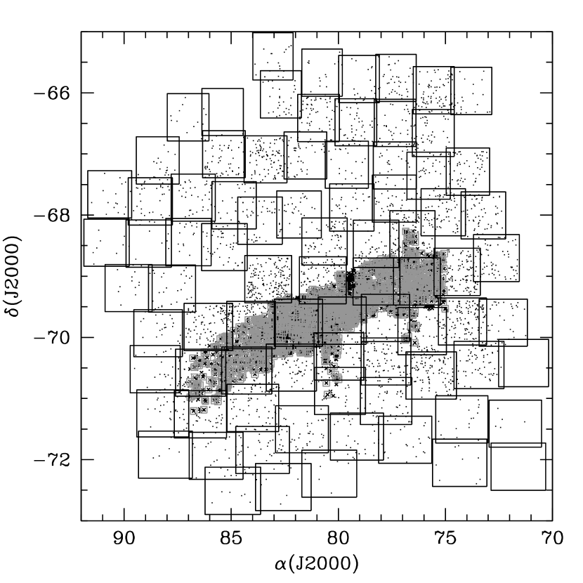
Figure 28: Cross correlation between MACHO and OGLE-II LMC samples: points represent MACHO stars, crosses OGLE stars and gray empty boxes the matches.

Figure 29: MACHO LMC field numbers.

5.2 Comparison between the center and the periphery of the LMC

In view of the different sky coverage of the MACHO and OGLE-II surveys, it is interesting to analyze separately the stars in MACHO fields covering the center of the LMC (which roughly correspond to the OGLE-II sky coverage) and the stars in the MACHO fields at the periphery. Figure. 29 shows that the fields in the center are 1, 2, 3, 5, 6, 7, 8, 10, 11, 12, 13, 14, 15, 18, 19, 47, 77, 78, 79, 80, 81 and 82. There are $2620$ EBs in the center and $2014$ in the periphery. Figure 30 shows the CMD and the Color Period Diagram for the center and the periphery of the LMC respectively; Figure 31 shows the histograms for the magnitudes, the color and the period. The figures reveal several differences between the two samples; to check these we performed a KS test for $V$, $\vr$ and $P$ and found that at high confidence level ($>99.9\%$) the distributions are different. These differences are statistically significant but not large enough to be considered astrophysically important. In particular the difference in period distribution could be attributed to the lower sampling in the outer fields, making it less likely to detect the longer period EBs. The sampling might also be the cause of the periphery having a higher percentage of bright EBs, since these are easier to find with fewer epochs.

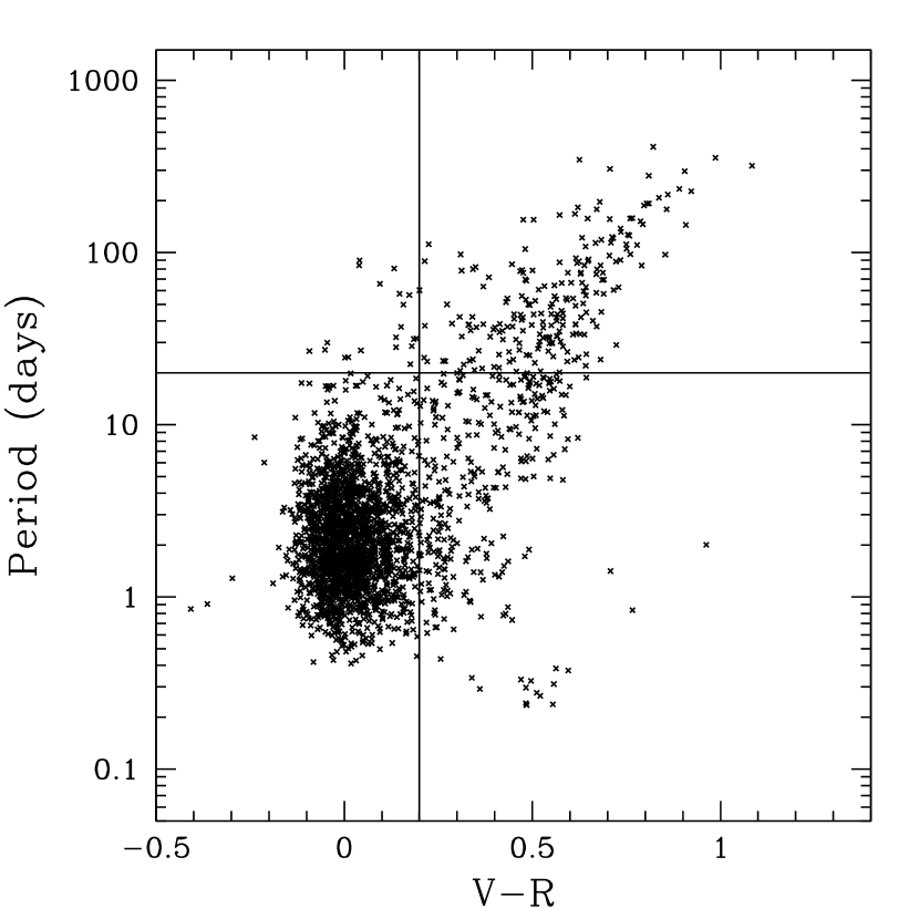
Figure 30: Upper Left Panel: CMD for $2620$ EBs in the center of the LMC. Upper Right panel: CMD for $2014$ EBs at the periphery of the LMC. The CMDs suggest a more continuous transition from the young star region to the evolved star region in the center than in the periphery, especially for $V<19~{}\mathrm{mag}$.
Lower panels: Color Period Diagrams for the same populations. Lower Left Panel: center. Lower Right panel: periphery. The Color Period Diagrams reveal the presence of a long period $(20-100\mathrm{d}$), relatively unevolved ($\vr\sim 0.2~{}\mathrm{mag}$) population in the center but not in the periphery.

Figure 31: Upper Left Panel: Period histogram for $2620$ EBs in the center of the LMC. Upper Right panel: period histogram for $2014$ EBs at the periphery of the LMC. The size of the bins is $\sim 1/100$ of the span of the logarithms of the periods.
Lower panels: Magnitude and Color histograms. Lower Left Panel: center. Lower Right panel: periphery. The bin size is $0.1~{}\mathrm{mag}$ for the $V$ and $R$ histograms and $0.01~{}\mathrm{mag}$ for the $\vr$ one.

5.3 Discussion of OGLE-II MACHO comparison

We finally investigated why we did not find more matches with OGLE-II. The most important reason, we think, is the fact that the techniques employed in assembling the samples are different: the OGLE team built their samples via neural networks (Wyrzykowski et al., 2003, 2004). The two surveys have roughly comparable limiting magnitudes, $V\sim 21.5~{}\mathrm{mag}$; nevertheless we checked how the performance of the two surveys varied with magnitude. We compared the distribution of the $V$ magnitudes for the $2620$ EBs in the central region of the LMC in our sample with those of $1198$ matches and the $1327$ EBs from OGLE-II without MACHO counterparts (these two numbers do not add up to $2580$, the size of the OGLE-II sample, because for some EBs the $V$ magnitude was not reported). The histograms of these three distributions are shown in Figure 32.

Figure 32: $V$ distribution for MACHO $2620$ EBs in the central region of the LMC (continuous line), $1198$ OGLE-II MACHO matches (dashed line), and $1327$ OGLE-II EBs without MACHO counterparts (long dashed line). The figure shows that OGLE-II EBs with MACHO counterparts are on average brighter than the ones without, and the shape of their $V$ distribution more closely resembles the MACHO $V$ distribution. This is confirmed by a KS test.

The figure shows that OGLE-II EBs with MACHO counterparts, peaking at $V\sim 18~{}\mathrm{mag}$ like the MACHO sample, are on average brighter than the ones without MACHO counterparts, which peak at $V\sim 19.5~{}\mathrm{mag}$. The shape of the $V$ distribution of OGLE-II EBs with MACHO counterparts much more closely resembles the MACHO $V$ distribution; a KS test gives a probability of the two distributions being the same of $\sim 46\%$. The distributions of MACHO $V$ and OGLE-II $V$ without MACHO counterparts, as well as those of these two OGLE-II populations are, on the other hand, shown to be different at $>99.9\%$ confidence level. Both distributions vanish at $V\sim 20.5~{}\mathrm{mag}$, showing that their limiting magnitudes are comparable.

We then studied the distributions of the periods: Figure 33 shows that the OGLE-II EBs without MACHO counterparts have on average longer periods than MACHO EBs in the center of the LMC and than OGLE-II EBs with a MACHO counterpart and the difference is statistically significant in both cases; the period distributions of the MACHO EB of the LMC center and of the MACHO OGLE-II matches are statistically different as well. Therefore, OGLE-II finds a higher proportion of fainter objects than MACHO and this does play a role in not finding an higher number of OGLE-II counterparts to our sample.

Figure 33: Period distribution for $2620$ MACHO EBs in the central region of the LMC (continuous line), $1198$ OGLE-MACHO matches (dashed line), and $1327$ OGLE-II EBs without MACHO counterparts (long dashed line). The figure shows that OGLE-II EBs with MACHO counterparts have on average shorter periods than the ones without.

We finally studied the distribution of the MACHO-OGLE matches as a function of $V$. We first counted the number of OGLE-II LMC EBs in the MACHO fields, finding $2517$ of them, out of a total of $2580$; of these $2517$ EBs, $1236$ were the matches described above and $1281$ did not have a MACHO counterpart (this last number is smaller than $1327$, the total number of OGLE EBs without MACHO counterpart, because we are now only considering OGLE EBs in MACHO fields). We then studied the distribution, as a function of $V$, of the OGLE EBs in the MACHO fields that both had and did not have a MACHO counterpart and for which the $V$ magnitude was reported: there were $1198$ of the former and $1267$ of the latter. We finally performed the inverse calculation, by first counting the number of MACHO LMC EBs in the OGLE-II fields and finding $1551$ of them; of these $1225$ had an OGLE-II counterpart and $326$ did not; we studied the distribution of both these populations as a function of $V$. The OGLE-II field boundaries were estimated by taking the coordinates of the most extreme EBs in each OGLE-II field. These findings are summarized in Table 10.

Table 10: MACHO OGLE-II matches.

OGLE-II LMC EBs	$2580$
OGLE-II LMC EBs in MACHO fields	$2517$
OGLE-MACHO matches	$1236$
OGLE-II LMC EBs without MACHO counterpart	$1281$
OGLE-MACHO matches with reported $V$	$1198$
OGLE-II LMC EBs without MACHO counterpart with reported $V$	$1267$
MACHO EBs in OGLE fields	$1551$
MACHO EBs in OGLE fields with OGLE counterpart	$1225$
MACHO EBs in OGLE fields without OGLE counterpart	$326$

The distributions of both the OGLE-II EBs with MACHO counterpart and of the MACHO EBs with OGLE-II counterparts are shown in Figure 34; the figure shows the fraction of matches in magnitude bins of $1~{}\mathrm{mag}$; the bin centers range from $V=20.5~{}\mathrm{mag}$ to $V=12.5~{}\mathrm{mag}$. The error bars are estimated by assuming that the matches in each magnitude bin follow a binomial distribution with probability $p=x/N_{b}$ where $x$ is the number of matches in each magnitude bin and $N_{b}$ is the total number of EBs; the error in the expected fraction of matches is then given by Eq 3; in both distributions of Figure. 34 the error bar for the brightest magnitude bin is not shown since in both cases there is only one match, rendering Eq. 3 meaningless. The figure shows that the fraction of matches increases for brighter magnitudes as expected; the fall at $V=13.5~{}\mathrm{mag}$ in the distribution of OGLE matches is probably due to small number statistic as evidenced by the large error bar.

$$\sigma_{N_{b}}=\frac{\sqrt{p(1-p)N_{b}}}{N_{b}}=\sqrt{\frac{p(1-p)}{N_{b}}}\approx\frac{N_{b}}{N_{b}-1}\sqrt{\frac{\frac{x}{N_{b}}(1-\frac{x}{N_{b}})}{N_{b}}}.$$ (3)

Figure 34: Continuous line: $V$ distribution of the fraction of matches for the OGLE-II LMC EBs in MACHO fields with expected error bars. The magnitude bins are $1~{}\mathrm{mag}$ wide and their centers range from $V=20.5~{}\mathrm{mag}$ to $V=12.5~{}\mathrm{mag}$. Dashed line: $V$ distribution of the fraction of matches for the MACHO LMC EBs in OGLE-II fields.

5.4 The Small Magellanic Cloud sample

The same general considerations apply to the SMC sample: the search, performed with the same criteria as the LMC, produced $698$ matches. Figure 35 shows the percentage difference of the MACHO and OGLE-II periods vs MACHO period for the matches; Figure 36 shows the histogram of the differences in RA and DEC.

Figure 35: Percentage difference for MACHO vs. OGLE-II period for the $698$ OGLE-II matches in the SMC sample.

Figure 36: Left Panel: histogram of the differences between Right Ascensions and for $698$ OGLE matches in the SMC sample. Right Panel: histogram of the differences between declinations.

Unlike the LMC, the sky coverage of the two surveys was approximately the same. Figure 37 shows the positions of the MACHO and OGLE EBs on the sky.

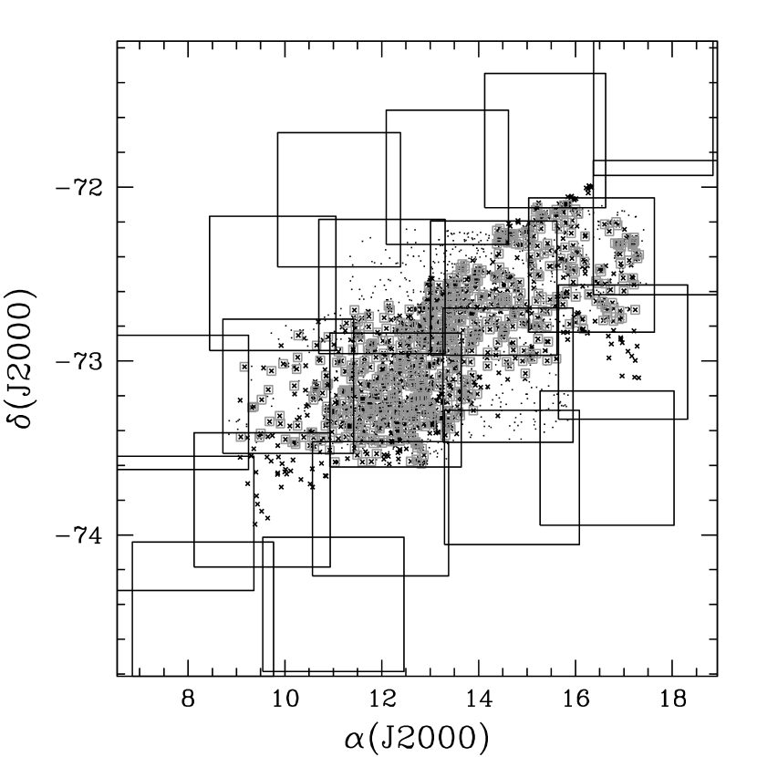
Figure 37: Cross correlation between MACHO and OGLE-II SMC samples: points represent MACHO stars, crosses OGLE stars and gray empty boxes the matches.

We again investigated why we did not find more matches with OGLE-II. Looking at Figure 37 it is evident that one of the reasons is the somewhat different sky coverage of the two surveys (MACHO Fields 207, 208 and 211 are only partially covered by OGLE), but we also looked for other possible explanations. Again, the most likely explanation is the ways in which the samples were assembled, but we also considered the differences in the distributions of magnitudes and periods. As for the LMC, we compared the distribution of the $V$ magnitudes for the $1508$ EBs in our sample which have a valid $V$ with those of $650$ matches and the $666$ EBs from OGLE-II without MACHO counterparts (again these two numbers do not add up to $1351$, the size of the OGLE-II sample, because for some EBs the $V$ magnitude was not reported). The histograms of these three distributions are shown in Figure 38.

Figure 38: Continuous line: $V$ distribution for $1508$ MACHO EBs in the SMC. Dashed line: $V$ distribution for $650$ OGLE-MACHO matches. Long dashed line: $V$ distribution for $666$ OGLE-II EBs without MACHO counterparts. The figure shows that OGLE-II EBs with MACHO counterparts are on average brighter than the ones without, and the shape of their $V$ distribution more closely resembles the MACHO $V$ distribution.

The figure shows that OGLE-II EBs with MACHO counterparts, peaking at $V\sim 17.5~{}\mathrm{mag}$ like the MACHO sample, are on average brighter than the ones without MACHO counterparts, which is more spread out and roughly constant between $18.5~{}\mathrm{mag}<V<16.5~{}\mathrm{mag}$. A KS test shows that these three distributions are different at $>99\%$ confidence level. The behavior at high magnitudes is different for MACHO and OGLE-II: the figure suggests a magnitude limit of $V\sim 21~{}\mathrm{mag}$ for MACHO and $V\sim 20~{}\mathrm{mag}$ for OGLE-II; for $V<19~{}\mathrm{mag}$ MACHO finds many more EBs than OGLE-II.

We then studied the distributions of the periods: Figure 39 shows that OGLE-II EBs with MACHO counterparts have periods that cluster more in the $1\mathrm{d}<P<10\mathrm{d}$ range, as do the MACHO EBs and a KS test gives a probability $\sim 43\%$ for the two distribution to be the same. On the other hand OGLE-II EBs without MACHO counterparts have a larger spread of period values, with more objects having $P>10\mathrm{d}$ and with small “bumps” in the distributions at $\sim 20\mathrm{d}$ and $100\mathrm{d}$ and a KS test shows it to be different from both MACHO and OGLE-II MACHO matches at $>99.9\%$ confidence level. The $V$ distributions of both the OGLE-II EBs without MACHO counterpart and of the MACHO EBs without OGLE-II counterparts are shown if Figure 40; the figure shows the fraction of matches in magnitude bins of $1~{}\mathrm{mag}$ with centers ranging from $V=20.5~{}\mathrm{mag}$ to $V=14.5~{}\mathrm{mag}$; the error bars are estimated again by Eq. 3.

We conclude that differences in sky coverage and in techniques used in assembling the samples, as well as different magnitude limits and in general different behavior at high magnitude of the two surveys all play a role in not finding an higher number of OGLE-II counterparts to our sample; the fact that the SMC was less observed than the LMC by MACHO may also explain why we find fewer long period objects, while the fact that the exposure time for the SMC was double that of the LMC (Alcock et al., 1999) may explain why we find many faint objects.

Figure 39: Continuous line: Period distribution for $1508$ MACHO EBs in the SMC. Dashed line: Period distribution for $650$ OGLE-MACHO matches. Long dashed line: Period distribution for $666$ OGLE-II EBs without MACHO counterparts. The figure shows that both MACHO and OGLE-II EBs with MACHO counterparts have periods that cluster more in the $1\mathrm{d}<P<10\mathrm{d}$ range. OGLE EBs without MACHO counterparts have a larger spread in period and smaller “bumps” in the distribution at $\sim 20\mathrm{d}$ and $100\mathrm{d}$.

Figure 40: Continuous line: $V$ distribution of the fraction of matches of matches for the OGLE-II SMC EBs in MACHO fields with expected error bars. The magnitude bins are $1~{}\mathrm{mag}$ wide and their centers range from $V=20.5~{}\mathrm{mag}$ to $V=13.5~{}\mathrm{mag}$. Dashed line: $V$ distribution of the fraction of matches for the MACHO SMC EBs in OGLE-II fields.

6 The data on line

The data presented in this paper can be accessed on line at the Astronomical Journal website and are mirrored at the Harvard University Initiative in Innovative Computing (IIC) /Time Series Center. At both sites the data consist of a summary table for each Cloud and light curves for all the EBs in the samples. Light curve files contain the unfolded data in MACHO magnitudes; these same files can also be retrieved from the MACHO website. Finally for the LMC, the input and output files used in the JKTEBOP fits are provided.

References

- Alcock at al. (1995) Alcock, C., et al. 1995, AJ, 109, 1653
- Alcock et al. (1996a) Alcock, C., et al. 1996a, AJ, 111, 1146
- Alcock et al. (1996b) Alcock, C., et al. 1996b, ApJ, 470, 583
- Alcock et al. (1997a) Alcock, C., et al. 1997a, AJ, 114, 326
- Alcock et al. (1997b) Alcock, C., et al. 1997b, ApJ, 482, 89
- Alcock et al. (1999) Alcock, C., et al. 1999, PASP, 111, 1539
- Alcock et al. (2000a) Alcock, C., et al. 2000a, ApJ, 542, 281
- Alcock et al. (2000b) Alcock, C., et al. 2000b, AJ, 119, 2194
- Andersen (1991) Andersen, J. 1991, A&A Rev., 3, 91
- Bonanos et al. (2003) Bonanos, A. Z., Stanek, K. Z., Sasselov, D. D., Mochejska, B. J., Macri, L. M., & Kaluzny J. 2003, AJ, 126, 175
- Bonanos (2005) Bonanos, A. Z., 2005, Determining Accurate Distances To Nearby Galaxies, Ph.D. Thesis, Harvard University
- Cook et al. (1995) Cook, K. H. et al. 1995, in ASP Conf. Ser. 83, Astrophysical Applications of Stellar Pulsation, IAU Colloquium 155, ed. R. S. Stobie & P.A. Whitelock (San Francisco: ASP), 221
- Cox (2000) Cox, A. N., 2000, Allen’s Astrophysical Quantities, 4th Ed. (New York: AIP Press; Springer)
- Derekas et al. (2006) Derekas, A., Kiss, L. L., Bedding, T. R., Kjeldsen, H., Lah, P., & Szabó, G. M., 2006, ApJ, 650, L55
- Derekas, Kiss, & Bedding (2007) Derekas, A., Kiss, L. L., & Bedding, T. R., 2007, to appear in ApJ, (astro-ph/0703136)
- Devor (2005) Devor, J., 2005, ApJ, 628, 411
- Dolphin et al. (2001) Dolphin, A. E., Walker, A. R., Hodge, P. W., Mateo, M., Olszewski, E. W., Schommer, R. A., & Suntzeff, N. B., 2001, ApJ, 562, 303
- Etzel (1981) Etzel, P. B., 1981, in Photometric and Spectroscopic Binary Systems, NATO ASI, 111
- Fizpatrick et al. (2002) Fitzpatrick, E. L., Guinan, E. F., DeWarf, L. E., Maloney, F. P. & Massa, D. 2002, ApJ, 564, 260
- Fitzpatrick et. al. (2003) Fitzpatrick, E. L., Ribas, I., Guinan, E. F., Maloney, F. P. & Claret, A. 2003, ApJ, 587, 685
-
Friedman (1984)
Friedman J. H.,
1984,
A Variable Span Smoother.
Technical Report No. 5, Laboratory for Computational Statistics, Department of Statistics, Stanford University - Gaposchkin (1933) Gaposchkin, S. I., 1933, Astron. Nachr., 248, 213
- Gaposchkin (1938) Gaposchkin, S. I., 1938, Harvard Reprint, No. 151
- Gaposchkin (1940) Gaposchkin, S. I., 1940, Harvard Reprint, No. 201
- Groenewegen & Salaris (2001) Groenewegen, M. A. T., & Salaris, M., 2001, A&A, 366, 752
- Grison et al. (1995) Grison, P. et al. 1995, A&AS, 109, 447
- Guinan et al. (1998) Guinan, E. F. et al. 1998, ApJ, 509, L21
- Hilditch (2001) Hilditch, R. W., 2001, An Introduction to Close Binary Stars (Cambridge: Cambridge University Press)
- Iben & Livio (1993) Iben, I, & Livio, M., 1993, PASP, 105, 1373
- Kallrath & Milone (1999) Kallrath, J., & Milone, E. E. 1999, Eclipsing Binary Stars: Modeling and Analysis (New York: Springer)
- Kaluzny et al. (1998) Kaluzny, J., Stanek, K. Z., Krockenberger, M., Sasselov, D. D., Tonry, J. L., & Mateo, M. 1998, AJ, 115, 1016
- Kopal (1939) Kopal, Z., 1939, ApJ, 90, 281
- Kruszewski & Semeniuk (1999) Kruszewski, A., & Semeniuk, I., 1999, Acta Astron., 49, 561
- Lastennet & Valls-Gabaud (2002) Lastennet, E. & Valls-Gabaud, D. 2002, A&A, 396, 551
- Lastennet et al. (2003) Lastennet, E., Fernandes, J, Valls-Gabaud, D. & Oblak, E, 2003, A&A, 409, 611
- van der Marel et al. (2002) van der Marel, R. P., Alves, D. R., Hardy, E., & Suntzeff, N. B., 2002 AJ, 124, 2639
- Metcalfe (1999) Metcalfe, T. S. 1999, AJ, 117, 2503
- Michalska & Pigulski (2005) Michalska, G., & Pigulski, A., 2005, A&A, 434, 98
- Murthy, Kasif & Salzberg (1994) Murthy, S. K., Kasif, S., & Salzberg, S. 1994, Journal of Artificial Intelligence Research, 2, 1
- Nelson & Davis (1972) Nelson, B. & Davis, W. D., 1972, ApJ, 174, 617
- Nelson et al. (2000) Nelson, C. A., Cook, K. H., Popowski, P. & Alves, D. A., 2000, A&A, 119, 1205
- North (2006) North, P., 2006 Ap&SS, 304, 219
- Paczynski (1976) Paczynski, B, 1976, Structure and Evolution of Close Binary Systems, IAU Symposium 73, eds. P. Eggleton, S. Mitton, and J. Whelan (Dordrecht: Reidel), 75
- Pilowski (1936) Pilowski, K., 1936, Zeitschr. Astrophys., 18, 267
- Pojmański (1997) Pojmański, G., 1997, Acta Astron., 47, 467
- Pojmański (2002) Pojmański, G., 2002, Acta Astron., 52, 397
- Popper & Etzel (1981) Popper, D. M. & Etzel, P. B. 1981, AJ, 86, 102
- Protopapas et al. (2006) Protopapas, P., Giammarco, J. M., Faccioli, L., Struble, M. F., Dave, R., & Alcock, C., 2006, MNRAS, 369, 677
- Prša & Zwitter (2005) Prša, A., & Zwitter, T., 2005, ApJ, 628, 426
- Reimann (1994) Reimann J. 1994, Frequency estimation using unevenly-spaced astronomical data Ph.D. Thesis, Department of statistics, University of California, Berkeley
- Ribas et al. (2002) Ribas, I., Fitzpatrick, E. L., Maloney, F. P., Guinan, E. F.,& Udalski, A. 2002, ApJ, 574, 771
- Ribas et al. (2003) Ribas, I., Jordi, C., Vilardell, F., Guinan, E. F., Hilditch, R. W., Fitzpatrick, E. L., Valls-Gabaud, D., & Gimenez, A. 2003, 25th IAU meeting, Properties and Distances of Eclipsing Binaries in M31 Extragalactic Binaries, 25th meeting of the IAU, July 2003, Sydney, Australia
- Ribas & Gimenez (2004) Ribas, I. & Gimenez, A., (eds) 2004, ”Extragalactic Binaries”, New Astronomy Reviews, Vol.48, 647-76
- Ribas et al. (2005) Ribas, I., Jordi, C., Vilardell, F., Fitzpatrick, E. L., Hilditch, R. W. & Guinan, E. F, 2005, ApJ, 635, L37
- Shore, Livio & van den Heuvel (1994) Shore, S. N., Livio, M., & van den Heuvel, E. P. J., 1994, Interacting Binaries (Berlin: Springer)
- Soszyński et al. (2004) Soszyński I. et al., 2004, Acta Astron., 54, 347.
- Stebbins (1911) Stebbins, J., 1911, ApJ, 34, 112
- Southworth, Maxted & Smalley (2004a) Southworth, J., Maxted, P. F. L., & Smalley, B, 2004a, MNRAS, 351, 1277
- Southworth et al. (2004b) Southworth, J., Zucker, S., Maxted, P. F. L., & Smalley, B. 2004b, MNRAS, 355, 986
- Udalski, Kubiak & Szymański (1997) Udalski, A., Kubiak, M., & Szymanski, M., 1997, Acta Astron.47, 319 (OGLE-II)
- Udalski et al. (1998a) Udalski, A, Pietrzyński, G., Woźniak, M, Szymański, M., Kubiak, M.& Żebruń, K. 1998a, ApJ, 509, L25
- Udalski et al. (1998b) Udalski, A., Soszyński, I., Szymański, M., Kubiak, M, Pietrzyński, G., Woźniak, P., & Żebruń, K. 1998b, Acta Astron., 48, 563
- Wilson & Devinney (1971) Wilson, R. E., & Devinney, E. J. 1971, ApJ, 166, 605
- Wilson (1979) Wilson, R. E., 1979, ApJ, 234, 1054
- Wyithe & Wilson (2001) Wyithe, J. S. B. & Wilson, R. E., 2001, ApJ, 559, 260
- Wyithe & Wilson (2002) Wyithe, J. S. B. & Wilson, R. E., 2002, ApJ, 571, 293
- Woolley (1934) Woolley, R.v.d.R., 1934, MNRAS, 94, 713
- Wyrzykowski et al. (2003) Wyrzykowski, Ł., et al. 2003, Acta Astron., 53, 1
- Wyrzykowski et al. (2004) Wyrzykowski, Ł., et al. 2004, Acta Astron., 54, 1
- Zaritsky et al. (2002) Zaritsky, D., Harris, J., Thompson, I. B., Grebel, E. K., & Massey, P., 2002, AJ, 123, 855
- Zaritsky et al. (2004) Zaritsky, D., Harris, J., Thompson, I. B., & Grebel, E. K., 2004, AJ, 128, 1606
- Żebruń et al. (2001) Żebruń et al., 2001, Acta Astron., 51, 317
- Żebruń, Soszyński, & Woz̀niak (2001) Żebruń, K., Soszyński I. & Woz̀niak, P. R. 2001, Acta Astron., 51, 303