Ab initio calculations of the electronic structure of cuprates using large scale cluster techniques

Abstract

The local electronic structures of La₂CuO₄, three members of the Yttrium-family (YBa₂Cu₃O₆, YBa₂Cu₃O₇, and YBa₂Cu₄O₈), and to some extent of Nd₂CuO₄ have been determined using all-electron ab-initio cluster calculations for clusters comprising up to thirteen planar copper atoms associated with their nearest planar and apical oxygen atoms. Spin-polarized calculations in the framework of density functional theory have enabled an estimation of the superexchange couplings $J$. Electric field gradients at the planar copper sites are determined and their dependence on the occupation of the various atomic orbitals are investigated in detail. The changes of the electronic field gradient and of the occupation of orbitals upon doping are studied and discussed. Furthermore, magnetic hyperfine fields are evaluated and disentangled into on-site and transferred contributions, and the chemical shifts at the copper nucleus are calculated. In general the results are in good agreement with values deduced from experiments except for the value of the chemical shift with applied field perpendicular to the CuO₂-plane.

I Introduction

The discovery bib:bednorzmueller of high temperature superconductivity has initiated great experimental and theoretical efforts which aimed at a detailed understanding of these materials. Nevertheless, a generally accepted theory which explains at least the most important properties of the high temperature superconductors could not yet be presented which is possibly related to the complex electronic structures of these materials.

Therefore, very early on ab-initio methods have been employed to determine the electronic properties of these materials. Mostly, band-structure techniques have been employed which are reviewed in Ref. [bib:Pickett, ]. In our contrasting approach to electronic structure calculations, we use cluster techniques in the framework of spin-polarized density functional theory with localized basis functions which are especially well suited for the calculation of local properties.

In particular, the cluster method has been successfully applied to the determination of charge and spin-density distributions in the cuprate plane and to a reasonably accurate evaluation of electric field gradients and magnetic hyperfine fields for planar copper and oxygen nuclei in La₂CuO₄ and YBa₂Cu₃O₇ using clusters comprising five planar copper and their nearest neighboring planar and apical oxygen atoms bib:huesser2000 ; bib:renold2001 .

In this work, these calculations are extended to include clusters representative of La₂CuO₄, YBa₂Cu₃O₆, YBa₂Cu₃O₇, YBa₂Cu₄O₈, and to some extent of Nd₂CuO₄. The development of both hard- and software has led to a significant improvement of the quality of our calculations by use of larger clusters comprising up to thirteen planar copper atoms. This allows a careful study of the convergence of the calculated local properties with respect to the cluster size.

The paper is organized as follows: We will first outline the cluster technique and introduce the used clusters in Sec. II. Sec. III is devoted to a discussion of the spin distribution and contains estimations of exchange couplings in the cuprates. In Sec. IV we report on the calculation of electric field gradients (EFG) at the planar copper sites in the different cuprates. The convergence of the results with respect to the cluster size is demonstrated and the various contributions of the molecular orbitals (MO) and atomic orbitals (AO) to the EFG are elucidated. The calculated distribution of charges and holes reveals that the 3$d_{3z^{2}-r^{2}}$ AO of the copper is not fully occupied. The doping dependence of these distributions and of the EFG are evaluated and compared to nuclear quadrupole resonance data. Sec. V contains a careful examination of hyperfine parameters and their disentanglement into on-site and transferred contributions. Calculations of chemical shieldings are presented in Sec. VI and in particular, the role of the reference substance for magnetic shifts of the copper is discussed. The paper is terminated with the summary and conclusions in Sec. VII.

II The cluster technique

The idea of the cluster technique is to select a contiguous region out of the solid and to treat the electrons therein with standard many-body theories. This so-called core region is surrounded by a shell of basis-free pseudopotentials which prevent the electrons to be attracted by positive point charges and provide smooth boundary conditions. The core and the boundary regions are embedded in a large lattice of background point charges to ensure a very good approximation for the Madelung potential. In the case of the two undoped parent compounds, La₂CuO₄ and YBa₂Cu₃O₆, the values chosen for the background point charges are based on the formal valence of the constituents. In clusters representative of YBa₂Cu₃O₇ and YBa₂Cu₄O₈ the formal valences had to be slightly modified to reach charge neutrality.

The calculations were performed in the framework of spin-polarized density functional theory which provides a good trade-off between accuracy and computational cost. (Hartree-Fock theory, which completely neglects correlation effects, yields poor results. In contrast, configuration interaction methods, which correctly include both exchange and correlation effects in their Hamiltonian, require enormous computer resources and are currently prohibitive for the cluster sizes considered here.) For the representation of the exchange and correlation functionals, the potentials of Becke bib:becke1 ; bib:becke2 and Lee, Yang, and Parr bib:LYP , have been used. All atoms in the core region of the clusters employ the standard triple zeta basis sets (6-311G). For the determination of the ground state of the many-electron system and the evaluation of the observed quantities, the Gaussian03 quantum chemistry software package bib:gaussian03 was used.

It is desirable to have as many atoms as possible in the core region, but the available computer resources and the convergence of the self-consistent field procedure are the limiting factors in this respect. As already mentioned, these limits have been pushed further since our first use of the cluster technique (see Ref. [bib:suter97, ]) which now allows to use larger clusters including up to nearly 1000 electrons.

In this work we present results for clusters comprising 5, 9, and 13 planar copper atoms together with their nearest planar and apical oxygen atoms for clusters representative of La₂CuO₄, YBa₂Cu₃O₆, YBa₂Cu₃O₇, YBa₂Cu₄O₈, and Nd₂CuO₄. In Table 1 the constitutive properties of all the used clusters for every substance are listed. The layout of the CuO₂ plane for the three cluster sizes is displayed in Fig. 2. The lattice constants and the positions of the atoms in the unit cells for the three clusters of the Y-family were chosen according to experimental structure determinations and are taken from Refs. [bib:radaelli1994, ; bib:cava1990, ; bib:bordet1987, ; bib:fischer1989, ]. The buckling of the planar oxygen atoms is not shown in Fig. 2. For La₂CuO₄, the calculations were performed for the tetragonal structure with lattice constants $a=b=3.77$ Å, $c=13.18$ Å and atomic positions according to Ref. [bib:radaelli1994, ].

substance	name	N	P	E	B
	Cu5O26	31	42	395	533
La2CuO4	Cu9O42	51	62	663	897
	Cu13O62	75	78	991	1313
	Cu5O21	26	194	345	468
YBa2Cu3O6	Cu9O33	42	62	473	780
	Cu13O49	62	86	841	1144
	Cu5O21	26	37	345	468
YBa2Cu3O7	Cu9O33	42	62	473	780
	Cu13O49	62	86	841	1144
	Cu5O21	26	37	345	468
YBa2Cu4O8	Cu9O33	42	53	473	780
	Cu13O49	62	73	841	1144

Table 1: Compilation of the used clusters with their constitutive properties. N: number of atoms with a full basis set, P: number of atoms with (basis-free) pseudopotentials, E: number of electrons in the core region, B: number of basis functions.

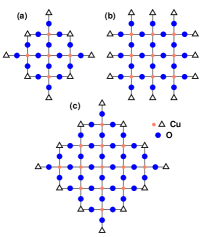
Figure 1: (color online). The layout of the CuO₂ planes in all of the used clusters, (a) with 5 planar copper atoms, (b) with 9 planar copper atoms, and (c) with 13 planar copper atoms. The apical oxygens are not shown. The empty triangles denote Cu²⁺ ions simulated by a pseudopotential.

III Spin distribution

Within the spin-polarized formalism, the spin multiplicity $M$ of a cluster is free parameter of the calculation. In a simple ionic picture, the planar copper and oxygen atoms have a valence of $+2$ and $-2$, respectively. This leads to a $3d^{9}$ configuration for the copper atom with a total spin of one half whereas the oxygen valence gives zero total spin. This suggests two choices of spin multiplicities with a physical significance, a “ferromagnetic” spin multiplicity with all spins parallel and an “antiferromagnetic” spin multiplicity with two neighboring spins being antiparallel. However, other spin multiplicities are also possible leading to spin alignments which can be viewed as superpositions of an antiferromagnetic and a ferromagnetic spin state. We anticipate that the calculated total energy is always lowest for $M$ that corresponds to an antiferromagnetic alignment. In Table 2 the chosen spin multiplicities $M$ are tabulated for each cluster size. The antiferromagnetic (ferromagnetic) spin multiplicities are in bold (normal) face. The superpositions are in parentheses.

cluster	multiplicities
Cu5O26	(2), 4, 6
Cu9O42	2, (4), (6), (8), 10
Cu13O62	(4), 6, (8), (10), (12), 14

Table 2: Chosen spin multiplicities for the different clusters. Numbers in bold face denote multiplicities leading to an “antiferromagnetic” (4, 2, and 6) and a “ferromagnetic” (6, 10, and 14) spin alignment. Note that the possible spin multiplicities are determined solely by the number of planar copper atoms and are therefore independent on the specific material.

In Fig. 2 the spin density along the planar Cu-O bonds is drawn for the large Cu₁₃ cluster representative of YBa₂Cu₃O₆ in the case of $M=14$ corresponding to the ferromagnetic spin alignment (upper panel) and in the case of $M=6$ corresponding to the antiferromagnetic spin alignment (lower panel). The total energy for the latter spin multiplicity is 2.9 eV lower than that of the former. The double humps at the copper positions originate from the approximately singly occupied $3d_{x^{2}-y^{2}}$ atomic orbital. The spins of neighboring coppers are indeed parallel for the ferromagnetic case and antiparallel for the antiferromagnetic case thus confirming the simple physical picture given above. It is important to note that these spin density distributions are obtained also in the smaller clusters and in the other substances considered. A close inspection of the values at the copper sites (upper panel) shows a difference between the three inner coppers and the two coppers at the borders. This is due to the fact that the latter have only one nearest-neighbor (NN) Cu ion which implies a single transferred hyperfine field ($B>0$) whereas the formers have 4 NN leading to 4$B$. This will be further discussed in detail in Sec. V.1.

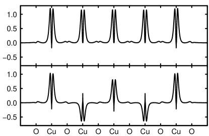
Figure 2: Plot of the spin density along the planar Cu-O bonds in the Cu₁₃ cluster for YBa₂Cu₃O₆. The upper (lower) panel shows the ferromagnetic (antiferromagnetic) spin configuration with $M=14$ ($M=6$).

Furthermore, the ground state energy of the antiferromagnetic spin alignment is consistently lower than that of the ferromagnetic spin alignment. This important feature of our cluster method can be exploited to investigate on the exchange couplings in the different materials.

The Heisenberg Hamiltonian is given by

$$\mathcal{H}=-J\sum_{\langle\>i,j\>\rangle}\mathbf{S}_{i}\cdot\mathbf{S}_{j}$$ (1)

where the summation is restricted to pairs of indices $(i,j)$ with the corresponding sites being nearest neighbored (and with $j>i$ to avoid double counting).

For a given material and cluster size, we can obtain ground state energies $E_{M}$ and ground state wavefunctions $\psi_{M}(\mathbf{r},\sigma)=\phi_{M}(\mathbf{r})\chi_{M}(\sigma)$ for any of the allowed multiplicities $M$ (see Table 2). This is, however, not sufficient for a determination of $J$ since $\langle\>\chi_{M}|\>\sum\mathbf{S}_{i}\cdot\mathbf{S}_{j}\>|\>\chi_{M}\>\rangle$ is in general not easy to determine. However, for a two spin state, the Heisenberg model has an exact solution with $\langle\>\chi_{3}|\>\mathbf{S}_{1}\cdot\mathbf{S}_{2}\>|\>\chi_{3}\>\rangle=3/4$ and $\langle\>\chi_{1}|\>\mathbf{S}_{1}\cdot\mathbf{S}_{2}\>|\>\chi_{1}\>\rangle=-1/4$. This leads to the following idea:

We replace the expectation values of the spin operators in the Heisenberg Hamiltonian by the product of the Mulliken spin densities at the respective lattice sites,

$$\langle\>\chi_{M}|\>\mathbf{S}_{i}\cdot\mathbf{S}_{j}\>|\>\chi_{M}\>\rangle=\rho_{s}^{M}(\textrm{Cu}_{i})\rho_{s}^{M}(\textrm{Cu}_{j}),$$ (2)

with the requirement that in the triplet state of the two-spin system

$$\alpha\rho_{s}^{3}(\textrm{Cu}_{i})\rho_{s}^{3}(\textrm{Cu}_{j})=1$$ (3)

with a reduction factor $\alpha$.

(Note that the name “spin density” might be misleading. It is in fact not a spin density, but an integrated spin density, i.e. a spin. Nevertheless, we persevere with this term which is commonly used in quantum chemistry.) With clusters comprising only two planar copper atoms, we determined $\rho_{s}^{3}(\textrm{Cu}_{i})=0.67$ for both copper sites which yields $\alpha=2.23$. This reduction of the spin density from its value in an ionic model ($\rho_{s}^{3}(\textrm{Cu}_{i})<1$) is due to the fact that also the planar oxygen atoms carry a small amount of spin density. It has nothing to do with the reduction of the mean magnetic moment in the Heisenberg model by quantum fluctuations. We thus arrive at the following modified Heisenberg-type equation for the determination of $J$:

$$E_{M}=-\alpha J\sum_{\langle\>i,j\>\rangle}\rho_{s}^{M}(\textrm{Cu}_{i})\rho_{s}^{M}(\textrm{Cu}_{j})\equiv-\alpha J\Sigma.$$ (4)

In Fig. 3 the ground state energy is plotted versus $\Sigma$ for the different spin multiplicities $M$ in the case of the large Cu₁₃ cluster representative of La₂CuO₄. A straight line with slope $\alpha J=350$ meV can be fitted.

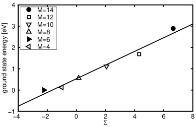
Figure 3: Ground state energy versus $\Sigma$ (see Eq. 4) for all spin multiplicities $M$ of the Cu₁₃ cluster representative of YBa₂Cu₃O₆.

The results of this fit are given in Fig. 4. It is observed that the exchange couplings are fairly independent on the size of the cluster. Furthermore, they are all in the same range of about 150 meV. It is only the optimally doped YBa₂Cu₃O₇ that has a slightly lower exchange coupling which is mainly due to the buckling of the planar oxygens. The two antiferromagnetic substances La₂CuO₄ and YBa₂Cu₃O₆ and the underdoped YBa₂Cu₄O₈ have similar values of $J$.

The calculated antiferromagnetic couplings are in good agreement with data keimer ; shamoto and also with theoretical values munoz obtained from smaller clusters but with more sophisticated ab-initio methods than used here.

We therefore conclude that the antiferromagnetic exchange interactions between two copper neighbors are an intrinsic property of the CuO₂ plane and depend only weakly on the specific material of experiments.

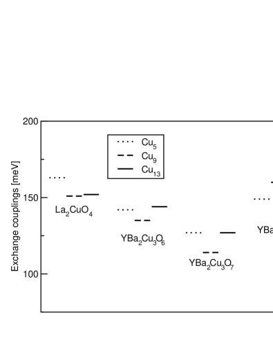
Figure 4: Exchange couplings fitted as described in the text.

IV Electric field gradients

IV.1 Outline

Electric field gradients (EFG) are extremely sensitive to the (non-spherical) charge distributions around the nucleus of interest. In the past twenty years a large quantity of nuclear quadrupole resonance data has been accumulated for high-temperature superconducting cuprate compounds. Of particular interest are the EFGs at the planar copper site and their changes upon doping since they reflect the local charge distribution and provide insight into the population of the different atomic orbitals.

We have already published calculated values for the EFGs in La₂CuO₄, YBa₂Cu₃O₇, and Nd₂CuO₄ obtained for clusters with five copper atoms $(N=5)$ in the plane (see e.g. Refs. [bib:huesser2000, ; bib:renold2001, ]). In this paper we add results for larger clusters ($N=9$ and 13) and report in addition results for YBa₂Cu₃O₆ and YBa₂Cu₄O₈.

In subsection IV.2 we first investigate on the influence of finite size effects. Next (subsection IV.3) a detailed analysis of the contributions to the copper EFG in terms of molecular orbitals is presented. We then postulate in subsection IV.4 an approximate relationship between the copper EFG values and the partial atomic Mulliken charge populations of the orbitals $3d_{x^{2}-y^{2}}$ and $3d_{3z^{2}-r^{2}}$. Although approximate within about 10 % only, this provides insight into the EFG differences observed in different compounds as well as their changes upon electron or hole doping. The latter relationship is discussed in subsection IV.6.

In subsection IV.7 the theoretical results are compared to experimental data and an extended discussion about the interpretation of the results is presented.

IV.2 Dependence of the calculated Cu EFG on the cluster size

In Fig. 5 we present the main component $V_{zz}$ of the EFG obtained for the copper in the center of clusters comprising $N$ = 5, 9, and 13 planar copper atoms simulating the La₂CuO₄,  YBa₂Cu₄O₈,  YBa₂Cu₃O₆, and Nd₂CuO₄ compounds. These values have been calculated for spin multiplicity $M$ = 4, 2, and 6, respectively, which correspond to an antiferromagnetic alignment of the spins and yield the lowest total energy. The values for $N$ = 9 and 13 are nearly equal while those for $N$ = 5 are about 10 % to 20 % smaller due to finite size effects. We note that the EFG values for the YBa₂Cu₃O₇ compounds exhibit the same size dependence with values for YBa₂Cu₃O₇ between the those for La₂CuO₄  and YBa₂Cu₃O₆ (see subsection IV.6).

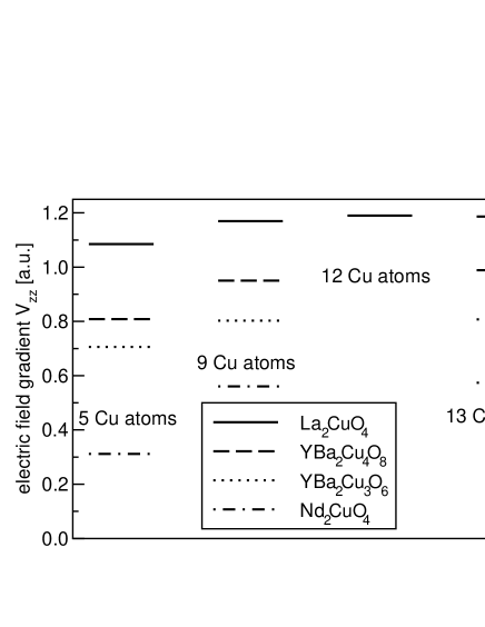
Figure 5: EFG value $V_{zz}$ as a function of the number of Cu atoms in the clusters.

In addition, we have calculated the EFG value for a La₂CuO₄ cluster with an even number ($N$ = 12) of copper atoms without spin polarization (singlet state with $M$ = 1). As seen in Fig. 5 this value is very close to those calculated for $M$ = 9 and 13.

We further note that $V_{zz}$ is given in atomic units (1 a.u. corresponds to 9.71525 $\times$ 10²¹ V m^-2). A comparison to experiments will be made in subsection IV.7.

IV.3 Detailed analysis of contributions

In this subsection we first analyze the various contributions to the copper EFG in detail. It will be shown that the values of the EFG are not solely determined by the occupancies of the $3d_{x^{2}-y^{2}}$ atomic orbital as is often assumed in simplistic models.

The charge distribution is determined by the occupied MOs. The $m^{th}$ MO is represented as a linear combination footnote

$$\phi_{m}(\vec{r})=\sum_{K=1}^{n}\phi_{m}^{K}(\vec{r}-\vec{R}_{K})=\sum_{K=1}^{n}\sum_{k=1}^{n_{K}}c_{m}^{K,k}B_{K,k}(\vec{r}-\vec{R}_{K})$$ (5)

of $n_{K}$ atomic basis functions $B_{K,k}$ centered at the nuclear sites $K=1,\dots,n$, and the $c_{m}^{K,k}$ are the MO coefficients. We assume in the following that the target nucleus $K_{T}$ is at $\vec{R}_{K_{T}}=0$. The contribution of the MO $\phi_{m}$ to the EFG at $K_{T}$ is given by the matrix element

$$V^{(m)}_{ij}=\langle\>\phi_{m}(\vec{r})|\>\frac{3x^{i}x^{j}-r^{2}\delta^{ij}}{r^{5}}\>|\>\phi_{m}(\vec{r})\>\rangle$$

$$=\sum_{K=1}^{n}\sum_{L=1}^{n}\sum_{k=1}^{n_{K}}\sum_{l=1}^{n_{L}}c_{m}^{K,k}c_{m}^{L,l}\times$$

$$\times\langle\>B_{K,k}(\vec{r}-\vec{R}_{K})|\>\frac{3x^{i}x^{j}-r^{2}\delta^{ij}}{r^{5}}\>|\>B_{L,l}(\vec{r}-\vec{R}_{L})\>\rangle.$$ (6)

This matrix element contains contributions from basis functions centered at two nuclear sites $K$ and $L$. Thus we can identify three types of contributions: $(i)$ on-site terms from basis functions centered at the target nucleus ($K=L=K_{T}$, contribution I), $(ii)$ mixed on-site off-site contributions (II), and $(iii)$ purely off-site terms with $K\neq K_{T}$ and $L\neq K_{T}$ (III).

In addition, there is a contribution coming from all nuclear charges $Z_{K}$ and all point charges mentioned in Sec. II which we denote by

$$W_{ij}^{\rm tot}=W_{ij}+W_{ij}^{\rm pc}$$ (7)

where W_ij refers to nuclei in the core region of the cluster and $W_{ij}^{\rm pc}$ to the point charges outside this core. The charges of the bare nuclei at sites $K\neq K_{T}$ in the core are screened by the matrix elements of contribution III with $K=L\neq K_{T}$. Therefore the combined contributions from III and the nuclei (W_ij) are small. The partitioning of the contributions to the EFG tensor $V_{ij}$ thus reads

$$V_{ij}={{}^{I}V_{ij}}+{{}^{II}V_{ij}}+{{}^{III}V_{ij}}+W_{ij}+W_{ij}^{\rm pc}.$$ (8)

More details about these regional partitions can be found in Ref. [bib:stoll, ].

In Table 3 the contributions to the EFG component V_zz for the copper in the center of the Cu₁₃ clusters representative for Nd₂CuO₄, YBa₂Cu₃O₇, and La₂CuO₄ are collected. As expected, the values from region III and W as well as those from point charges outside the core region are small. However, mixed on-site off-site contributions (region II) are substantial. They are mainly transferred via the on-site 3$d_{3z^{2}-r^{2}}$ orbital which has a non-negligible overlap with the 2$p_{z}$ orbitals of the four surrounding planar oxygens. The on-site terms (region I) contain values which come from terms in the evaluation of matrix elements (IV.3) where one basis function is $s$ like and the other $d$ like. Their contribution is denoted by R in Table V. Also the contributions from the Cu $p$ type orbitals are substantial due to the large $\langle\>r^{-3}\>\rangle$ values. The occupancies of the three $d$ orbitals with t_2g symmetry are close to 2 so that their combined contribution to $V_{zz}$ is small. As expected, the distinguished AO is the $3d_{x^{2}-y^{2}}$ with a polarization of 70 % accompanied with smaller but still significant polarization in the orbital $3d_{3z^{2}-r^{2}}$.

IV.4 Model

As pointed out above, a rigorous explanation for the variation of the copper EFG values in different cuprates is very complicated. A simple explanation, however, which concentrates on the two most relevant orbitals, is given in this subsection.

Previously, we have investigated in Refs. [bib:stoll1, ; bib:bersier, ] the changes of the copper EFG values that occur upon doping in La₂CuO₄ and in Nd₂CuO₄. We found that it is sufficient to concentrate on those MOs which contain partially occupied $3d_{x^{2}-y^{2}}$ and $3d_{3z^{2}-r^{2}}$ AOs at the target nucleus. The EFG is then given by

$$V_{zz}=S+\frac{4}{7}\left[N_{3z^{2}-r^{2}}\langle r^{-3}\rangle_{3z^{2}-r^{2}}-N_{x^{2}-y^{2}}\langle r^{-3}\rangle_{x^{2}-y^{2}}\right]$$ (9)

where $S$ is the contribution from all other orbitals and regional partitions. The values for $\langle r^{-3}\rangle$ calculated for the different 3$d$ atomic orbitals are almost identical (e.g. $\langle r^{-3}\rangle_{3z^{2}-r^{2}}=8.004$ a.u. and $\langle r^{-3}\rangle_{x^{2}-y^{2}}=8.042$ a.u.) and therefore are replaced by the average $<r^{-3}>=8.020$ a.u.. We further note that the partial occupation numbers $N$ of the AOs are very similar to the partial Mulliken populations $p_{c}$ which are gathered in Table 4. In particular, the differences

$$\Delta_{d}=p_{c}(3d_{3z^{2}-r^{2}})-p_{c}(3d_{x^{2}-y^{2}})$$ (10)

and

$$N_{3z^{2}-r^{2}}-N_{x^{2}-y^{2}}$$ (11)

are very similar. In Fig. 6 we therefore plot the calculated copper EFG component $V_{zz}$ versus $\Delta_{d}$. The straight line corresponds to

$$V_{zz}=-2.74+7.63\Delta_{d}$$ (12)

which emphasizes the quality of the model.

Table 3: Contributions to the EFG component $V_{zz}$ for the copper in the center of the Cu₁₃ clusters representative for Nd₂CuO₄, YBa₂Cu₃O₇ and La₂CuO₄.

	Nd2CuO4	YBa2Cu3O7	La2CuO4
Wpc	$-0.033$	0.021	0.019
I
R	0.755	0.640	0.474
p	$-1.431$	$-1.157$	$-1.250$
d${}_{x^{2}-y^{2}}$	$-6.378$	$-6.344$	$-6.263$
dxy+dxz+dyz	$-0.072$	$-0.141$	$-0.090$
d${}_{3z^{2}-r^{2}}$	8.309	8.630	8.736
II
s	$-0.003$	$-0.004$	0.004
p	$0.013$	0.014	0.022
d${}_{x^{2}-y^{2}}$	$-0.021$	$-0.020$	$-0.019$
dxy+dxz+dyz	$0.001$	0.001	0.002
d${}_{3z^{2}-r^{2}}$	$-0.585$	$-0.515$	$-3.382$
III + Nuclei	$-0.015$	$-0.061$	$-0.053$
Total	0.538	1.066	1.202

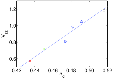
Figure 6: (color online). Theoretical EFG component $V_{zz}$ versus $\Delta_{d}$=$p_{c}$(3d${}_{3z^{2}-r^{2}}$)$-p_{c}$(3d${}_{x^{2}-y^{2}}$) for La₂CuO₄ (black square), YBa₂Cu₃O₇ (blue triangle up), YBa₂Cu₄O₈ (blue triangle down), YBa₂Cu₃O₆ (blue triangle right), Sr₂CuO₂Cl₂ (from Ref [bersier2002, ]) (green circle), and Nd₂CuO₄ (red diamond). The straight line is a fit $V_{zz}=7.63\cdot\Delta_{d}-2.74$.

Table 4: Partial occupation numbers $N$ and partial Mulliken populations $p_{c}$ for the frontier orbitals $3d_{x^{2}-y^{2}}$ and $3d_{3z^{2}-r^{2}}$.

	Nd2CuO4	YBa2Cu3O7	La2CuO4
$N(x^{2}-y^{2})$	1.379	1.375	1.363
$p_{c}(x^{2}-y^{2})$	1.430	1.423	1.406
$N(3z^{2}-r^{2})$	1.820	1.898	1.910
$p_{c}(3z^{2}-r^{2})$	1.865	1.914	1.922

IV.5 Charge and hole distribution and qualitative discussion of bonding

The atomic Mulliken charges $\rho$ for the central copper and neighboring oxygen atom in La₂CuO₄ as calculated for the Cu₁₃ with spin multiplicity $M=6$ are

$$\rho_{0}({\rm Cu})=1.143,\rho_{0}({\rm O}_{p})=-1.635,\rho_{0}({\rm O}_{a})=-1.945.$$ (13)

The corresponding values for the four units surrounding the central one are

$$\rho_{1}({\rm Cu})=1.131,\rho_{1}({\rm O}_{p})=-1.629,\rho_{1}({\rm O}_{a})=-1.944.$$ (14)

while those of units at the boundary of the core region differ at most by one percent due to finite size effects.

We define

$$\rho_{0}(3)=\rho(Cu)+2\rho(O_{p})+2\rho(O_{a})+6$$ (15)

where 6 accounts for the charges of the two La ions in the unit cell. We obtain $\rho_{0}(3)=-0.012$ that is close to zero which emphasizes the suitability of these clusters to represent the local conditions of atoms in the crystal. This point cannot be overstressed since it also means that there is now also confidence in the partial Mulliken populations of the individual orbitals which have been studied in detail elsewhere [bib:stoll2, ].

The partial Mulliken populations of those AO which differ from 2 by more than 0.02 are given in Table 5 and are visualized in Fig. 7 where the area in yellow (gray on top) accounts for an intrinsic hole of 1.5 missing electrons which is compensated by the occupancy of the 4$s$ orbital. All attempts to deduce the distribution of holes which do not take into account the $4s$ orbital are very questionable and misleading.

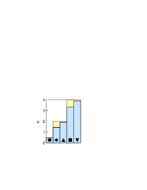
Figure 7: (color online). Partial Mulliken populations of the atomic orbitals (tinted in darker gray (blue)) for La₂CuO₄: Black symbols denote $4s$ (circles), $3d_{x^{2}-y^{2}}$ (diamonds), and $3d_{3z^{2}-r^{2}}$ (triangles up), 2 $\times$ $p($O${}_{p}(2p_{\sigma}))$ for the planar oxygens (squares), and 2 $\times$ $p($O${}_{a}(2p_{z}))$ for the apical oxygens (triangles down). The light gray (yellow) tinted areas denote the missing charge against the simple ionic model.

Table 5: Partial Mulliken populations $p_{c}$ of the AOs in the central unit of La₂CuO₄.

AOs	3$d_{x^{2}-y^{2}}$	3$d_{3z^{2}-r^{2}}$	4$s$	2$p_{\sigma}(O_{p})$	2$p_{z}(O_{a})$
$p_{c}$	1.406	1.922	0.491	1.662	1.946

The ionic picture which assigns charges of +3(La), +2(Sr), +2(Cu), and $-2$(O), respectively is a reasonable approximation for the out-of-plane La- and apical O_a-atoms. The copper and the planar oxygen atoms, however, are rather covalently bound and the relation between charge and hole transfer is not trivial. A Mulliken charge population analysis [bib:stoll2, ] attributes a charge of 1.16 to the copper and $-1.64$ to the planar oxygens but 40% of the hole is transferred to the oxygens leaving 60% on the copper. Since a hole transfer is accompanied by an electron charge transfer in the opposite direction it is concluded that of the total of 0.84 electrons transferred from the oxygen to the copper, 0.40 electrons are accounted for the hole transfer. The remaining 0.44 electrons almost correspond exactly to the Mulliken 4s orbital population. The discrepancy of 0.05 electrons can be attributed to secondary interactions which also involve the 3$d_{3z^{2}-r^{2}}$ and the 2$p_{z}$ apical oxygen orbitals. The substantial occupation of the Cu 4$s$ orbital is responsible for the existence of the hyperfine field transferred from the four next nearest copper atoms which is revealed by NMR experiments.

IV.6 Doping dependence

The measured copper quadrupole frequencies generally increase with hole doping. In particular, in La_2-xSr_xCuO₄, the slope of this increase is reported in bib:japaner ; bib:imai1993 ; bib:haase to be in the range of 0.56$x$ to 0.7$x$. It is of utmost interest to deduce the redistribution of charges that occurs upon doping from these data. This is, however, a complex task because the doped holes will also change the lattice parameters and atomic positions in the unit cell which in turn influence the EFG.

Ab-initio calculations of doping-induced charge redistribution have been reported by Ambrosch-Draxl et al. [Ambrosch, ] for the compound HgBa₂CuO_4+δ. They employed the full-potential linearized augmented plane-wave method and used a series of supercells containing one excess oxygen atom. In principle, total-energy and atomic-force calculations can also be performed for small clusters. They are not feasible, however, for large clusters. We therefore report in the following on investigations of doping dependence with lattice parameters and atomic positions kept fixed at values corresponding to the undoped compound La₂CuO₄. The results are therefore only reliable for small doping, i.e. they should be considered to describe the (linear) slope of changes around the undoped material. We will turn back to changes in the atomic positions at the end of this subsection.

The method of cluster calculations would also enable the study of changes in the local electronic structure that occur by replacing e.g. a trivalent La by a bivalent Sr. These inhomogeneous changes, however, are not the subject of the present investigation where we simulate the long range effects of doping (delocalized holes or electrons) by two different approaches. First we introduce additional point charges at the periphery of the cluster to place an electric field across the cluster to move charges toward or away from the atoms of interest in the cluster center. In this so called “peripheral charges method”, the added system of charges has no physical interpretation except that it can be continuously altered so that charge can be progressively directed to or extracted from important ions of interest in the cluster. The cluster and the system of charges in total keep the same number of electrons and spins but, using for instance a Mulliken population analysis approach, the charge of the cluster center can be progressively changed in a manner expected by doping. In the second approach of simulating doping we have added or removed two electrons from the cluster and repeated the calculation. Changing the number of electrons by an even number allows us to keep the spin state.

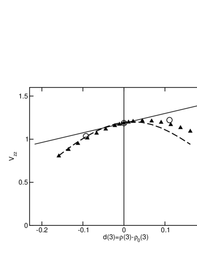
Figure 8: $V_{zz}$ versus ”doping level” $d(3)=\rho(3)-\rho_{0}(3)$ for La₂CuO₄.

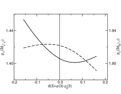
Figure 9: $p_{c}(3d_{x^{2}-y^{2}})$ (solid curve) and $p_{c}(3d_{3z^{2}-r^{2}})$ (dashed curve) versus ”doping level” $d(3)=\rho(3)-\rho_{0}(3)$ for La₂CuO₄.

To discuss the EFGs for doped La₂CuO₄ we define

$$\rho(3)=\rho({\rm Cu})+2\rho({\rm O}_{p})+2\rho({\rm O}_{a})+2\rho({\rm La}),$$ (16)

where the Mulliken charges refer to the central unit and $\rho({\rm La})=3$.

For the undoped Cu₁₃ cluster with spin multiplicity $M$=6 we obtain $\rho_{0}(3)=-0.012$ as discussed above. In Fig. 8 we plotted the EFG component $V_{zz}$ for the central copper versus the doping level $d(3)=\rho(3)-\rho_{0}(3)$. Note that negative values of $d$ would apply to electron-doped materials which for the present case of La₂CuO₄ is of course of no experimental relevance. The two circles at $d=-0.09$ and $d=0.11$ have been obtained by adding and subtracting two electrons, respectively. The triangles denote results obtained with the peripheral charge method [bib:stoll1, ]. All values have been calculated for multiplicity $M$=6.

The slope of the increase of $V_{zz}$ at $d=0$ is 1.12. An analysis of the populations of the frontier orbitals is shown in Fig. 9. For small $d(3)$ but with increasing (hole) doping $p_{c}(3d_{3z^{2}-r^{2}})$ is increased but reaches a maximum at $d(3)=-0.056$ while $p_{c}(3d_{x^{2}-y^{2}})$ is decreased and has a minimum at 0.066. Using Eqs. (9), (10) and (12), the dashed line in Fig. 8 shows the calculated $V_{zz}$.

An analysis of the charges in the occupancies upon doping exhibits that an additional extrinsic hole goes to 15 % to the 3$d_{x^{2}-y^{2}}$ AO, to $2\times 18.7\,\%=37.4\,\%$ to the two O_p $2p_{\sigma}$ AO, to 7 % to the 3$d_{3z^{2}-r^{2}}$ AO and to $2\times 18.7\,\%=37.4\,\%$ to the two O_a $2p_{z}$ AO, while the $4s$ remains practically constant.

It is instructive to compare these results with those obtained in Ref. [Ambrosch, ] for HgBa₂CuO_4+δ. Although the calculational procedures are quite different the essential conclusions are the same. We first define

$$\rho(2)=\rho(3d_{x^{2}-y^{2}})+2\rho(2p_{\sigma})$$ (17)

as the charge of the planar orbitals and correspondingly $d(2)=\rho(2)-\rho_{0}(2)$ as the derivation from the undoped case. We get

$$\rho(2)=0.52\,\rho(3)$$ (18)

which is to be compared with $\rho(2)=0.55\,\rho(3)$ in Ref. [Ambrosch, ]. Thus in both cases the removal of an electron by a dopant atom in the intra-layer induces only half a hole in the CuO₂ plane. The calculated changes of the occupancies of the individual orbitals are somewhat different. For HgBa₂CuO_4+δ a decrease of 35 % for $p_{c}(3d_{x^{2}-y^{2}})$ was reported whereas our value for La₂Cu₃O₄ is 15 %. This is compensated by a smaller decrease of 20 % for $2\times p_{c}(2p_{\sigma})$ compared to 37 %. These differences are, however, of not too much relevance since the assignment of the charge to AO in covalent bonds is anyhow somewhat arbitrary. The turn-over of $V_{zz}$ in Fig. 8 and in the occupancies in Fig. 9 may well be an artefact of the not appropriately adjusted changes in the atomic positions. It should be pointed out, however, that in the calculations of Ambrosch-Draxl et al. [Ambrosch, ] where these positions have been adjusted, the initially linear changes stop at a doping concentration $d(3)=0.22$ and remain constant at higher $d(3)$ values which indicates a saturation of the planar hole content at 0.12.

The essential question now is whether these theoretically predicted redistributions of charges can be corroborated by experimental facts. The slope of increase of $V_{zz}$ of 1.1 is too large compared to the data. We may explain this partially with arguing that the lattice parameter $a$ shrinks upon doping. While it is not feasible to determine the ground-state energy of all atoms with cluster calculations, it is straightforward to study the changes if a single parameter is varied and the results are reliable since relative changes are involved. We have previously reported bib:renold2003a on the changes that occur when the lattice parameter $a$ for a cluster representative of La₂CuO₄ with 5 atoms is varied and found that when $a$ shrinks by 1 % the EFG value $V_{zz}$ is reduced by $\approx 10.7$ %. Assuming a reduction of $a$ by 4 % upon doping, according to data presented in Ref. [bib:bozin, ], we get a reduced slope of $V_{zz}$ of $1.12-0.43=0.69$, which is (very) close to the experimental value. Notice, however, that this argumentation neglects the variation of $V_{zz}$ due to small changes of the positions of the atoms in the $c$-direction, in particular those of the apex oxygen and of the La ions.

IV.7 Comparison with NQR experiments

For a nuclear spin 3/2, the connection between NQR frequencies ${}^{63}\nu_{Q}$ and the main component $V_{zz}$ of field gradients in the case of axial symmetry is given byslichter :

$${}^{63}\nu_{Q}=\frac{\Delta E(\pm 3/2\rightarrow\pm 1/2)}{h}=\frac{e\ ^{63}QV_{zz}}{2h}$$ (19)

with ${}^{63}Q$ being the nuclear quadrupole moment. Unfortunately, directly measured values for ${}^{63}Q$ are not available. The commonly used value of ${}^{63}Q=-0.211\pm 0.004$ b was obtained some time ago by Sternheimerbib:pyykkoe2001 by interpreting excitation spectra with the Hartree-Fock approximation.

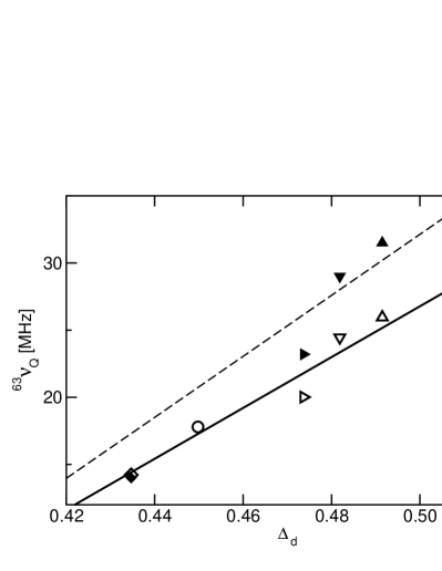
Figure 10: Experimental (full symbols) and calculated (open symbols) quadrupole frequencies ${}^{63}\nu_{Q}$ as a function of the calculated difference of the Mulliken populations $\Delta_{d}$. The symbols denote: La₂CuO₄ (square), YBa₂Cu₃O₇ (triangle up), YBa₂Cu₄O₈ (triangle down), YBa₂Cu₃O₆ (triangle right), Sr₂CuO₂Cl₂ (from Ref [bersier2002, ]) (circle), and Nd₂CuO₄ (diamond).

In Fig. 10 we plot our theoretical values for the quadrupolar frequency ${}^{63}\nu_{Q}$ obtained from the calculated values $V_{zz}$ with the above mentioned value for ${}^{63}Q$ versus the calculated difference of the Mulliken populations $\Delta_{d}$. The straight line corresponds to

$${}^{63}\nu_{Q}=\alpha+\beta\Delta_{d},\,\alpha=-73\,\,\rm{MHz},\,\beta=200\,\,\rm{MHz}.$$ (20)

In the same figure we include data obtained from the various materials plotting them at the corresponding theoretical values $\Delta_{d}$. The experimental values for ${}^{63}\nu_{Q}$ are very accurate but there is of course an uncertainty in the calculated $\Delta_{d}$. Furthermore, we expect the theoretical values for $V_{zz}$ to be less reliable for small $V_{zz}$ due to the cancellations of the various contributions shown in IV.3. The more reliable calculations for the compounds with large $V_{zz}$ (La₂CuO₄, YBa₂Cu₃O₇ and YBa₂Cu₄O₈) systematically predict quadrupole frequencies that are about 15 % lower than the experimental ones. The dashed straight line corresponds to

$${}^{63}\nu_{Q}=\tilde{\alpha}+\tilde{\beta}\Delta_{d}=f(\alpha+\beta\Delta_{d}).$$ (21)

with $f=1.2=1/0.83$. This disagreement between calculations and experiments could be due to a systematic error in the theoretical determination of $V_{zz}$ or due to a higher value of ${}^{63}Q$ than assumed or due to both.

It should also be noted that the NQR frequencies ${}^{63}\nu_{Q}$ depend on temperature as has been reported in detail by Matsumura et al. [matsumura, ] for La₂CuO₄. According to the cluster calculations with variable lattice parameter $a$ (see IV F) the general increase of ${}^{63}V_{zz}$ with temperature in the paramagnetic region is mainly due to the lattice expansion.

Owing to the orthorhombic structure, the EFG at the planar Cu(2) is not axially symmetric in the compounds YBa₂Cu₃O₇ and YBa₂Cu₄O₈ but shows a slight anisotropy since $V_{xx}\neq V_{yy}$. The calculated anisotropy parameters $\eta=|V_{xx}-V_{yy}|/|V_{zz}|$ are $\eta=0.047$ and 0.035, respectively.

The experimentally observed anisotropies have been reviewed by BrinkmannBrinkmann . For the planar copper nuclei, they are somewhat smaller than our theoretical values. Of more importance, however, are the large $\eta$ values (slightly below 1) measured for the chain copper, Cu(1), which are quite unexpected since Cu(1) is not at a crystallographic position that would imply $\eta=1$ by symmetry arguments. An evaluation of the EFG at Cu(1) by cluster methods requires that at least the two nearest neighboring planar copper atoms in the CuO₂-planes above and below the Cu(1) site are considered. We have previously performed bib:huesser1998 ; bib:renold2001 such calculations for a Cu₃O₁₂ cluster representative of YBa₂Cu₃O₇. The calculated bib:renold2001 EFG values for Cu(1) are $V_{xx}=0.601$, $V_{yy}=-0.603$ and $V_{zz}=-0.002$ a.u. which should be compared with the experimental ones $V_{xx}=0.767$, $V_{yy}=-0.773$ and $V_{zz}=0.006$ a.u. as obtained from the measured frequencies with the above mentioned quadrupole moment ${}^{63}Q$. The theoretical values produce an asymmetry parameter in complete agreement with the data whereas the absolute value are again about 20 % smaller than the measured ones.

Recently, Kanigel and KerenKanigelKeren have reported NMR measurements for a series of fully enriched (Ca_0.1La_0.9)(Ba_1.65La_0.35)Cu₃O_y powder samples where doping can vary across the full range from the very underdoped to the extreme overdoped. They determined the nuclear quadrupole frequency from the four peaks of the powder spectra and obtained a convex curve of $\nu_{Q}$ versus doping level which looks very similar to the one (triangles) shown in Fig. 8. They used then also a simulation program to account for asymmetric peaks which provides an increase of $\nu_{Q}$ with doping in the underdoped region but a saturation at the overdoped site.

V Magnetic hyperfine fields

V.1 Theoretical determination

The hyperfine spin Hamiltonians for copper and oxygen nuclei in the CuO₂ planes of the cuprates are given by:

$${}^{63}H^{\textit{\footnotesize{hf}}}_{i}=\mathbf{I}_{i}\cdot\mathbb{A}\cdot\mathbf{S}_{i}+\sum_{j\in NN}\mathbf{I}_{i}\cdot\mathbb{B}\cdot\mathbf{S}_{j}$$ (22)

and

$${}^{17}H^{\textit{\footnotesize{hf}}}_{i}=\sum_{j\in NN}\mathbf{I}_{i}\cdot\mathbb{C}\cdot\mathbf{S}_{j}.$$ (23)

For copper, the hyperfine interaction contains an anisotropic on-site term, $\mathbb{A}$, and a transferred term, $\mathbb{B}$, from the four nearest copper neighbors, which is usually taken to be isotropic, since it is assumed to consist only of a contact term. We will, however, retain the tensorial notation of the transferred field, since we will also be able to calculate a dipolar part of the transferred interaction. For oxygen, the hyperfine interaction $\mathbb{C}$ is with the two nearest copper neighbors.

We have already demonstrated in Refs. [bib:huesser2000, ; bib:renold2001, ] that for La₂CuO₄ and YBa₂Cu₃O₇ it is justified to neglect transferred interactions from further distant copper neighbors, both in the case of copper and oxygen.

On a first-principles level, the hyperfine interactions are basically well known, they consist of an isotropic hyperfine density, $D$, a dipolar interaction, $T^{ij}$, and a spin-orbit interaction term. The core polarization is given by the spin density at the nuclear site $R$ and is evaluated as follows:

$$D(\mathbf{R})=\frac{8\pi}{3}(\rho^{\uparrow}(\mathbf{R})-\rho^{\downarrow}(\mathbf{R})).$$ (24)

If it mainly originates from singly occupied $s$-electrons, it is called Fermi contact. In contrast, if it is due to a doubly occupied $s$-state which is polarized through the spin of other electrons at the same atom or on remote atoms, it is called core polarization. Since in our case, both contributions are present, we prefer to call $D$ just the isotropic hyperfine density.

The dipolar interaction is evaluated as

$$T_{ij}(\mathbf{R})=\int d^{3}r(\rho^{\uparrow}(\mathbf{r})-\rho^{\downarrow}(\mathbf{r}))\Delta_{ij}^{\mathbf{R}}(\mathbf{r})$$ (25)

with

$$\Delta_{ij}^{\mathbf{R}}(\mathbf{r})=\frac{3(r_{i}-R_{i})(r_{j}-R_{j})-\delta_{ij}|\mathbf{r}-\mathbf{R}|^{2}}{|\mathbf{r}-\mathbf{R}|^{5}}.$$ (26)

The estimation of the spin-orbit interaction will be discussed later. The above equations yield the total hyperfine fields and still have to be split into on-site and transferred contributions. To exemplify this splitting we first focus on the clusters with maximal multiplicity. In our clusters for YBa₂Cu₃O₆ we find copper atoms with no nearest neighbors (in a small Cu₁ cluster), with one (the corner copper in the largest Cu₁₃ cluster), with two (e.g. the corner copper in the intermediate Cu₉ cluster), with three (the edge copper in the Cu₁₃ cluster) and four nearest neighbors. We plot in Fig. 11 the value of the isotropic hyperfine density against the number $N$ of nearest copper neighbors and find a linear dependence of $D$ on the number of nearest copper neighbors. The value of $D$ when there is no nearest copper neighbor present, is then the on-site contribution, and the slope of the fitted straight line in Fig. 11 is the transferred contribution per copper neighbor according to the ansatz

$$D=a_{iso}+Nb_{iso}.$$ (27)

The numerical values for these two contributions are $a_{iso}=-2.00$ a${}_{B}^{-3}$ and $b_{iso}=0.52$ a${}_{B}^{-3}$. In the very same way, one can obtain values for the on-site and transferred part of the dipolar interaction. The $z$-components are $a_{dip}^{\parallel}=-3.38$ a${}_{B}^{-3}$ and $b_{dip}^{\parallel}=0.06$ a${}_{B}^{-3}$. It should be emphasized that in our quantum-chemical calculations the on-site and the transferred terms are highly connected and the linear dependence of $D$ extends from zero NN up to four NN.

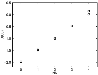
Figure 11: Plot of the isotropic hyperfine density recorded at different copper sites in clusters of various sizes for YBa₂Cu₃O₆ against the number of nearest copper neighbors at that specific site.

By a slight generalization of the ansatz (27) it is also possible to include results from clusters with lower multiplicities in the determination of on-site and hyperfine fields. We write

$$D(\textrm{Cu}_{i})=\alpha_{iso}\rho_{s}(\textrm{Cu}_{i})+\beta_{iso}\sum_{j\in NN}\rho_{s}(\textrm{Cu}_{j})$$ (28)

and similarly

$$T^{zz}(\textrm{Cu}_{i})=\alpha_{dip}^{z}\rho_{s}(\textrm{Cu}_{i})+\beta_{dip}^{z}\sum_{j\in NN}\rho_{s}(\textrm{Cu}_{j}).$$ (29)

For the hyperfine fields at the oxygen site, we make a completely analogous ansatz:

$$D(\textrm{O}_{i})=\gamma_{iso}\sum_{j\in NN}\rho_{s}(\textrm{Cu}_{j})$$ (30)

and

$$T^{zz}(\textrm{O}_{i})=\gamma_{dip}^{z}\sum_{j\in NN}\rho_{s}(\textrm{Cu}_{j}).$$ (31)

The connection between the fitting parameters $\alpha$ through $\gamma$ and the actual hyperfine parameters is then given by scaling with the expected spin density in the infinite cluster for which we find a good estimate in the center of the largest Cu₁₃ clusters with ferromagnetic spin multiplicity for each substance, i.e. $a_{iso}=\rho_{s}(\textrm{Cu})\alpha_{iso}$ etc..

The quality of the ansatz can be estimated by suitably chosen plots as e.g. a plot of $D(\textrm{Cu}_{i})/\rho_{s}(\textrm{Cu}_{i})$ against $\sum_{j\in NN}\rho_{s}(\textrm{Cu}_{j})/\rho_{s}(\textrm{Cu}_{i})$. (see Fig. 12). From the straight line, the fitting parameters $\alpha_{iso}$ and $\beta_{iso}$ are determined and scaled with the expected spin density in the infinite cluster – as noted above – to get the hyperfine parameters $a_{iso}=-1.94$ a${}_{B}^{-3}$ and $b_{iso}=0.77$ a${}_{B}^{-3}$. The corresponding values for the dipolar hyperfine coupling are $a_{dip}^{\parallel}=-3.55$ a${}_{B}^{-3}$ and $b_{dip}^{\parallel}=0.08$ a${}_{B}^{-3}$. These values are very similar to the ones obtained with the simpler ansatz which shows that the two different kinds of ansatz yield effectively the same results. Because in the second ansatz more clusters are included we quote in the following these results.

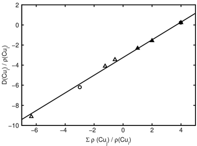
Figure 12: Plot of $D(\textrm{Cu}_{i})/\rho_{s}(\textrm{Cu}_{i})$ against $\sum_{j\in NN}\rho_{s}(\textrm{Cu}_{j})/\rho_{s}(\textrm{Cu}_{i})$ for YBa₂Cu₃O₆. Closed symbols originate from the cluster with ferromagnetic multiplicity $M=14$ and open symbols denote results for antiferromagnetic multiplicity $M=6$. Circles are for values where Cu_i is in the center of the cluster whereas points for off-center coppers are plotted with triangles.

	La2CuO4	YBa2Cu3O6	YBa2Cu3O7	YBa2Cu4O8
$a_{iso}$	$-$1.94	$-$2.09	$-$2.03	$-$2.08
$b_{iso}$	0.77	0.57	0.50	0.55
$a_{dip}^{\parallel}$	$-$3.55	$-$3.38	$-$3.40	$-$3.38
$b_{dip}^{\parallel}$	0.08	0.05	0.06	0.06
$c_{iso}$	0.64	0.63	0.62	0.60
$c_{dip}^{\parallel}$	0.40	0.40	0.39	0.42
$c_{dip}^{\perp}$	$-0.20$	$-0.21$	$-0.21$	$-0.22$
$c_{dip}^{zz}$	$-0.20$	$-0.19$	$-0.18$	$-0.20$

Table 6: Theoretical values for the hyperfine parameters at the planar copper and oxygen sites in the four substances determined with the more sophisticated ansatz II using Cu₁₃ clusters with ferromagnetic and antiferromagnetic spin arrangement. All values are given in units of a${}_{B}^{-3}$.

In Table 6 all hyperfine parameters as determined using the ansatz II can be found. We note that for the oxygen $c_{dip}^{\parallel}$ refers to the direction along the bond between the two NN coppers, $c_{dip}^{\perp}$ is perpendicular to the bond but still in the CuO₂ plane, while $c_{dip}^{zz}$ denotes the direction perpendicular to the plane.

The contribution to the hyperfine fields that originate from spin-orbit coupling $a^{\alpha}_{so}$ are expected to be small in the case of oxygen. For copper, however, they are of the same order of magnitude as $a_{iso}$ and $a_{dip}$. We are not in a position to determine them at the same level of accuracy as $a_{iso}$ and $a_{dip}$ and are thus forced to rely on a reasonable estimate. In the frame of an atomic picture with a single missing electron in the $3d_{x^{2}-y^{2}}$ orbital the dipolar and spin orbit hyperfine interactions are given by (Ref. [bib:bleaney, ])

$$a_{dip}^{\parallel}=-\frac{4}{7}\langle\>r^{-3}\>\rangle,\,a_{so}^{\parallel}=-\frac{62}{7}k\langle\>r^{-3}\>\rangle\,\textrm{and}\,a_{so}^{\perp}=-\frac{11}{7}k\langle\>r^{-3}\>\rangle.$$ (32)

(A value of $k=-0.044$ was estimated in Ref. [bib:monien1990, ]). In a molecule or solid where the missing electron spends some time on the oxygen ligands these expressions have to be modified. A simple modification is to replace the expression for $a_{dip}^{\parallel}$ by multiplying it with $2-N_{x^{2}-y^{2}}$ $a^{-3}_{B}$. Using the values $\langle\>r^{-3}\>\rangle=8.042$ (Sec. IVD) and $N_{x^{2}-y^{2}}=1.363$ (Table V) we obtain for La₂CuO₄ $a_{dip}^{\parallel}=-2.93$ which is reasonably close to the directly determined value of $-3.55$ since actually the spin density should be used instead of the charge density.

For the estimation of the spin-orbit contributions we thus assume that the relations (32) still hold in the cluster such that $a_{so}^{\parallel}$ = $15.5ka_{dip}^{\parallel}$ and $a_{so}^{\perp}=2.75ka_{dip}^{\parallel}$. The resulting values are given in Table 7.

In Table 8 we collect the calculated values for the total hyperfine parameters expressed in terms of densities and also in terms of interaction energies which we denote by capital letters. The latter are defined by ${}^{63}A_{tot}^{\alpha}=\hbar\gamma_{e}\hbar^{63}\gamma a_{tot}^{\alpha}$ and similarly for the ${}^{63}B$ and ${}^{17}C$ and (as the notation) indicates depend on the particular isotope.

	La2CuO4	YBa2Cu3O6	YBa2Cu3O7	YBa2Cu4O8
$a_{so}^{\parallel}$	2.43	2.32	2.27	2.28
$a_{so}^{\perp}$	0.43	0.41	0.40	0.40

Table 7: Estimation for spin-orbit contributions to the hyperfine fields at the copper site in the various substances. All values are given in atomic units.

	La2CuO4	YBa2Cu3O6	YBa2Cu3O7	YBa2Cu4O8
$a_{tot}^{\parallel}$	$-3.06$	$-3.15$	$-3.16$	$-3.18$
$a_{tot}^{\perp}$	0.26	0.01	0.07	0.01
$b_{tot}^{\parallel}$	0.85	0.62	0.56	0.61
$b_{tot}^{\perp}$	0.73	0.52	0.47	0.52
$c_{tot}^{\parallel}$	1.04	1.03	1.01	1.02
$c_{tot}^{\perp}$	0.44	0.42	0.41	0.38
$c_{tot}^{c}$	0.44	0.44	0.44	0.40
${}^{63}A_{tot}^{\parallel}$	$-1.79$	$-1.84$	$-1.85$	$-1.86$
${}^{63}A_{tot}^{\perp}$	0.15	0.01	0.04	0.01
${}^{63}B_{tot}^{\parallel}$	0.50	0.36	0.33	0.36
${}^{63}B_{tot}^{\perp}$	0.43	0.30	0.27	0.30
${}^{17}C_{tot}^{\parallel}$	0.31	0.31	0.30	0.30
${}^{17}C_{tot}^{\perp}$	0.13	0.13	0.12	0.11
${}^{17}C_{tot}^{c}$	0.13	0.13	0.13	0.12

Table 8: Contributions to the hyperfine fields at the copper site ($a$ and $b$) and at the oxygen site ($c$) in the various compounds in a${}_{B}^{-3}$ ($a,b$ and $c$) and in $\mu$eV (${}^{63}A$, ${}^{63}B$ and ${}^{17}C$). ${}^{63}A/a$ and ${}^{63}B/b$ = 0.5844 $\mu$eVa${}_{B}^{3}$ and ${}^{17}C/c$ = 0.2988 $\mu$eVa${}_{B}^{3}$.

V.2 Comparison with experiments

Although experiments cannot determine on-site and transferred hyperfine fields separately it is possible to extract various combinations of on-site and transferred fields using different experimental set-ups.

One constraint is the relation $a_{tot}^{\parallel}+4b_{tot}^{\parallel}=0$ which explains that the NMR spin shift measured with the field in $c$-direction does not change below the superconduction transition temperature $T_{c}$ in contrast to the spin shift measured with the field perpendicular to the $c$-axis. We postpone a comparison with our theoretical values to Sec. VI.3.

A second experimental determination of a combination of on-site and transferred hyperfine fields is made possible through measurements of the NMR resonance frequency, ${}^{63}\nu_{L}$, of the copper nuclei in the pure parent compounds La₂CuO₄ and YBa₂Cu₄O₆ which are in the antiferromagnetic state. This determines the local magnetic field ${}^{63}\gamma H_{loc}=2\pi^{63}\nu_{L}$ which is commonly expressed as the corresponding hyperfine field in units of an effective electronic magnetic moment $\mu_{B}^{\textit{\footnotesize{eff}}}\simeq 0.66\mu_{B}$ as $H_{loc}=|a_{tot}^{\perp}-4b_{tot}^{\perp}|\mu_{B}^{\textit{\footnotesize{eff}}}$.

For La₂CuO₄ the theoretical value for $\Delta\equiv|a_{tot}^{\perp}-4b_{tot}^{\perp}|$ is 2.66 whereas the measuredbib:tsuda1988 frequency of 93.85 MHz corresponds to $\Delta=2.01$. For YBa₂Cu₃O₆ we get $\Delta=1.90$ in good agreement with the experimentbib:yasuoka1988 (89.89 MHz) which leads to $\Delta=1.92$.

Sometimes the measured anisotropy between the copper spin-lattice relaxation times ${}^{63}T_{1,\parallel}/^{63}T_{1,\perp}$ has also been used to extract information about the hyperfine coupling constants. This, however, is only possible for the two extreme conditions of totally antiferromagnetic correlations (which is never achieved for the doped samples) or of no correlations, which would require measurements at very high temperatures.

	$a)$	$b)$	$c)$	$d)$	$e)$
${}^{63}A_{tot}^{\parallel}$	$-1.85$	$-1.86$	$-1.76$	$-1.61$	$-0.94$
${}^{63}A_{tot}^{\perp}$	0.04	0.23	$-0.10$	0.29	0.17
${}^{63}B_{iso}$	0.29	0.34	0.41	0.40	0.23

Table 9: Contributions to the hyperfine fields at the copper site in YBa₂Cu₃O₇. $a)$ this work, $b)$ Ref. [bib:monien1990, ], $c)$ Ref. [bib:walstedt1990a, ], $d)$ Ref. [bib:zha, ], and $e)$ Ref. [bib:nandor, ].

In Table 9 we compare our values for the hyperfine interaction energies with those published by several authors. An inspection shows that the deviations are not large but sufficiently strong to render further interpretations questionable. In particular, until more reliable values for the influence of the spin-orbit coupling on the hyperfine fields are known, it is prohibitive to make more precise statements.

VI Chemical shieldings and Paramagnetic Field Modifications

VI.1 General remarks

Very early after the discovery of the high temperature superconductors, numerous measurements of Knight shifts at various nuclei have been performed. For optimally doped YBa₂Cu₃O₇, the Knight shift ${}^{63}\!K^{\perp}$ of the planar copper for the field applied perpendicular to the $c$-axis is temperature independent above $T_{c}$ and drops below $T_{c}$ with decreasing temperature to ${}^{63}\!K^{\perp}(T=0)$. The behavior above $T_{c}$ is to be expected for a temperature independent Pauli spin susceptibility. The reduction of the Knight shift below $T_{c}$ was explained by the formation of Cooper pairs which are – due to their vanishing total spin – not available for polarization by a magnetic field and therefore do not contribute to the Knight shift. At zero temperatures, all charge carriers were assumed to be bound in Cooper pairs and the remaining Knight shift ${}^{63}\!K^{\perp}(T=0)$ was attributed to the temperature and doping independent chemical shift. The temperature dependence of ${}^{63}\!K^{\perp}(T)$ in the superconducting state depends on the symmetry of the pairing state and most NMR experiments were better explained by $d$-wave pairing. (For underdoped materials, the decline of the Knight shift ${}^{63}\!K^{\perp}(T)$ with lowering temperatures sets in already at temperatures above $T_{c}$ which has attributed to the opening of a spin pseudogap.)

The copper Knight shift ${}^{63}\!K^{\parallel}(T)$ with the applied field along the crystallographic $c$ axis, however, is constant over the whole temperature range, i.e. it is completely unaffected by the superconducting transition. Therefore, it was concluded that all of the measured Knight shifts are of chemical origin. The vanishing spin part of the Knight shifts was then explained by an accidental cancellation of the on-site and transferred hyperfine fields. As already mentioned in Sec. V our calculations of on-site and transferred hyperfine fields in substances of the La and Y families do not support this cancellation. In this section we will, in addition, give further evidence that the above sketched explanation of the Knight shifts in cuprates needs careful revision based on first-principles calculations of chemical shifts at the planar copper nuclei in La₂CuO₄, YBa₂Cu₃O₆, and YBa₂Cu₃O₇. Before we report on the results of these calculations, we point out that copper Knight shift measurements have long been misinterpreted due to a wrong assumption on the magnetic properties of the reference substance. As a remedy we introduce a new term, the paramagnetic field modification.

VI.2 The role of the reference substance

Knight shift measurements are in fact measurements of differences in resonance frequencies of a nuclear species $k$, in a target substance ($t$) and in a reference substance ($r$).

$${}^{k}\!K(t-r)=\frac{{}^{k}\nu(t)-\mbox{${}^{k}\nu$}(r)}{\mbox{${}^{k}\nu$}(r)}.$$ (33)

For copper Knight shift measurements the most often used reference substance is the monovalent CuCl. The Knight shifts are made up of two parts, a temperature independent chemical shift, ${}^{k}\!K_{L}$, and a spin shift, ${}^{k}\!K_{s}$. In this section we consider the contribution of the chemical shift.

For a theoretical determination of chemical shifts we need to know the chemical shieldings, $\sigma$, in the target and the reference substance. The connection to the measured chemical shift, ${}^{k}\!K_{L}^{ii}(t-r)$, is given by

$${}^{k}\!K_{L}^{ii}(t-r)=\frac{{{}^{k}\sigma^{ii}(r)}-{{}^{k}\sigma^{ii}(t)}}{1+{{}^{k}\sigma^{ii}(r)}}\simeq{{}^{k}\sigma^{ii}(r)}-{{}^{k}\sigma^{ii}(t)},$$ (34)

or, with the separation of ${}^{k}\sigma^{ii}$ into diamagnetic $(d)$ and paramagnetic $(p)$ parts of the shieldings, by

$${}^{k}\!K_{L}^{ii}(t-r)={{}^{k}\sigma_{d}^{ii}(r)}+{{}^{k}\sigma_{p}^{ii}(r)}-{{}^{k}\sigma_{d}^{ii}(t)}-{{}^{k}\sigma_{p}^{ii}(t)}.$$ (35)

As we have shown in Ref. [bib:renold2003, ] the differences between ${}^{63}\sigma_{d}^{ii}(r)$ and ${}^{63}\sigma_{d}^{ii}(t)$ are negligible and we can therefore write

$${}^{63}\!K_{L}^{ii}(t-r)={{}^{63}\sigma_{p}^{ii}(r)}-{{}^{63}\sigma_{p}^{ii}(t)}.$$ (36)

It has long been assumed, that the paramagnetic contribution of the shielding in the target substance, CuCl, is small. We have shown, however, ($i$) by a direct quantum chemical calculation and ($ii$) by referring to measurements of the chemical shieldings using atomic beam techniques, that ${}^{63}\sigma_{p}^{ii}($CuCl$)=1500$ ppm. In view of typical chemical shieldings at copper nuclei in cuprates (see Sec. VI.3) this contribution is sizeable and cannot be neglected.

The quantities of interest in Eq. (36) are, of course, not the chemical shifts, ${}^{63}\!K_{L}^{ii}(t-r)$, but rather the contributions of the target, i.e. $-^{63}\sigma_{p}^{ii}(t)$. To avoid misinterpretations we find it most convenient to introduce here a new quantity, the paramagnetic field modification:

$${}^{63}\overline{K}_{L}^{ii}(t)\equiv-^{63}\sigma_{p}^{ii}(t)={{}^{63}\!K_{L}^{ii}(t-r)}-{{}^{63}\sigma_{p}^{ii}(r)}.$$ (37)

It is important to note that this paramagnetic field modification ${}^{63}\overline{K}_{L}^{ii}(t)$ is independent of the reference substance.

VI.3 Theoretical determination of chemical shifts and comparison to experiment

For a detailed description about the determination of chemical shifts in the framework of the cluster technique, we refer the reader to Refs. [bib:renold2003, ; bib:renolddiss, ]. Here we just mention the important steps.

Calculations have been performed for La₂CuO₄, YBa₂Cu₄O₆, and YBa₂Cu₃O₇ using clusters with five copper atoms in the plane. Larger clusters have not been employed systematically since the determination of the shielding constants with the large basis sets that are required for accurate calculations are extremely time consuming. Test calculations in Cu₉ clusters for La₂CuO₄ have shown, however, that the results do not change upon enlarging the clusters.

In Fig. 13 theoretical results for ${}^{63}\overline{K}_{L}^{\parallel}$ (${}^{63}\overline{K}_{L}^{\perp}$) are displayed with solid bars in the left (right) panel. The dotted bars denote results reported from various experiments. It is observed that for the applied field in the plane (right panel of Fig. 13) the theoretical values are in general slightly lower than the values obtained from experiments. For fields parallel to the $c$ axis, theory predicts values for ${}^{63}\overline{K}_{L}^{\parallel}$ (left panel) that are only about half as large as the experimental results. We find, however, that the paramagnetic field modifications at the planar copper sites hardly depend on the specific cuprate.

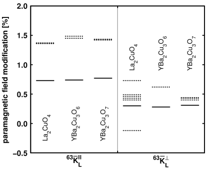
Figure 13: Paramagnetic field modifications at the planar copper site in the considered substances both for fields along the $c$ axis, ${}^{63}\overline{K}_{L}^{\parallel}$, (left panel) and for fields in the plane, ${}^{63}\overline{K}_{L}^{\perp}$ (right panel). Results obtained theoretically (experimentally) are displayed with solid (dashed) bars. The experimental data are taken from Ref. [bib:ohsugi, ] (La_2-xSr_xCuO₄), from Refs. [bib:mali1991, ; bib:pozzi1999, ] (YBa₂CuO₆) and from Refs. [bib:barrett1991, ; bib:walstedt1990, ; bib:takigawa1991, ] (YBa₂CuO_7-δ).

We have, at present, no explanation for the discrepancy between theory and experiment. We would like to point out, however, that it was shown in Refs. [bib:zheng99_1248, ; bib:zheng00_tlperp, ] that the measured Knight shifts below $T_{c}$ are field dependent and drop when reducing the applied magnetic field $H$. The theoretical calculations, of course, are in the limit of $H\rightarrow 0$. Furthermore, it is also possible that impurities induce a finite density of states at $T=0$, as was proposed in Ref. [bib:ohsugi, ]. Both of the above two ideas imply that the measured Knight shifts at $T=0$ are not entirely of chemical origin but also have contributions from spin degrees of freedom.

The temperature independence of the copper Knight shift when measured with the field in c-direction is most easily explained by an incidentend cancellation of the on-site and transferred hyperfine fields, i.e. $a_{tot}^{\parallel}+4b_{tot}^{\parallel}\approx 0$. In Table X we present the values calculated for $1+a_{tot}^{\parallel}/4b_{tot}^{\parallel}$ for the four substances under consideration. The values are close to zero but differ among the various compounds. For La₂CuO₄, a small positive value of 0.1 is obtained. for YBa₂Cu₃O₇, however, we obtain $-0.4$. This difference is from the theoretical point of view easily explained by the fact that the transferred hyperfine field $b_{tot}^{\parallel}$ in YBa₂Cu₃O₇ is smaller than in La₂CuO₄ due to the buckling of the planar oxygen atoms. It is evident that the calculations for one compound may fail to give the cancellations necessary for the easy explanation of the temperature independence of ${}^{63}K^{\parallel}$. To explain the behavior of ${}^{63}K^{\parallel}$ both in La₂CuO₄ and in the Y-compounds already requires a double coincidence. In addition, measurements on the electron doped material PrLaCeCuO₄ by Zheng et al. bib:Zheng also exhibit a temperature independent ${}^{63}K^{\parallel}$. In view of the differences in the lattice parameters in all three substances it is extremely intriguing that these cancellations of on-site and transferred hyperfine fields which are basically determined by chemistry, occur.

	1 + $a_{tot}^{\parallel}/4b_{tot}^{\parallel}$
La2CuO4	$\,\,\,\,0.105$
YBa2Cu3O6	$-$0.278
YBa2Cu3O7	$-$0.402
YBa2Cu4O8	$-$0.292

Table 10: Theoretical relations for the total hyperfine fields at the central copper atom.

VII Summary and Conclusions

We have performed large-scale ab-initio cluster computations of cuprates in order to determine the local electronic structure. The convergence of these local properties with respect to the cluster size is very good. An analysis of the charge and spin distribution in terms of contributions from the various MO and AO reveals distinguished features in all compounds under consideration. First, the copper 3$d_{x^{2}-y^{2}}$ AO is occupied by about 1.4 and the 3$d_{3z^{2}-r^{2}}$ AO by about 1.9 electrons. The oxygen 2$p_{\sigma}$ AO contains roughly 1.65 electrons. This implies a total of 1.4 intrinsic holes per unit which is compensated by $0.4-0.5$ electrons in the copper 4$s$ AO. These partial occupancies of the non-spherical AO mainly determine the EFG values. The 4$s$ AO is involved in the transferred hyperfine field. Good agreement between the calculated and measured copper EFG is found. The EFG values essentially depend on the differences between the Mulliken populations of the 3$d_{3z^{2}-r^{2}}$ and the 3$d_{x^{2}-y^{2}}$ AO.

Simulating doping by two different methods shows that all these occupancies smoothly change and the general trends of changing copper EFG with doping level are reproduced. The removal of one electron by a dopant atom in the intra-layer induces only half a hole in the CuO₂ plane. The other half is in out-of-plane orbitals.

Spin-polarized calculations with various spin multiplicities enabled the determination of the antiferromagnetic exchange coupling and the various hyperfine fields. The contribution of the spin-orbit coupling, however, has only been approximately determined. The calculated total hyperfine fields are in rough agreement with those deduced from experiments. The values for the sum $a_{tot}^{\parallel}+4b_{tot}^{\parallel}$ are small but differ considerably among the substances under consideration. This in sharp contrast to the requirements set by the temperature independence of the copper Knight-shift ${}^{63}K^{\parallel}$ observed in very different cuprates.

We conclude that the out-of-plane orbital 3$d_{3z^{2}-r^{2}}$ and the 4$s$ orbital play a more important role than commonly assumed.

- (1) J.G. Bednorz and K. A. Müller, Z. Phys. 64, 189 (1986).
- (2) W.E. Pickett, Rev. Mod. Physics 61, 433 (1989).
- (3) P. Hüsser, H.U. Suter, E.P. Stoll, and P.F. Meier, Phys. Rev. B 61, 1567 (2000).
- (4) S. Renold, S. Pliberšek, E.P. Stoll, T.A. Claxton, and P.F. Meier, Eur. Phys. J. B 23, 3 (2001).
- (5) A.D. Becke, Phys. Rev. A 38, 3098 (1988).
- (6) A.D. Becke, J. Chem. Phys. 88, 2547 (1988).
- (7) C. Lee, W. Yang, and R.G. Parr, Phys. Rev. B 37, 785 (1988).
- (8) M.J. Frisch, et al., Gaussian 03, Revision C.02, Gaussian, Inc., Wallingford CT, 2004.
- (9) H.U. Suter, E.P. Stoll, P. Hüsser, S. Schafroth, and P.F. Meier, Physica C 282-287, 1639 (1997).
- (10) P.G. Radaelli, D.G. Hinks, A.W. Mitchell, B.A. Hunter, J.L. Wagner, B. Dabrowski, K.G. Vandervoort, H.K. Viswanathan, and J.D. Jorgenson, Phys. Rev. B 49, 4163 (1994).
- (11) R.J. Cava, A.W. Hewat, E.A. Hewat, B. Batlogg, M. Marezio, K.M. Rabe, J.J. Krajewski, W.F. Peck, Jr. and L.W. Rupp, Jr., Physica C 165, 419 (1990).
- (12) P. Bordet, C. Chaillout, J.J. Capponi, J. Chenavas, M. Marezio, Nature 327, 687 (1987).
- (13) P. Fischer, J. Karpinski, E. Kaldis, E. Jilek, and S. Rusiecki, Solid State Commun. 70, 531 (1989).
- (14) B. Keimer, N. Belk, R.J. Birgeneau, A. Cassanho, C.Y. Chen, M. Greven, M.A. Kastner, A. Aharony, Y. Endoh, R.W. Erwin, and G. Shirane, Phys. Rev. B 46, 14034 (1992).
- (15) S. Shamoto, M. Sato, J.M. Tranquada, B.J. Sternlieb, and G. Shirane. Phys. Rev. B 48, 13817 (1993).
- (16) D. Muñoz, I. de P.R. Moreira, and F. Illas, Phys. Rev. B 65, 224521 (2002).
- (17) in the present context it is not necessary to distinguish between the different spin projections.
- (18) E.P. Stoll, P.F. Meier, and T.A. Claxton, Phys. Rev. B 65, 64532-1 (2002).
- (19) E.P. Stoll, P.F. Meier, and T.A. Claxton, Int. J. of Mod. Phys. B, 17, 3329 (2003).
- (20) C. Bersier, S. Renold, E.P. Stoll, and P.F. Meier, J. Phys.: Condens. Matter, 18, 7481 (2006).
- (21) C. Bersier, E.P. Stoll, P.F. Meier, and T.A. Claxton, Journal of Superconductivity: Incorporating Novel Magnetism, 15, 403 (2002).
- (22) E.P. Stoll, P.F. Meier, and T.A. Claxton, J. Phys.: Condens. Matter, 15, 7881 (2003).
- (23) Shigeki Ohsugi, Yoshio Kitaoka, Kenji Ishida, Guo-qing Zheng, and Kunisuke Asayama, J. Phys. Soc. Japan, 63, 700 (1994).
- (24) T. Imai, C.P. Slichter, K. Yoshimura, and K. Kosuge, Phys. Rev. Lett. 70, 1002 (1993).
- (25) J. Haase, O.P. Sushkov, P. Horsch, and G.V.M. Williams, Phys. Rev. B 69, 094504 (2004).
- (26) C. Ambrosch-Draxl, P. Süle, H. Auer, and E.Ya. Sherman, Phys. Rev. B 67, 100505 (2003).
- (27) S. Renold and P.F. Meier, Journal of Superconductivity: Incorporating Novel Magnetism, 16, 483 (2003).
- (28) E.S. Bošin and S.J.L. Billinge, Phys. Rev. B 72, 174427 (2005).
- (29) C.P. Slichter, in Strongly Correlated Electronic Materials, The Los Alamos Symposium, edited by K.S. Bedell, Z. Wang, D. Meltzer, A.V. Balatsky, and E. Abrahams (Addison-Wesley, Reading, MA, 1993), p. 427.
- (30) P. Pyykkö, Mol. Phys, 99, 1617 (2001).
- (31) M. Matsumura, M. Mali, J. Roos, and D. Brinkmann, Phys. Rev. B 56, 8938 (1997).
- (32) D. Brinkmann, in Materials and Cristallographic Aspects of HTc-Superconductivity, edited by E. Kaldis (Kluwer, 1994), p. 225.
- (33) P. Hüsser, E. Stoll, H.U. Suter, and P.F. Meier, Physica C 294, 217 (1998).
- (34) A. Kanigel and A. Keren, Phys. Rev. B 74, 012505 (2006).
- (35) B. Bleaney, K.D. Bowers, and M.H.L. Pryce, Proc. R. Soc. London, Ser. A 228, 166 (1955).
- (36) H. Monien, D. Pines, and C.P. Slichter, Phys. Rev. B41, 11120 (1990).
- (37) T. Tsuda, T. Shimizu, H. Yasuoka, K. Kishio, and K. Kitazawa, J. Phys. Soc. Japan 57, 2908 (1988).
- (38) H. Yasuoka, T. Shimizu, Y. Ueda, and K. Kosuge, J. Phys. Soc. Japan 57, 2659 (1988).
- (39) R.E. Walstedt and W.W. Warren, Science 248, 1082 (1990).
- (40) Y. Zha, V. Barzykin, D. Pines, Phys. Rev. B54, 7561 (1996).
- (41) V.A. Nandor, J.A. Martindale, R.W. Groves, O.M. Vyaselev, C.H. Pennington, L. Hults and J.L. Smith, Phys. Rev. B60, 6907 (1999).
- (42) S. Renold, T. Heine, J. Weber, and P.F. Meier, Phys. Rev. B67, 024501 (2003).
- (43) S. Renold, First-principles studies of electonic and magnetic properties in cuprates, thesis, Zürich (2004).
- (44) S. Ohsugi, Y. Kitaoka, K. Ishida, G.-q. Zheng, and K. Asayama, J. Phys. Soc. Japan 63, 700 (1994).
- (45) M. Mali, I. Mangelschots, H. Zimmermann, and D. Brinkmann, Physica C 175, 581 (1991).
- (46) R. Pozzi, M. Mali, D. Brinkmann, and A. Erb, Phys. Rev. B60, 9650 (1999).
- (47) S.E. Barrett, J.A. Martindale, D.J. Durand, C.H. Pennington, C.P. Slichter, T.A. Friedmann, J.P. Rice, and D.M. Ginsberg, Phys. Rev. Lett. 66, 108 (1991).
- (48) R.E. Walstedt, W.W. Warren, Jr., R.F. Bell, R.J. Cava, G.P. Espinosa, L.F. Schneemeyer, and J.V. Waszczak, Phys. Rev. B41, 9574 (1990).
- (49) M. Takigawa, A.P. Reyes, P.C. Hammel, J.D. Thompson, R.H. Heffner, Z. Fisk, and K.C. Ott, Phys. Rev. B43, 247 (1991).
- (50) G.-q. Zheng, W.G. Clark, Y. Kitaoka, K. Asayama, Y. Kodama, P. Kuhns, and W. G. Moulton, Phys. Rev. B60, R9947 (1999).
- (51) G.-q. Zheng, H. Ozaki, W. G. Clark, M. Sakai, Y. Kitaoka, Y. Kodama, T. Kondo, Y. Shimakawa, Y. Kubo, P. Kuhns, A.P. Reyes, and W.G. Moulton, Physica C 341-348, 819 (2000).
- (52) Guo-qing Zheng, T. Sato, Y. Kitaoka, M. Fujita, and K. Yamada, Phys. Rev. Lett. 90, 197005 (2003).