Insulator-metal transition on the triangular lattice
Abstract
Mott insulators with a half-filled band of electrons on the triangular lattice have been recently studied in a variety of organic compounds. All of these compounds undergo transitions to metallic/superconducting states under moderate hydrostatic pressure. We describe the Mott insulator using its hypothetical proximity to a spin liquid of bosonic spinons. This spin liquid has quantum phase transitions to descendant confining states with Néel or valence bond solid order, and the insulator can be on either side of one of these transitions. We present a theory of fermionic charged excitations in these states, and describe the route to metallic states with Fermi surfaces. We argue that an excitonic condensate can form near this insulator-metal transition, due to the formation of charge neutral pairs of charge and charge fermions. This condensate breaks the lattice space group symmetry, and we propose its onset as an explanation of a low temperature anomaly in -(ET)2Cu2(CN)3. We also describe the separate BCS instability of the metallic states to the pairing of like-charge fermions and the onset of superconductivity.
I Introduction
The organic superconductors have proved to be valuable systems for exploring strong correlation physics near the metal-insulator transition: it is possible to tune parameters across the metal-insulator transition by moderate pressure, while maintaining a commensurate density of carriers. Of particular interest are the series of compounds which realize a half-filled band of electrons on a triangular lattice. In the insulator, three distinct ground states are realized in closely related compounds: (i) a Néel ordered state kanoda1 in -(ET)2 Cu[N(CN)2]Cl (ii) a recently discovered valence bond solid (VBS) state kato1 ; kato2 ; kato3 in EtMe3P[Pd(dmit)2]2, and (iii) an enigmatic spin liquid state kanoda0 ; kanoda2 ; palee in -(ET)2Cu2(CN)3. Under pressure, all these compounds undergo a transition to a superconducting state.
The nearest-neighbor Heisenberg antiferromagnet on the triangular lattice is believed to have a small, but non-zero, average magnetic moment singh ; misguich ; motrunich ; senechal . However, perturbations such as ring and second-neighbor exchange are likely to be present near the metal-insulator transition, and these presumably yield the non-magnetic states noted above. This paper will examine the organic compounds from the perspective of a particular spin-liquid insulating ground state: the spin liquid of bosonic spinons proposed in Refs. sstri, ; ashvin, . An advantage of this state is that it is a very natural starting point for building the entire phase diagram: theories of the transitions out of this spin liquid state into the magnetically ordered (Néel) state css and the valence bond solid state ms have already been presented, thus realizing the three classes of insulators which are observed in these compounds.
The core analysis of this paper concerns the insulator-to-metal transition on the triangular lattice senechal out of the spin liquid state. The spin-charge separation of the insulating spin liquid state (and the associated topological order) will survive across the transition into the metallic state, and so this is a insulator-metal transition between two ‘exotic’ states. However, our theory generalizes easily to the other ‘non-exotic’ insulators with conventional order noted above: in these cases it is the conventional order which survives across the transition, rather than the topological order. Thus our study of the spin liquid state offers a convenient context in which to study the insulator-metal transition, with a focus on the charged excitations in the simplest situation. Subsequently, we can include the spin-sector instabilities of the spin liquid to conventionally ordered confining states; these do not modify the physics of the insulator-metal transition in a significant manner.
Our perspective on the insulator-metal transition should be contrasted to that in dynamical mean-field theory dmft ; ross (DMFT). DMFT begins with a correlated metallic state, and presents a theory of the metal-to-insulator transition. Partly as a consequence of its focus on the metal, it does a rather poor job of capturing the superexchange interactions in the insulator, and the consequent resonating valence bond (RVB) correlations. Instead, we begin with a theory of RVB-like correlations in the insulator, and then develop a theory of the charged excitations; the closing of the gap to these charged excitations describes the insulator-to-metal transition. A theory of the closing of the charge gap in an RVB insulator has also been discussed recently by Hermele hermele , but for an insulator with gapless fermionic spinons on the honeycomb lattice.
For a half-filled band, our main result is that prior to reaching the metallic state, the insulator has an instability to a state with exciton condensationrice , associated with the pairing of fermions of charge with fermions of charge . As in the conventional theory rice , the pairing arises because of the attractive Coulomb interaction between these oppositely charged fermions, while the charge gap to these fermionic excitations is still finite, but small. The excitonic insulator maintains the charge gap, but is associated with a breaking of the lattice space group symmetry which we shall describe. Eventually, Fermi surfaces of charge fermions appear, leading to a metallic state in which the excitonic instability (and the lattice symmetry breaking) can also survive.
We propose that the above instability offers a resolution of a central puzzle in the properties of the ‘spin liquid’ compound -(ET)2Cu2(CN)3. At a temperature around 10K a feature is observed kanoda2 ; kanoda3 in nearly all observables suggesting a phase transition into a mysterious low temperature correlated state. An important characteristic of this compound is the indication from optical conductivity measurements kanoda4 that the charge gap of this insulator is quite small, suggesting its proximity to the metal-insulator transition even at ambient pressure. We propose the 10K transition occurs in the charge sector, and is a consequence of the appearance of the excitonic insulator. Observation of the lattice symmetry breaking associated with the excitonic insulator state is an obvious experimental test of our proposal. There is a suppression of the spin susceptibility below the transition, and this can arise in our theory from the strong coupling between the fermionic charge carriers and the spinons; this coupling is given by the large hopping term, in a - model, and we will discuss a number of consequences of this term.
The spin liquid state upon which our excitonic insulator state is based has a gap to all spin excitations, and this is potentially an issue in applications to -(ET)2Cu2(CN)3. However, as we have already mentioned above, our theory is easily extend across the critical point to the onset of magnetic order. We propose that the spin gap is very small due to proximity to this critical point, and that along with the effect of impurities, this can possibly explain the large density of states of gapless spin excitations observed in Ref. kanoda2, . Indeed, the dependence of the spin susceptibility fits the predictions of the nearest-neighbor Heisenberg antiferromagnet reasonably well, and the latter model is believed to be very close to a quantum phase transition at which the Néel order disappears singh .
The central focus of this paper will be on the charged excitations of the spin liquid.
These will spinless fermions of charge : we call the charge
fermion a ‘holon’, and the charge fermion a ‘doublon’. We will begin with a theory of the dispersion
spectrum of single holons and doublons in Section II. The remaining sections of the paper will consider
various many-body states that can appears in a finite density liquid of these fermions. The states we will find are:
(i) Excitonic condensates: This will be discussed in Section III.
Here there is an instability towards the pairing between a holon and doublon to form a condensate
of neutral bosons. The only physical symmetry broken by this pairing is the space group symmetry
of the triangular lattice, and so the state with an excitonic condensate has a spatial modulation
in the electronic charge density. We find this state as an instability of the insulating spin liquid,
which then reaches an insulating state with an excitonic condensate. However, eventually Fermi surfaces
of holons and doublons can develop, leading to a metallic state with an excitonic condensate.
(ii) Metals: As the repulsion energy in a Hubbard model becomes smaller,
we will find that Fermi surfaces of the holons and doublons can appear (as has just been noted
in the discussion of excitonic condensates). Such states are realizations of ‘algebraic charge liquids’ (ACLs)
introduced recently in Ref. acl, , and these will be discussed further
in Section IV. The simplest such states inherit the topological order of the spin liquid.
The areas enclosed by the Fermi surfaces in these fractionalized metallic states obey a modified Luttinger
theorem, whose form will be discussed in Section IV. We will also discuss the possible
binding of holons and doublons to spinons, and the eventual appearance of conventional Fermi liquid
metallic states.
(iii) Superconductors: The metallic states above are also susceptible to
a conventional BCS instability to a superconducting state, by the condensation of bosons
of charge . This will be discussed in Section V. The required
attractive interactions between pairs of holons (or pairs of doublons) is driven by the exchange of
spinon excitations of the spin liquid. We will compute this interaction, and show that it favors
a superconductor in which the physical electronic pair operators have a pairing signature.
II Charged excitations of the spin liquid
As we noted in Section I, the central actor in our analysis, from which all phases will be derived, is the insulating spin liquid state on the triangular lattice sstri ; ashvin . A review of its basic properties, using the perspective of the projective symmetry group wenpsg is presented in Appendix A.
Here we will extend the antiferromagnet to the - model on the triangular lattice and describe the spectrum of the charged holon and doublon excitations of the spin liquid. Because of the spin-charge separation in the parent spin liquid, both the holons and doublons are spinless, but carry a unit charge of the gauge field of the spin liquid. The distinct metallic, insulating, and superconducting phases which can appear in a system with a finite density of holons and doublons are described in the subsequent sections.
We consider the usual - model on a triangular lattice:
| (1) |
where are sites of the triangular lattice. As discussed in Appendix A, the spin liquid is realized by expressing the the spins in terms of Schwinger bosons . Here, we introduce spinless, charge , fermionic holons, , and spinless, charge , fermionic doublons, . The , , and all carry a unit charge. At half-filling, the density of holons must equal the density of doublons, but our formalism also allows consideration of the general case away from half-filling with unequal densities. We can now expression the electron annihilation operator in terms of the these degress of freedom by
| (2) |
where is the antisymmetric unit tensor. A similar spin-charge decomposition of the electron into spinons was discussed in the early study of Zou and Anderson Zou1988 , but with the opposite assignment of statistics i.e. fermionic spinons and bosonic holons. In our case, the choice of statistics is dictated by the choice of the spin liquid we are considering.
With the spin liquid background, the charge degrees of freedom acquire a kinetic energy from the hopping term. To see this, plug the separation (2) into the -term in equation (1)
| (3) |
Replacing the spinon operators with the mean field expectation values of the spinon pair operators discussed in Appendix A, we obtain
where and are the expectation values defined in Eq. (77). Using Fourier transform to convert this to momentum space, we obtain
| (4) |
where is defined as
| (5) |
Here we are using the oblique co-ordinate system shown in Fig. 1. For momentum space, we use the dual base with respect to the coordinate system. Therefore . Momenta , and are equivalent. For convenience, a third component of momentum is defined as to make formulas more symmetric.

In the complete Hamiltonian, we need a chemical potential to couple to the total charge density: when this is within the Mott gap, the density of holons and doublons will be equal and the system will be half-filled. Also, the double occupancy energy needs to be included since the number of double occupied sites is not conserved. Combining these two terms with the kinetic energy (4), we obtain
| (6) |
The above Hamiltonian can be diagonalized by Bogoliubov transformation. To do so, first write the Hamiltonian in the following matrix form:
| (7) |
where
| (8) |
and the kinetic energy matrix
| (9) |
The spectrum of quasi-particles is the eigenvalue of the matrix (9)
| (10) |
We can redefine the chemical potential to absorb the term in Eq. (10). Also, to make it simpler, define
| (11) |
Then the dispersion of the two bands looks like
| (12) |
To study the maximum and minimum position of the about dispersion, we need to first identify the stationary points of the dispersion in the Brillouin zone. This can be done by noticing that the two dependent function and in equation (12) reach stationary points simultaneously at the points listed in the first column of Table 1.
| Steady points | |||
|---|---|---|---|
| 3 | 0 | ||
| , , | -1 | 0 |
The maximal and minimal points of the bands must come from the candidates listed in Table 1. To determine which one is the maximum or minimum, we compare the energy at those stationary points, which is listed in Table 1 along with real and imaginary parts of . It is easy to see that the position of minimum and maximum depends on the sign of and the value of , and . Let us discuss two extreme case and for both and .
-
•
First, consider the extreme case . In this case the effect of the term can be ignored comparing to the term in the square root and the shape of dispersion is solely determined by the term, which is listed in the second column of table 1. Therefore the maximums locate at , and the minimal point is , for both the upper and lower bands.
Then consider the other extreme: . In this case the energy at the stationary points are
(13) (14) (15) Without the term, (13) was the maximum. However, when the term is deducted from it, it becomes smaller and can be smaller than (15). Then the maximal points of the lower band become , and . The requirement for (15) to be smaller than (13) is
(16) By minimizing the Hamiltonian the mean field parameters and we get show that the inequality (16) holds. Therefore the minimal points are , and .
-
•
For this case, notice that the dispersions of the bands for parameters and are related
(17) Therefore for the bands are up-side down. Hence the bottom of upper band and the top of the lower band are switched (see Table 2).
| Min of | Max of | ||
|---|---|---|---|
According to Eq. (17), the dispersion of the bands are flipped when changes the sign. However, since we are at zero doping, the flip of the bands only switches the name of holons and doublons, but the physics is very similar in the two cases. From minimizing the spinon mean field Hamiltonian we found that . Therefore in the following discussion we will assume that and . Consequently the maximum of valence band and the minimum of electron band comes from the row of Table 2: when the band gap is small , lower band excitations are around , and higher band excitations are around , and . It is worth noticing that the mixing term in Eq. (6), which is proportional to , vanishes at these points (see Table 1). Therefore, the Bogoliubov transformation is trivial at the center of the Fermi sea of the two types of excitations. If we assume that the Fermi sea of excitations are small, then the excitations can be identified as holons and doublons. According to the definition of quasiparticle (8), it carries the same electric charge as the original electron. Therefore the quasiparticle excitation in the upper band is doublon, and the quasihole excitation in the lower band is holon. Therefore low energy effective fields of holon () and doublon () can be defined as
| (18) | ||||
| (19) |
where denotes three minimums in doublon dispersion:
| (20) |
The positions of these excitations in the Brillouin zone are indicated in Fig. 2.
II.1 Two-band model
In this section, we setup a two-band model describing holon and doublon excitations, and the Coulomb interaction between them. In the next section, this model will be used to investigate exciton condensation in the system when the charge gap becomes small.
When the density of charge excitations is small, the Fermi pockets of spinon and holon are very small in the Brillouin zone. Therefore we can make the approximation that the dispersion relation in equation (12) takes a quadratic form in the pocket. Without losing any generality, we can assume that and . So from Table 2 holon pocket is at , and doublon pockets are located at , and . Expand the dispersion relation in Eq. (12) to the quadratic order, we have
| (21) |
near the minimum of holon, and
| (22) |
near the minimum of doublon. The dispersion relation near the other two doublon minimums can be obtained by simply rotating Eq. (22) by degrees.
From Eq. (21) and (22) the gap between the two bands can be calculated by subtracting the maximum of holon band from the minimum of doublon band
| (23) |
and it is an indirect gap because the maximum of holon band is at , while the minimums of doublon bands are at other places: , and . If we do not include any interactions, the system consists two bands: holon band and doublon band. If the gap is positive, it is a semiconductor with an indirect gap. If the gap is negative, it is a semimetal.
From Eq. (21), we see that the dispersion relation of holon is isotropic with the effective mass:
| (24) |
From Eq. (22) we see that the dispersion of doublon is not isotropic. For the pocket at , the effective masses in and directions are
| (25) | |||
| (26) |
Note, that . When is tuned around zero, the Coulomb interaction will lead to exciton instability. The change of is small comparing to , so we can assume the masses are constant in our problem. At the point , we have . Therefore
| (27) |
In the spin liquid phase we have , therefore the above ratio is larger than 1.
The dispersion relation for the other two doublon pockets can be obtaned by rotating the pocket by .
The exciton problem has been well studied in the context of semimetal to semiconductor transitionrice , where people usually use electron operators for both the valence and conducting band. Therefore here we want to choose our notations to be consistent with them. To achieve that, we just need to switch the creation and annihilation operator for holon. To be clear, we use and for new holon and doublon operators respectively.
| (28) |
For the doublon bands, we measure the momentum from the minimum in the pockets:
| (29) |
With the help of those effective masses, the dispersion relation for holon and doublon can be expressed.
| (30) | |||
| (31) | |||
| (32) | |||
| (33) |
Therefore the kinetic energy of the system is
| (34) |
The exciton instability is because of the Coulomb interaction between doublon and holon. In general, the Coulomb interaction is
| (35) |
where the electron density can be expressed by holon and doublon operators as the following
| (36) |
Therefore Eq. (35) becomes
| (37) | ||||
| (38) |
To analyze this interaction, we can use the screened Hartree-Fock approximationrice : For the Hartree term, the unscreened Coulomb interaction is used; for the exchange term, the screening from other electrons is included. This approximation results in the following functional of interaction energy
| (39) | |||
| (40) |
where denotes the average under the mean field state.
The exciton is formed by pairing of holon and doublon. In the interactions in Eq. (39) and (40), only the last two terms in exchange interaction are relevant for holon and doublon pairing. Therefore in the exciton problem we can include only these terms and neglect all the others. This is called dominant term approximationrice .
| (41) |
Since the interaction is invariant in parity transformation, equation (42) can be further simplified as
| (42) |
The interaction can be further expanded near the minimums of holon and doublon pockets as the following
| (43) |
In this equation , and are both small momenta. The dependence in the coefficient of this interaction can therefore be neglected:
| (44) |
and we define this coefficient as . The interaction in equation (43) can then be expressed as
| (45) |
III Exciton condensation
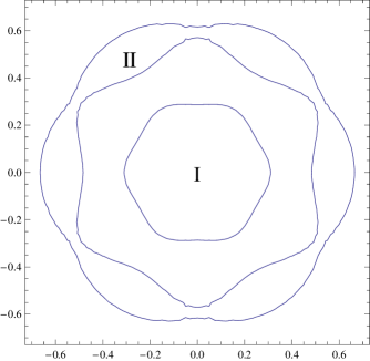
In the previous section we discussed the dispersion relations of holon and doublon excitations and the interaction between them. If momentum is measured from the center of the pockets, the holon pocket is a sphere centered at , while the doublon pockets are three ellipses centered at , long axes of which are to each other. Since the system is neutral, the area of the holon pocket is three times larger than the area of each doublon pocket. However, the long axis of doublon pockets can still be longer than the radius of holon pocket if the aspect ratio of doublon pockets is greater than 3:1. Therefore there can still be pairing at the places where the two Fermi surfaces are close. Between holon and one type of doublon the pairing is only good in one direction, but if the holon is paired with both three types of doublon, there is a good pairing in three directions, which covers a large portion of the Fermi surface. We will see that this mismatch in Fermi surfaces lead to a richer phase diagram compared to the normal-superconducting problem.
Since all the pockets are centered at (when momentum is measured from the minimums of pockets), we assume that the exciton pairs also have total momentum . In other words, it is not a LLFO state in which smaller pocket is shifted toward the edge of larger pocket. Therefore we have three pairing order parameters between holon and each type of doublon
| (46) |
Note, that the pairing is -wave because the interaction (45) only has -wave component.
According to this order parameter, the mean field decomposition of the interaction (45) is
| (47) |
Combining this with the kinetic energy in Eq. (34) and the chemical potential, the full Hamiltonian is
| (48) |
This Hamiltonian can be diagonalized using the Bogoliubov transformation. First, write Eq. (48) in the matrix form:
| (49) |
where
| (50) |
| (51) |
A Bogoliubov transformation is then a unitary transformation
| (52) |
that diagonalizes the matrix . With the new quasiparticle operators , the Hamiltonian is diagonalized as
| (53) |
where are the four components of , and are the four eigenvalues of the matrix . Therefore in the ground state, the state of quasiparticle is filled if , or empty if . The ground state energy is
| (54) |
Becuase the three doublon pockets are identical, we assume that the absolute values of the order parameters are the same for three pockets. Therefore the pairing order parameters can be characterized by one absolute value and three phases.
| (55) |
After we have made the approximation that only excitations near the minimums of the pockets are considered, the kinetic energy (34) and interaction energy (45) has the symmetry for changing the phases of three doublons independently. Therefore the mean field energy (48) does not depend on the phases of order parameters . In other words, for this simplified Hamiltonian, a state with order parameter in Eq. (46) breaks the symmetry spontaneously, and the states with different phases are degenerate. We will see in the next section that this degeneracy is lifted once we add the other parts of Coulomb interaction back.
With this degeneracy, the ground state energy in Eq. (54) only depends on the absolute value of . The ground state is obtained by minimizing the ground state energy with respect to order parameter . The results are described below
When is large and positive, the system is in an insulating phase (semiconductor phase), with no Fermi surface and . Then as the gap decreases, the system goes through a second-order phase transition at a critical value and enters a insulating phase with no Fermi surface but . In this phase the binding energy of exciton overcomes the charge gap, so there are doublon and holon excitations. However, the excitations near the Fermi surface bind into exciton, and the gap is large comparing to the Fermi energy such that the Fermi surface is fully gapped although there is a mismatch between holon and doublon Fermi surfaces. This state is an insulating phase because the charged quasiparticle is gapped. We call this phase an excitonic insulator. Then if the gap is further decreased, the system goes through a second-order phase transition at some value into a phase still with , but there are Fermi surfaces in the spectrum of quasiparticle excitation. Hence this is a conducting phase with . A typical image of the Fermi surfaces in the system is shown in Fig. 5. Eventually, the system goes through another first order phase transition at into a state with . This is a simple semimetal conducting state. A typical phase diagram for given masses and is shown in Fig. 3. For given masses, the two dimensional phase diagram for different and is shown in Fig. 4.
In phase with the excitonic condensate, the ground state has a degeneracy because of the corresponding symmetry in the simplified Hamiltonian. This degeneracy will be lifted to a degeneracy once we take into account the parts in the interaction (38) which we ignored in the dominant term approximation. In other words, the full interaction breaks symmetry, and only one is spontaneously broken.
Besides the dominant term in Eq. (41), the next leading term is the direct interaction in Eq. (39), because it is unscreened. That term can be expressed using charge density operator as
| (56) |
where is the density operator
| (57) |
In a state with translational invariance, the charge density is a constant, and vanishes at any . However, with an excitonic condensate, translational symmetry is actually broken. This can be understood by the following ways: First, in the excitonic condensate, there is pairing between holon and three types of doublon. The total momenta of these pairs are not zero: a pair of one holon and one doublon has total momentum . Therefore the translational symmetry of the system is broken. Also, one can look at the change of Brillouin zone. Originally the doublon pockets and holon pocket are at different places in the Brillouin zone. However, after the Bogoliubov transformation (52), the holon and doublon modes are mixed together. The only way this is allowed is that the Brillouin zone shrinks to one quarter of its original size, so that are all reciprocal vectors. The shrinking of Brillouin zone means that the unit cell in real space is enlarged, and the original translational symmetry is broken.
Because of the broken symmetry, we can look for non-vanishing expectation value of density operator at . Let us consider as an example. Again we consider only the excitation near the center of pockets. The expectation value of density operator is
| (58) |
In our ansatz we do not have this average put in explicitly. However, because the order parameter already breaks the , we can get a non-vanishing value for from the ansatz.
In the mean field state, the average in Eq. (58) can be calculated using the Green’s function of doublon. Consider the Green’s function matrix
| (59) |
Then according to the Hamiltonian in Eq. (49), we have
| (60) |
Then the average in Eq. (58) can be obtained by taking the inverse of the above matrix
| (61) |
Therefore the average of density operator in equation (58) is
| (62) |
The expectation value of charge density operator at the other two momenta can be evaluated similarly. Finally we get
| (63) |
It can be proved that this energy has a minimum at
| (64) |
Such a state breaks the time reversal and parity symmetry because of the complex phase, but the rotational symmetry of the original lattice is preserved. Finally from the density operator one can conclude that there is a charge order in the real space shown in Fig. 6. From the figure one can see that the unit cell is a plaque. This is consistent with the conclusion that the Brillouin zone shrinks to one quarter of its original size.
IV Fractionalized metals with topological order and Luttinger relations
The simplest route from the insulating spin liquid to a metallic state is by formation of Fermi surfaces of the holons and doublons. We can easily detect such a transition as a function of charge density and system parameters by examining the dispersion relations of the charged excitations in Eq. (12). These Fermi surfaces have quasiparticles of charge , but which are spinless. So the resulting state is not a conventional Fermi liquid, but a ‘algebraic charge liquid’ acl . The topological order of the insulator survives into the metal, and quasiparticles carry gauge charge. This section will address two related questions: what are the Luttinger relations which constrain the areas enclosed by the Fermi surfaces of this fractionalized metal, and how does this metal evolve into a Fermi liquid ?
We will examine a route to the Fermi liquid here which is similar to that considered recently by Kaul et al. acl for related states with U(1) topological order on the square lattice. We allow for the binding between the holon and doublon quasiparticles described in Section II.1, and the bosonic spinons described in Appendix A.1. This binding is mediated not by the gauge force (which is weak in the fractionalized phases we are discussing here), but by the hopping matrix element in Eq. (3). This matrix element is larger than , and so the binding force is strong. A computation of the binding force for the low energy holons/doublons and the spinons is presented in Appendix C, and position of these bound states in the Brillouin zone is illustrated in Fig. 2. The resulting bound states will have the quantum numbers of the electron operator in Eq. (2). Fermi surfaces of these ‘molecular’ bound states can also form powell , with electron-like quasiparticles which carry charge and spin 1/2. Indeed it is possible that these bound states have a lower energy than the holons or doublons, in which case the first metallic state state will not be an algebraic charge liquid (with holon/doublon Fermi surfaces), but have electron/hole Fermi surfaces leading to a ‘fractionalized Fermi liquid’ ffl1 ; ffl2 (see below and Fig. 7).
So as in Ref. acl, , the fractionalized metallic states being considered here can have a variety of distinct Fermi surfaces. As in a usual Fermi liquid, each Fermi surface can be considered to be a surface of either charge or charge quasiparticles, with the two perspectives related by a particle-hole transformation. There is also a corresponding change in the region of the Brillouin zone which is considered to be ‘inside’ the Fermi surface, and the value of the area enclosed by the Fermi surface. For convenience, let us use a perspective in which all Fermi surfaces are described in terms of charge quasiparticles, the same charge as an electron. Thus in the notation of Eqs. (28) and (29), we are considering Fermi surfaces of the , , and fermions. Let us by , , and the area of the Brillouin zone enclosed by these Fermi surfaces, divided by a phase space factor of . We are interested here in the Luttinger relations which are satisfied by these areas.
As has been discussed in Refs. powell, ; coleman, ; georges, , there is a one Luttinger relation associated with each conservation law, local or global. We have the conservation of total electronic charge which we can write as
| (65) |
where is the number of sites, and is the density of doped electrons away from half-filling i.e. the total density of electrons in the band is . There is also the local constraint associated with the Schwinger boson representation in Eq. (2)
| (66) |
A key observation is that in any state with topological order, the global conservation law associated with Eq. (66) is ‘broken’, due to the appearance of the anomalous pairing condensate . Consequentlypowell , the Luttinger relation derived from Eq. (66) does not apply in any such state.
We can now derive the constraints on the Fermi surface areas placed by the above relations using an analysis with exactly parallels that presented in Ref. powell, . We will not present any details here, but state that in the final result we simply count the contribution of each term in the conservation law by counting the number of all such particles inside every Fermi surface, whether as bare particles or as components of a molecular state. It is important in this counting to also include the number of bosons i.e. the Luttinger relation applies to bosons too powell ; coleman ; georges ; of course for the boson number counting, there is a contribution only from the fermionic molecular states. From such an analysis, after properly performing the particle-hole transformations associated with the mapping to the charge and particles, we obtain from Eq. (65) the relation
| (67) |
This relation applies in all non-superconducting phases. The corresponding relation from Eq. (66) is
| (68) |
We reiterate that Eq. (68) applies only in a state without topological order. Indeed, a state without order cannot have Fermi surfaces of fractionalized excitations, and so the only sensible solutions of Eq. (68), when it applies, are and .
With these Luttinger relations at hand, we can now describe their implications for the various phases. These phases are illustrated in Fig. 7, and described in turn below.
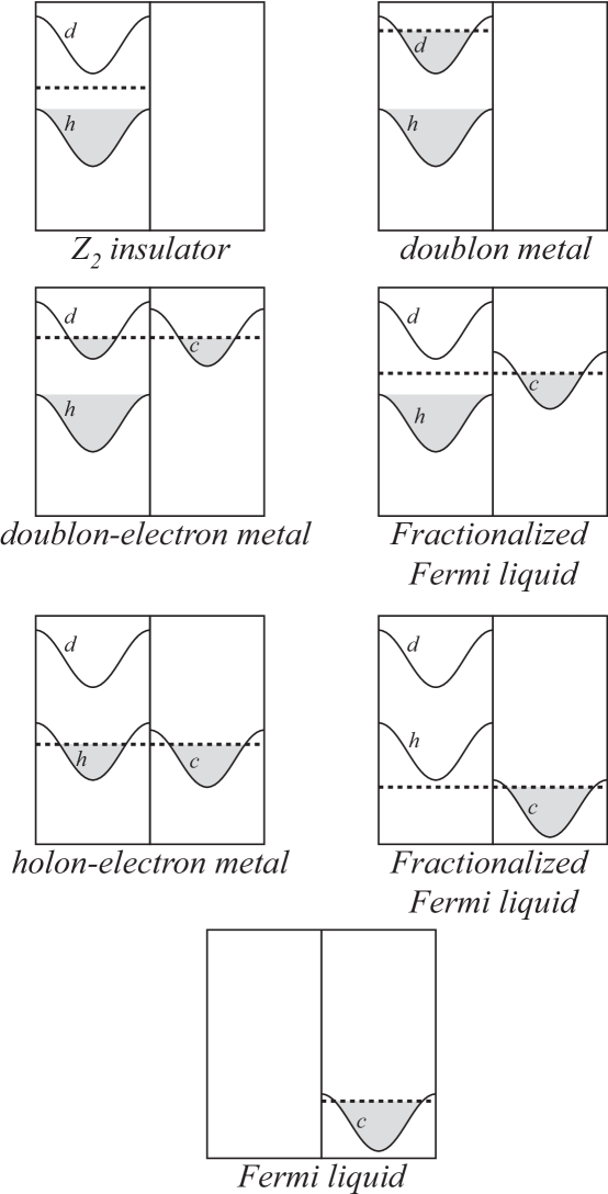
insulator:
This is the state reviewed in Appendix A. The chemical potential is within the band gap of the dispersion in Eq. (12), as shown in Fig. 7. We have , , , and , and so the relation (67) is obeyed. This relation also applies when an excitonic condensate appears: the only change is that there is mixing between the and bands.
metals:
A variety of metallic phases can appear, which are all algebraic charge liquids acl , depending upon the presence/absence of , , and Fermi surfaces, as shown in Fig. 7. All these phases have topological order, and so only the sum-rule (67) constrains the areas of the Fermi surfaces. As an example, we can dope the insulator with negative charge carriers (). This will lead to a ‘doublon metal’ with , and . As the energy of the bound state between a doublon and spinon is lowered (with increasing ), a Fermi surface of electrons can appear, leading to a state with , and . This fractionalized state with both and Fermi surfaces (a ‘doublon-electron’ metal) is the particle-hole conjugate of the ‘holon-hole’ metal discussed recently in Ref. acl, . The location of the electron Fermi surface in this metal is computed in Appendix C, and will reside at pockets around the electron dispersion minimum in Fig. 2.
Fractionalized Fermi liquid:
With a continuing increase of the doublon-spinon binding energy in the doublon-electron metal just discussed, there is a transfer of states from within the doublon Fermi surface to within the electron Fermi surface, until we reach the limiting case where . At the same time we have , and then Eq. (68) requires . So the chemical potential is in the gap between the doublon and holon bands, as shown in Fig. 7. This state is the fractionalized Fermi liquid of Refs. ffl1, ; ffl2, .
Transition to the Fermi liquid
We now continue decreasing the energy of the electron bound state, in the hopes of eventually reaching a conventional Fermi liquid. One plausible route is that illustrated in Fig. 7. As the electron energy is lowered from the fractionalized Fermi liquid, the chemical potential goes within the lower holon band, and we obtain a fractionalized holon-electron metal. Note that this state has both an electron-like Fermi surface with charge carriers (as measured by the contribution to the Hall conductivity), and a holon Fermi surface with charge carriers. Eventually, the chemical potential goes below both the holon and doublon bands (see Fig 7), and we obtain another fractionalized Fermi liquid with and . Note that this is the same area of an electron-like Fermi surface as in a conventional Fermi liquid. However, the topological order is still present, which is why we denote it ‘fractionalized’: the fractionalized holon and spinon excitations are present, but all of them have an energy gap. Eventually, however, we expect a confinement transition in the gauge theory, leading to a conventional Fermi liquid with no fractionalized excitatons. Because the Luttinger relation in (68) is saturated by the electron contribution, we expect this confinement transition will be in the universality class of the ‘even’ gauge theory, rather than the ‘odd’ gauge theory ms ; fradkin .
V Superconducting states
The projected symmetry group analysis can be extended to analyze the pairing symmetry in possible superconducting states. In a superconducting state, the pairing symmetry can be determined by the relative phases of the expectation value
| (69) |
at different directions. On the other hand, the PSG determines how the operator transforms in rotation, and consequently determines how Eq. (69) transforms when the bond is rotated to another direction. Therefore the PSG of the electron operators can determine the pairing symmetry.
In our Schwinger-boson-slave-fermion ansatz, the fermionic holon and doublon excitations form Fermi seas around the bottom of their bands. If there are appropriate attractive forces, holons and doublons will become superconducting, and the pairing of holons or doublons will make Eq. (69) nonzero because the spinon is already paired. Similarly, the pairing symmetry of holon and doublon can also be determined by their PSGs, which are related to the PSG of electron according to Eq. (2). Therefore the pairing symmetry of electrons and quasiparticles are related.
When determining the PSG of holon and doublon operators, it is assumed that the physical electron operator is invariant under symmetry transformations. However, in the superconducting state the gauge symmetry of electron is broken and the electron operator may need a gauge transform after a lattice symmetry operation to recover. The pairing pattern is directly related to the gauge transform associated with rotation. Assume that the electron operator transforms in the following way after a operation:
| (70) |
Then after the rotation the superconducting order parameter (69) becomes
| (71) |
This equation shows the pairing type of the superconducting state.
If we want a superconducting state with translational and rotational symmetries, the order parameter (69) should recover after acting three times. This requires the phase satisfies
| (72) |
which implies that . It is easy to see that these choices correspond to -wave and pairing patterns. (Note, that the -wave pairing breaks time reversal symmetry).
On the other hand, Eq. (70) also determines the PSG of holons and doublons, and therefore determines their pairing patterns. For the pairing, the result is in Table 3:
| Particle | Pairing symmetry | |
|---|---|---|
| -wave | ||
| -wave | ||
| -wave | ||
| -wave | ||
| -wave |
For the -wave pairing, the result is in Table 4:
| Particle | Pairing symmetry | |
|---|---|---|
| -wave | ||
| -wave | ||
| -wave | ||
| -wave | ||
| -wave |
From Table 3 and 4 we can see that -wave pairing of holon and doublon will result in -wave pairing of electron; -wave pairing of holon and doublon will result in -wave pairing of electron. In the rest of this section we will show that the interaction mediated by spinon excitation leads to a -wave pairing symmetry for holon and doublon, and results in a -wave pairing for electron.
In the spin liquid state, the excitation of spin degree of freedom is described as Schwinger boson. The holon acquires a kinetic energy from the original hopping term by replacing the product of spinon operators by the mean field average. Moreover, beyond the mean field theory this term also describes interaction between holon and spinon excitations. This type of interaction results in an interaction between two holons by exchanging a pair of spinons. Detailed calculation will show that this interaction is attractive and can lead to superconducting pairing of fermionic holons.
In Appendix B, we calculate the scattering amplitude between two holons by exchanging two spinons shown in Fig. 8. Also, a contribution from fluctuation of spinon mean field solution is included to make the result consistent with the constraint that there is one spinon on every site.
interact-fmf {fmfgraph*}(160,160) \fmfpenthin \fmfbottomi1,i2 \fmftopo3,o4 \fmffermion,label=i1,v1 \fmffermion,label=v1,o3 \fmffermion,label=i2,v2 \fmffermion,label=v2,o4 \fmfdashes,label=,leftv1,v2 \fmfdashes,label=,rightv1,v2 \fmfdotv1,v2
The scattering between two holons by exchanging two spinons can be represented as a Feynman diagram in Fig. 8. The vertex in this figure comes from the hopping term in equation (3). For Cooper pairing instability, we are interested in the following situation: the incoming and outgoing momenta are on the Fermi surface; the total incoming and outgoing momenta are zero; the energies of incoming and outgoing particles are on shell. Therefore the interaction is a function of the angle between incoming and outgoing fermions. In Appendix B, we calculate the scattering amplitude of this Feynman diagram. Also, a contribution from fluctuation of spinon mean field solution is included to make the result consistent with the constraint that there is one spinon on every site. The result is the following
When , we get
| (73) |
When , we get
| (74) |
where is a UV cutoff of the system, is the spinon gap, and is the momentum transfered in the interaction.
Since the incoming and outgoing particles are fermions, we need to antisymmetrized :
| (75) |
The antisymmetrized interaction in the limit of equation (73) is proportional to , and therefore has only -wave component. The antisymmetrized interaction for the other limit (Eq. (74)) is a mixture of odd-parity wave components, but the -wave component is dominant. Consequently this interaction will lead to a -wave superconducting instability for holon, and result in a -wave pairing superconducting state in terms of electron according to table 3.
VI Conclusions
This paper has presented a route for the transition from an insulator to a metal for electrons on a triangular lattice. Our primary purpose was to pay close attention to the antiferromagnetic exchange interactions, and the consequent resonating valence bond (RVB) correlations in the insulator. We were particular interested in the fate of these RVB correlations in the metal. Our approach borrows from a recent theory acl of ‘algebraic charge liquids’ (ACL), and can be straightforwardly generalized to other lattices in both two and three dimensions. As we noted in Section I, our theory of the insulator-to-metal transition is complementary to the DMFT theory dmft of the metal-to-insulator transition. The latter begins with a theory of the correlated Fermi liquid, but pays scant attention to RVB correlations, which we believe are particularly important on the triangular lattice.
We have introduced a variety of intermediate phases in the route from the insulator to the metal, and so we now present a brief review of their basic characteristics.
First, let us discuss the possible phases of the insulator and their charged excitations. We used a spin liquid state sstri ; ashvin with bosonic spinons as a central point of reference. This state was reviewed in Appendix A, and its low energy excitations are gapped neutral spinons which are located (in our gauge choice) at points in the Brillouin zone shown in Fig. 2. Its charged excitations consist of spinless, charge holons , and charge doublons , which were described in Section II; their positions in the Brillouin zone (in our gauge choice) are also in Fig. 2. We also discussed, Appendix C the binding of holons/doublons with spinons to form charged, excitations which are hole/electron-like; the location of these bound states in the Brillouin zone is indicated in Fig 2. This binding binding between gapped excitations is caused by the term in the - model, and so the attractive force is quite strong. Consequently, it may well be that the lowest charged excitations of a spin liquid are electrons and holes, and not doublons and holons. Note that the binding is present already in the deconfined spin-liquid state, and is quite distinct from the confinement transition.
Although, we did not say much about this explicitly, our analysis of excitations in the spin liquid is easily continued into confining insulators with Néel or VBS order. The transition into the Néel state is driven by the condensation of the spinons, as described in Ref. css, . The charged excitations in the Néel state are simple continuations of the holons and doublons in the spin liquid, as has been discussed in some detail previously for the square lattice ribhu1 . The charged excitations in the VBS state will be the electrons and holes described in Appendix C.
Continuing our discussion of insulating states, our primary new result was the prediction of an insulator with an excitonic condensate in Section III. We described the excitonic instability starting from the spin liquid, mainly because this led to the simplest technical analysis. However, we expect very similar excitonic instabilities to appear also from the Néel and VBS insulators. One physical manifestation of the excitonic instability was a breaking of the space group symmetry of triangular lattice. In our mean-field analysis we found the translational symmetry breaking depicted in Fig. 6, which serves as a test of our theory.
Moving onto metallic states, we found a plethora of possibilities depending upon precisely which instabilities of the insulator was present (Néel, VBS, excitonic), and which of the charged excitations of the insulator had the lowest energy (holon, doublon, hole, electron). Some of these states were algebraic charge liquids, while others were Fermi liquids. However, the Fermi surface areas in all these states satisfied either the conventional Luttinger relation, or a modified Luttinger relations, and these were discussed in Section IV.
Finally, we also considered the onset of superconductivity due to pairing of like-charge fermions in Section V. Again, for technical reasons, it was simplest to describe this instability using the holon/doublon excitations of the spin liquid, but similar results are expected from instabilities of the other states.
The possible experimental applications of our results to organic compounds was already discussed in Section I and so we will not repeat the discussion here. Here we only reiterate that our model for -(ET)2Cu2(CN)3 is a spin liquid, close or across its transition to a state with Néel order, with an excitonic instability at low temperatures.
Acknowledgements.
We thank K. Kanoda, Sung-Sik Lee, and T. Senthil for useful discussions. This work was supported by NSF Grant No. DMR-0537077.Appendix A spin liquid
Consider the model on a triangle lattice with anti-ferromagnetic interaction between nearest neighbor sites.
| (76) |
We use the coordinates system labeled in Fig. 1. and the Schwinger-boson mean field ansatz with the following ground state expectation values:
| (77) |
where is Schwinger boson operator.
| (78) |
The ansatz (77) stays the same if both the spinon operators and and parameters are transformed under the following gauge transformation
| (79) |
Because of this gauge freedom, ansatz with different and configurations may be equivalent after a certain gauge transform. Therefore the symmetry of and fields may be smaller than the symmetry of the ansatz. In particular, we consider the symmetry group of the triangle lattice. (We only consider ansatz that does not break the lattice symmetry). When a group element acts on the ansatz, an associated gauge transform may be required for the and fields to recover. This gauge transform forms the PSG. According to equation (79), gauge transform can be defined using the phases . Consequently the PSG can also be specified using phases of the gauge transformations. The phases of the gauge transform associated with symmetry group element is denoted by .
For triangle lattice, the lattice symmetry group can be generated by four elements: and , which are the translations along the 1 and 2 direction; , which is the rotation of ; , which is the reflection operation respect to the axis. In the coordinates system used in this note, these elements can be represented as
| (80) |
It can be proved that there are two possibilities for PSG of 2D triangle lattice. We are interested in one of them, which is called “zero-flux” ansatz. The zero-flux PSG can be described as
| (81) |
These are also shown in Table 5.
Assume that the system is slightly doped with holes with hole concentration . Hence the spinon state is not changed. We describe the system by introducing fermionic holon
| (82) |
where is the electron and is holon operator. To preserve the physical electron operator, the holon needs to transform as follows in the gauge transformation (79)
| (83) |
The PSG of holon is summarized in the second row of table 5.
| Operator/Field | ||||
|---|---|---|---|---|
The PSG of spinon operators (81) determines how and transforms under lattice symmetry operations, and therefore reduces the degree of freedom of parameters in the ansatz to only two free ones. implies that the ansatz is translational invariant. By definition and has the following properties
| (84) |
Therefore and determines the structure of the ansatz: is the same real number on every bond; , and the sign is shown in Fig. 9.

A.1 Low energy theory of spinons
In this section we analyze low energy excitations of spinon.
For spinon Hamiltonian, if we take the mean field decomposition of Eq. (76) using parameters (77), the result is
| (85) |
where
| (86) |
Plug in the “zero-flux” type of ansatz and write the Hamiltonian in momentum space, we get
The mean field Hamiltonian (87) can be diagonalized using Bogoliubov transformation
| (90) |
After diagonalizing the Hamiltonian (89) becomes
| (91) |
The spectrum of the quasi-particle is
| (92) |
The coefficients in Bogoliubov transformation and , which diagonalize the Hamiltonian, are
| (93) |
Then it is easy to see that
| (94) |
It can be shown that the above spectrum has two minimums at , where .
To describe the low energy excitation of spinon degree of freedom, the quasi-particle can be used. Consequently we are interested in its PSG. Usually the symmetry transforms are described in coordinate space rather than momentum space. Therefore consider the Fourier transformation of operator at a certain momentum
| (95) |
Since the low energy excitations are near , two new field operators are defined as
| (96) |
Another way of describing the low energy excitations of spinon field is to use two complex variables and , which can also be used as order parameters in the spin ordered phase.
To begin with, fields are introduced by discussing the ordered phase. The excitation spectrum (92) has two minimums at . When becomes larger and larger the gap at these two momenta vanishes. Consequently the quasi-particle modes at these momenta will condense and form long range antiferromagnetic order.
In the spin ordered state, spinon field condensates in the following wayashvin :
| (99) |
where and are the same fields as and in Ref. ashvin, . In antiferromagnetic ordered phase, they acquires non-zero expectation values. However, in spin liquid phase they represent gapped excitations.
From Eq. (99) one can solve in terms of spinon operators
| (100) |
Actually the operators and fields are correlated to each other: they become the same thing when the system is close to the critical point between spin liquid phase and antiferromagnetic long range order phase. To see this, consider only the long wavelength component in Eq. (96). When , we can take the approximation , . Therefore becomes
Note, that
and similarly
The operator can be simplified as
| (101) |
Similarly for
| (102) |
(We used Eq. (94).)
Appendix B Interaction mediated by spinon excitation
In this section we calculated the interaction between holon or doublon through exchanging two spinon excitations described in section V.
First, consider the interaction between two holons. The interaction is shown in Fig. 8, in which the interaction vertex between holons and spinons comes from the hopping term in equation (3). When the spinon gap is small comparing to the band width of spinon, the low energy spinon excitation can be described by the and complex fields defined in equation (100). In terms of field, the interaction is
in which the terms involve high momentum transfers like are ignored. After a Fourier transform one get from the above equation
| (105) |
where is a complex number .
Here we are interested in the situation that both the spinon gap and the doping are small. When the spinon gap is small, the interaction is dominated by the spinon excitations near the bottom of the minimum of spinon band. When the doping is small, the Fermi surface is also small, so that the momentum of fermions in the interaction vertex is also small. When all the momenta in the interaction vertex are small, the function in the vertex can be expanded as
| (106) |
where is the lattice constant. The leading order in the expansion is a constant, which corresponds to a contact interaction.
When the gap is small, the two fields describes bosonic spinon excitations in the vicinities of momenta . The two branches of excitations has the same dispersion relation
| (107) |
where is the spinon gap and is the spin wave velocity. The propagator of fields can be worked out from the spinon mean field Hamiltonian (87) through the relation between the two representations. The result shows bosonic excitations with the above dispersion relation and a spectrum weight determined by the order parameters of the spinon ansatz.
| (108) |
where the spectrum weight
| (109) |
Similarly the Green’s function of field can be obtained. The result is the same as Eq. (108).
Using the interaction vertex (105) and the Green’s function (108) for fields, the Feynman diagram Fig. 8 can be evaluated. To the leading order in Eq. (106),
| (110) |
The integral and frequency summation can be worked out at as in Ref. sachdev1999qpt,
| (111) |
When the momenta in the interaction are all small, this is the result in the leading order. However, if the constraint of the complex fields in Eq. (113) is taken into account, the contact interaction should give no contribution to the holon scattering process because the spinon fields appears in the interaction can be simply replaced by the constant 1. However, in the above equation we do get a contribution to the scattering amplitude from that contact interaction. The reason is that we use a large expansion (or mean field approximation) in determining the low energy excitation of the spinon field. However, in such an expansion the constraint (113) is replaced by a global chemical potential. Therefore to correctly include the effect of the constraint we have to take into account the order fluctuation of the chemical potential field.
The original action of the fields is a non-linear sigma model.
| (112) |
with the constraint
| (113) |
The partition function of this action is
| (114) |
where in our case . In the above action, the delta function that enforces the constraint (113) can be replaced by a Lagrangian multiplier field as follows
| (115) |
Integrate out the field and take the large limit, one can get the saddle point of field as , where the mass is determined by the following mean field self-consistent Eq. (see Eq. (5.21) in Ref. sachdev1999qpt )
| (116) |
To calculate the correction in the order, the fluctuation of field needs to be included. Section 7.2 of Ref. sachdev1999qpt calculated that the propagator of field is , where is the bare density-density correlation function of fields:
| (117) |
If the fluctuation of field is included, there will be another Feynman diagram in addition to Fig. 8 (see Fig. 10).
interact-lambda {fmfgraph*}(160,160) \fmfpenthin \fmfbottomi1,i2 \fmftopo3,o4 \fmffermion,label=i1,v1 \fmffermion,label=o3,v1 \fmffermion,label=i2,v2 \fmffermion,label=o4,v2 \fmfdashes,leftv1,vv1 \fmfdashes,rightv1,vv1 \fmfdbl_dashesvv1,vv2 \fmfdashes,leftvv2,v2 \fmfdashes,rightvv2,v2 \fmfdotv1,v2
The contribution from this diagram is
| (118) |
Therefore it cancels the contribution from Fig. 8. This is consistent with the constraint (113), and it implies that there is no holon-holon scattering coming from the contact interaction. Consequently we need to consider interaction with momentum dependence. Taking the next order in interaction (105), one will get
| (119) |
where the order gives no contribution to holon-holon interaction because of the constraint, and therefore can be dropped.
Plug in the interaction in Eq. (118), the holon-holon interaction shown in Fig. 8 and Fig. 10 becomes
| (120) |
Let , and replace by , Eq. (120) can be simplified as
| (121) |
It is easy to prove that the terms involving are canceled. Therefore the interaction coefficient can be written as
| (122) |
The factor in the integral introduces an UV divergent. The most divergent term in the integral is proportional to , where the cut-off . However, the most divergent term does not depend on and and will be canceled out when including the contribution from switching the two outgoing fermions. Therefore the relevant leading order is . Combine that with the prefactor , we conclude that
| (123) |
The dimensionality of is (see equation (111). Therefore should be proportional to the larger one of and when one is much larger than the other. Consequently by dimensional analysis we can get the results summarized in Eq. (73) and (74).
Then let us consider the counterpart of this interaction for doublon excitations. This can be done in the same way as the holon interactions, while the only difference is that low-energy doublon excitations are around non-zero momenta : , and .
We start with the second term in the hopping Hamiltonian (3). In the limit of small doping and small spinon gap, we can again replace the operators by fields. After a Fourier transform the interaction vertex becomes
| (124) |
Low energy doublon excitations are located in the vicinities of the minimums in the doublon band . To calculate the interaction between doublons, we need to replace the operator in the above Hamiltonian with the operator defined in Eq. (19). Then Eq. (124) becomes
| (125) |
Note, that we only included interaction between the same type of doublon, because interaction between two different types of doublon cannot be mediated by spinons near the minimum of spinon band, and therefore is much smaller.
With this interaction vertex and the same Green’s function of fields we got before in Eq. (108), we can evaluate the Feynman diagram Fig. 8 with incoming and outgoing type- doublons together with correction in Fig. 10. The result has the same form as we have in Eq. (73) and (74) because the interaction vertex (125) has the same form as the one for holons (105).
Appendix C Bound state of spinon and holon
One spinon and one holon may form a bound state if we take into account the interaction between the two due to the hopping term in Eq. (3). Again, we need to include the effect of constraint (113); in other words, we need to consider the contribution from the fluctuation of field shown in Fig. 10.
In general, we consider the interaction between two holons and two spinons with incoming and outgoing momenta shown in Fig. 11.
bound-tree {fmfgraph*}(100,100) \fmflefth1,h2 \fmfrights1,s2 \fmffermion,label=h1,v1 \fmffermion,label=v1,h2 \fmfscalar,label=v1,s2 \fmfscalar,label=s1,v1 \fmfdotv1
The tree level interaction coming from the hopping term in equation (105) has the momentum dependence according to the expansion (106)
| (126) |
Therefore the interaction vertex at tree level is
| (127) |
For the same reason we gave in Appendix B, the one loop correction due to the fluctuation of field needs to be combined with the zero-th order contribution from equation 126. This is represented by Fig. 12 and is expressed by the following equation
bound-oneloop {fmfgraph*}(300,100) \fmflefth1,h2 \fmfrights1,s2 \fmffermion,label=h1,v1 \fmffermion,label=v1,h2 \fmfscalar,left, label=v1,v3 \fmfscalar,left, label=v3,v1 \fmfdbl_dashes, label=v3,v2 \fmfscalar,label=v2,s2 \fmfscalar,label=s1,v2 \fmfdotv1 \fmfdotv2
| (128) |
where the interaction depends on the incoming momentum , momentum transfer and energy transfer .
Add the two contributions in Eq. (127) and (128) together, one immediately see that the terms not depend on and in equation (127) will be canceled by corresponding terms in the other term, due to the definition of in equation (117). This yields to the following result
| (129) |
It is easy to see that in Eq. (129), the interaction can be seperated into two parts: the first term is a simple one but with a dependence on , which does not appear in usual two-body interactions; the second one is the result of a loop integral and only depends on the transfered momentum and energy.
The asymptotic behaviors of the second term in and can be studied by the same dimension analysis method used in Appendix B. By counting the power of in the loop integral one can see that the most divergent term is proportional to , and the term in the next order does not depend on . However, unlike the case in equation (122), here the divergent term does give a and dependent interaction because of the prefactor. Therefore the dominant term in equation (129) is
| (130) |
The bound state problem can be solved by solving Bethe-Salpeter equationSalpeter1951 . In order to see the qualitative results of the binding potential in Eq. (130) we ignored the frequency dependence and assume that the dispersion relations of holon and spinon are both non-relativistic. In this case the Bethe-Salpeter equation for the relative motion is
| (131) |
where is the relative momentum; is the reduced mass in center of mass frame; is the bound state energy; is the total momentum in the center of mass frame; is the wave function of relative motion in the momentum space. Numerical calculation shows that there can be one or more bound states due to the interaction (130).
In general, the interaction depends on both the relative momentum , and the total momentum . However, the dominant term (130) only depends on . Moreover, although the full interaction (129) depends on all momenta, the dependence on can be separated
| (132) |
Therefore the motion of the center of mass can still be separated from the relative motion, and the bound state energy can be written as
| (133) |
where is the bound state energy which does not depend on , and , are masses of holon and spinon respectively. Consequently the bound states have minimal energy at . Since the momenta we use in this Appendix are all measured from the center of spinon and holon energy minimums, the position of the bound state energy minimum is the sum of holon and spinon minimums. The former is at the origin; the later is at . Therefore the position of bound state minimums is also . This is shown in Fig. 2
For doublons, we can also get an attractive interaction between them and spinon from Eq. (125). Because of the same dimension analysis argument the interaction has the same form as (130). Therefore, the bound state of doublon and spinon, or electron excitation locates at the sum of momenta of doublon and spinon, which is also shown in Fig. 2.
References
- (1) K. Miyagawa, A. Kawamoto, Y. Nakazawa, and K. Kanoda, Phys. Rev. Lett. 75, 1174 (1995).
- (2) M. Tamura, A. Nakao, and R. Kato, J. Phys. Soc. Japan 75, 093701 (2006).
- (3) Y. Ishi, M. Tamura, and R. Kato, J. Phys. Soc. Japan 76, 033704 (2007).
- (4) Y. Shimizu, H. Akimoto, H. Tsujii, A. Tajima, and R. Kato, cond-mat/0612545.
- (5) Y. Shimizu, K. Miyagawa, K. Kanoda, M. Maesato, and G. Saito, Phys. Rev. Lett. 91, 107001 (2003).
- (6) Y. Shimizu, K. Miyagawa, K. Kanoda, M. Maesato, and G. Saito, Phys. Rev. B 73, 140407 (2006).
- (7) S.-S. Lee, P. A. Lee, and T. Senthil, Phys. Rev. Lett. 98, 067006 (2007).
- (8) R. R. Singh and D. A. Huse, Phys. Rev. Lett. 68, 1766 (1992).
- (9) G. Misguich, C. Lhuillier, B. Bernu, and C. Waldtmann, Phys. Rev. B 60 1064 (1999).
- (10) O. I. Motrunich, Phys. Rev. B 72, 045105 (2005).
- (11) P. Sahebsara and D. Sénéchal, arXiv:0711:0244.
- (12) S. Sachdev, Phys. Rev. B 45, 12377 (1992).
- (13) F. Wang and A. Vishwanath, Phys. Rev. B 74, 174423 (2006).
- (14) A. V. Chubukov, T. Senthil and S. Sachdev, Phys. Rev. Lett. 72, 2089 (1994).
- (15) R. Moessner and S. L. Sondhi, Phys. Rev. B 63, 224401 (2001).
- (16) A. Georges, G. Kotliar, W. Krauth, and M. J. Rozenberg, Rev. Mod. Phys. 68, 13 (1996).
- (17) B. J. Powell and R. H. McKenzie, J. Phys.: Condens. Matter 18, R827 (2006).
- (18) M. Hermele, Phys. Rev. B 76, 035125 (2007).
- (19) B. I. Halperin and T. M. Rice, Solid State Physics 21, 115 (1968).
- (20) I. Kezsmarki, K. Kanoda, et al., unpublished.
- (21) I. Kezsmarki, Y. Shimizu, G. Mihaly, Y. Tokura, K. Kanoda, and G. Saito, Phys. Rev. B 74, 201101 (2006).
- (22) R. K. Kaul, Y. B. Kim, S. Sachdev, and T. Senthil, Nature Physics to appear, arXiv:0706.2187.
- (23) X.-G. Wen, Phys. Rev. B 65, 165113 (2002).
- (24) Z. Zou and P. W. Anderson, Phys. Rev. B 37, 627 (1988).
- (25) S. Powell, S. Sachdev, and H. P. Büchler, Phys. Rev. B 72, 024534 (2005).
- (26) T. Senthil, S. Sachdev, and M. Vojta, Phys. Rev. Lett. 90, 216403 (2003).
- (27) T. Senthil, M. Vojta, and S. Sachdev, Phys. Rev. B 69, 035111 (2004).
- (28) P. Coleman, I. Paul, and J. Rech, Phys. Rev. B 72, 094430 (2005).
- (29) O. Parcollet, A. Georges, G. Kotliar, and A. Sengupta, Phys. Rev. B 58, 3794 (1998).
- (30) R. Moessner, S. L. Sondhi, and E. Fradkin, Phys. Rev. B 65, 024504 (2002).
- (31) R. K. Kaul, A. Kolezhuk, M. Levin, S. Sachdev, and T. Senthil, Phys. Rev. B 75, 235122 (2007).
- (32) E. E. Salpeter and H. A. Bethe, Phys. Rev. 84, 1232 (1951).
- (33) S. Sachdev. Quantum Phase Transitions. Cambridge University Press, 1999.