The non-equilibrium response of the critical Ising model: Universal scaling properties and Local Scale Invariance

Abstract

Motivated by recent numerical findings [M. Henkel, T. Enss, and M. Pleimling, J. Phys. A: Math. Gen. 39 (2006) L589] we re-examine via Monte Carlo simulations the linear response function of the two-dimensional Ising model with Glauber dynamics quenched to the critical point. At variance with the results of Henkel et al., we detect discrepancies between the actual scaling behavior of the response function and the prediction of Local Scale Invariance. Such differences are clearly visible in the impulse autoresponse function, whereas they are drastically reduced in integrated response functions. Accordingly, the scaling form predicted on the basis of Local Scale Invariance simply provides an accurate fitting form for some quantities but cannot be considered to be exact.

I Introduction

The non-equilibrium collective relaxation of pure systems quenched at or below their critical points has been recently the subject of a renewed interest in connection with the fact that two-time quantities — such as response and correlation functions — display a scaling behavior similar to the one observed in glassy systems Cugliandolo ; God-rev ; cg-rev . In addition, at the critical point, this scaling behavior is characterized by a certain degree of universality God-rev ; cg-rev which renders it largely independent of the microscopic details of the systems and allows its investigation via suitable minimal models, either on the lattice or in the continuum. The former can be easily studied via Monte Carlo simulations (or, in a limited number of cases, exact solutions are available), whereas powerful field-theoretical methods have been developed for the latter.

In what follows we will be concerned with the behavior of the two-time response function. Consider a lattice model characterized by degrees of freedom $\sigma_{\bf x}$ with ${\bf x}\in{\mathbb{Z}}^{d}$, interacting via an Hamiltonian ${\mathcal{H}}[\{\sigma_{\bf x}\};\{h_{\bf x}(t)\}]={\mathcal{H}}_{0}[\{\sigma_{\bf x}\}]-\sum_{\bf x}\sigma_{\bf x}h_{\bf x}(t)$, where $h_{\bf x}(t)$ is a time-dependent external field. In the case of the Ising model $\sigma_{\bf x}=\pm 1$, ${\mathcal{H}}_{0}[\{\sigma_{\bf x}\}]=-J\sum_{\langle{\bf x}{\bf y}\rangle}\sigma_{\bf x}\sigma_{\bf y}$ ($J>0$), the sum being over pairs $\langle{\bf x}{\bf y}\rangle$ of nearest neighboring sites. The stochastic dynamics of the model, due to the coupling to a thermal bath of temperature $T$, can be implemented according to different rules and yields a time dependence of the value of the local degree of freedom $\sigma_{\bf x}(t)$. The linear two-time response function is defined as

$$R_{r}(t,s)=\left.\frac{\delta\langle\sigma_{\bf x}(t)\rangle}{\delta h_{\bf y}(s)}\right|_{h=0}$$ (1)

where $r=|{\bf x}-{\bf y}|$, $\langle\ldots\rangle$ indicates the average over the possible realizations of the stochastic dynamics, and invariance under space translations has been assumed. Causality implies that $R_{r}(t,s)$ vanishes for $s>t$ and therefore we shall assume $t>s$ in what follows. In addition, we shall primarily consider the local response function (also referred to as autoresponse function)

$$R(t,s)\equiv R_{r=0}(t,s).$$ (2)

If the system is in thermal equilibrium with the bath, the dynamics is invariant under time translations and therefore $R_{r}(t,s)$ actually depends only on $\tau\equiv t-s$, i.e., $R_{r}(t,s)=R_{r}^{\rm(eq)}(\tau;T)$. Time-translational invariance is naturally broken if, at time $t=0$, the temperature of the bath is suddenly changed from an initial value $T_{\rm i}$ — which we shall assume to be high enough to yield a disordered state in the system — to a final value $T_{\rm f}\neq T_{\rm i}$. After the quench, the system undergoes a non-equilibrium relaxation towards the new equilibrium state at the temperature $T_{\rm f}$, which is attained after a time $t_{\rm eq}$. In some circumstances, however, $t_{\rm eq}=\infty$ and the dynamics retains its non-equilibrium character forever. Interestingly enough, a robust scaling behavior emerge in this regime as it is revealed by two-time quantities such as the linear response function (1). In the paradigmatic case of ferromagnetic systems, $t_{\rm eq}=\infty$ — in the thermodynamic limit — if the quench occurs at $T_{\rm f}\leq T_{c}$, where $T_{c}$ is the critical temperature of the system. In such a case, the behavior of $R_{r}(t,s)$ depends on the relation between $t$ and $s$. We restrict our analysis to the case $s,\tau\gg{\tau_{\rm micr}}$, where ${\tau_{\rm micr}}$ is a microscopic time scale set by the dynamics and such that for $s,\tau<{\tau_{\rm micr}}$ non-universal corrections to scaling appear. In the sector $s\gg\tau\gg{\tau_{\rm micr}}$, referred to as short-time separation regime (STSR), time-translational invariance and time-reversal symmetry are recovered in local quantities, resulting in an equilibrium-like dynamics:

$$R(t,s)=R^{\rm(eq)}(\tau;T_{\rm f}).$$ (3)

This quasi-equilibrium behavior is quite generally expected in systems with slow dynamics (see, e.g., Refs. Cugliandolo ; God-rev ; cg-rev ). By contrast, for $s\gg{\tau_{\rm micr}}$ and fixed $u\equiv t/s>1$, referred to as aging regime, one expects the scaling behavior

$$R(t,s)=R^{\rm(ag)}(t,s)=s^{-1-a}F_{R}(u)\;,$$ (4)

which is characterized by the scaling function $F_{R}$ and the exponent $a$. These being the behaviors in two different regimes, it remains to be clarified: (a) how the crossover between the forms (3) and (4) actually occurs in $R(t,s)$ and (b) how $F_{R}(u)$ behaves.

For quenches at the critical temperature these issues can be addressed via scaling arguments God2 ; God-rev and the renormalization-group (RG) approach JSS , which yield

$$R(t,s)=A_{R}s^{-1-a}u^{\theta}(u-1)^{-1-a}f_{R}(u)$$ (5)

where the exponent $a$ is related to the usual static and dynamic critical exponents $\eta$ and $z$ by

$$a=\frac{d-2+\eta}{z},$$ (6)

$\theta$ is the so-called initial-slip exponent JSS , $A_{R}$ is a non-universal constant (fixed by the condition $f_{R}(u\gg 1)=1$) and $f_{R}(u)$ is a universal scaling function such that nota1

$$f_{R}(1^{+})\neq 0\quad\mbox{and}\quad\mbox{{\it finite}}.$$ (7)

$f_{R}(u)$ can be calculated by means of a variety of field-theoretical techniques. As a consequence of Eq. (7), Eq. (5) can be cast in the form

$$R(t,s)=R^{\rm(eq)}(\tau;T_{c})R^{\rm(off)}(u)$$ (8)

where

$$R^{\rm(eq)}(\tau;T_{c})=B_{R}\tau^{-1-a}$$ (9)

is the equilibrium critical response function with $B_{R}=A_{R}f_{R}(1^{+})$ and

$$R^{\rm(off)}(u)=u^{\theta}f_{R}(u)/f_{R}(1^{+})$$ (10)

is the non-equilibrium contribution. In the STSR $R^{\rm(off)}(u)\simeq 1$ and the response function (5) reduces to the form (9), in agreement with what expected from Eq. (3). In the aging regime $R^{\rm(off)}(u)\neq 1$ and the invariance under time-translations, typical of equilibrium, is broken. Equation (8) shows that in the quench at $T_{\rm f}=T_{c}$ the crossover between the quasi-equilibrium $R^{\rm(eq)}$ and the aging $R^{\rm(ag)}$ behavior occurs multiplicatively via the factor $R^{\rm(off)}$.

Unfortunately, no equivalent powerful methods are available for the analytical investigation of the behavior of the response function after a quench to $T_{\rm f}<T_{c}$. Nonetheless, the available numerical simulations of the Ising model noiTRM ; noiRd2 ; noi , the exact results for the Glauber-Ising chain God1 ; Lippiello quenched to $T_{\rm f}=0$ footnote1d , and the predictions of approximate theories of phase-ordering berthier ; EPJ ; Mazenko suggest that the response function for scalar systems in the aging regime can be cast in the form of Eq. (5) where $a$ is a scaling exponent whose behavior has been investigated in Refs. noiTRM ; noia , with

$$f_{R}(u)=(u-1)^{1/z_{g}}\;.$$ (11)

(See, however, Refs. MHenkel ; Janke where $f_{R}(u)\equiv 1$ has been numerically inferred by looking at the so-called thermoremanent magnetization — $\chi(t,[0,s])$ and $\hat{\chi}_{k=0}(t,[0,s])$, see Eqs. (18) and (19) below — for the Ising, $3$- and $8$-state Potts models.) Here $z_{g}$ is the growth exponent which controls the time-evolution of the typical domain size $L(t)\sim t^{1/z_{g}}$ in systems with discrete symmetries (e.g., $z_{g}=2$ for the Ising model with Glauber dynamics) Bray . Note that, at variance with the prediction of the scaling and RG analysis for the quench to $T_{\rm f}=T_{c}$, $f_{R}(u)$ vanishes for $u\rightarrow 1^{+}$. Let us stress that, while for $T_{\rm f}=T_{c}$ scaling arguments and RG approach predict Eq. (5) to be obeyed for every $t$ and $s$, for $T_{\rm f}<T_{c}$ this expression holds only in the aging regime.

Due to the lack of general predictions for the scaling function $f_{R}(u)$ of the response function it is particularly interesting the proposal by Henkel et al. — referred to as local scale invariance (LSI) Henkel ; H-new ; H-old — stating that the scaling form of the response function is constrained by requiring its covariance under a group of local scale transformations which generalize the global transformations ($b>0$) ${\bf x}\mapsto b{\bf x}$, $(t,s)\mapsto(b^{z}t,\,b^{z}s)$ underlying the scaling behavior of critical dynamics.

In this paper we investigate the extent to which LSI describes correctly the scaling behavior of the response function $R(t,s)$, focusing on the two-dimensional Ising model with Glauber dynamics after a quench from the disordered state to the critical point. In particular we revisit the recent findings of Ref. HenkelLSI1 .

The presentation is organized as follows: In Sec. II we summarize the predictions of the different versions of LSI, highlighting their qualitative features and discussing the comparison with the available analytical and numerical results for a variety of different systems undergoing non-equilibrium relaxation after a quench at $T_{\rm f}\leq T_{c}$. In particular we discuss those features of LSI that we shall specifically investigate in the numerical analysis. In Sec. III we present the results of our Monte Carlo simulations for quenches to $T_{\rm f}=T_{c}$. After the description of the numerical procedure, we discuss the data for the impulse response function $R(t,s)$ in Subsec. III.1 and for the associated local and global integrated response functions $\chi_{I}^{\rm(l)}(t,s)$ [cf. Eq. (17)] and $\chi_{I}^{\rm(g)}(t,s)$ [cf. Eq. (14)] in Subsec. III.2 and III.3, respectively, comparing them with previous results and with the predictions of LSI. In Sec. IV we briefly present the comparison between what is currently known about the response function $R(t,s)$, after quenches to $T_{\rm f}<T_{c}$, and LSI. We point out that the aging part of $R(t,s)$ is actually described by a recently proposed version of LSI. A final summary and our conclusions are presented in Sec. V.

II Local Scale Invariance: Scaling forms for the response function

For the impulse autoresponse function $R(t,s)$, LSI in its original form H-old ; Henkel (which we refer to as LSI.0) predicts ($u=t/s>1$)

$$R(t,s)=A_{R}s^{-1-\alpha}u^{\beta}(u-1)^{-1-\alpha}$$ (12)

and

$$R_{r}(t,s)=R(t,s)\Phi(r(t-s)^{-1/z}),$$ (13)

where the exponents $\alpha$, $\beta$ and the amplitude $A_{R}$ are undetermined whereas $\Phi$ is defined in terms of special functions in Ref. H-old . These predictions are supposedly quite general and they apply to a variety of systems undergoing non-equilibrium relaxation, either due to critical ($T_{\rm f}=T_{c}$) or phase ordering ($T_{\rm f}<T_{c}$) dynamics. As in the case of dynamics at the critical point (see Eqs. (5) and (7)), the structure of Eq. (12) is such that time-translational invariance is recovered in the STSR: $R(t=s+\tau,s\gg\tau)=A_{R}\tau^{-1-\alpha}$ and this stationary part crosses over to the non-equilibrium behavior via a multiplicative factor as in Eq. (8). Note that, according to LSI, such a multiplicative structure is expected in ferromagnetic systems both for quenches to $T_{c}$ and below $T_{c}$. The prediction (12) (with $A_{R}$, $\alpha$ and $\beta$ as fitting parameters) has been tested in a variety of different systems Henkel2 ; Henkel3 ; Odor ; H-wdb ; HP-06dis ; Henkel ; Pleim ; Hinrich ; noi ; noiTRM ; noiRd2 ; Gamba , with the conclusion that, while it is seemingly successful in a restricted number of instances, it surely fails in the general case. For example, LSI.0 is in agreement with the exact solution of the large-$N$ (spherical) model noininfi ; God1 ; God2 quenched to $T_{\rm f}\leq T_{c}$, but fails to reproduce all the available analytical results Lippiello ; God1 ; berthier ; EPJ ; Mazenko obtained for scalar systems quenched to $T_{\rm f}<T_{c}$. In addition, for the $d$-dimensional Ising model with Glauber dynamics quenched to $T_{\rm f}=T_{c}$, a field-theoretical calculation in the dimensional expansion $d=4-\epsilon$ clearly shows corrections of order $\epsilon^{2}$ to the prediction (12) of LSI.0 Cala2 for $d<4$. The comparison of LSI.0 with Monte Carlo simulations, at and below $T_{c}$, is more controversial since agreement was reported in the study of various systems, such as the two- and three-dimensional Ising model Henkel ; MHenkel , the XY model Abriet and the $3$- and $8$-state Potts model in two dimensions Janke , while deviations from Eq. (12) were detected in the two- and three-dimensional Ising model after a quench to the critical point in Refs. Pleim ; noi and below it in Refs. noiTRM ; noiRd2 . In particular, the data presented in Ref. Pleim for the so-called global intermediate response function

$$\chi_{I}^{\rm(g)}(t,s)=\int_{s/2}^{s}{\rm d}t^{\prime}\,\sum_{\bf r}R_{r}(t,t^{\prime}),$$ (14)

and in Ref. noi for $R_{r=0}(t,s)$ display deviations from LSI.0 which are actually negligible in $d=4$ but become significant in $d=3$ and even larger in $d=2$, in qualitative agreement with the expectation based on the field-theoretical analysis of Ref. Cala2 .

Motivated by these discrepancies, Henkel et al. have reconsidered the original formulation of LSI, coming up with a new version HP-06dis ; HenkelLSI1 — referred to as LSI.1 in the following — which predicts, in comparison to LSI.0, a less constrained scaling form

$$R(t,s)=A_{R}s^{-1-\alpha}u^{\beta+\alpha^{\prime}-\alpha}(u-1)^{-1-\alpha^{\prime}},$$ (15)

where $\alpha$ and $\alpha^{\prime}$ — yet undetermined — are not necessarily equal. Note, however, that the large-$u$ behavior of Eq. (15), being actually independent of $\alpha^{\prime}$, is the same as the one of LSI.0 (see Eq. (12)) and therefore possible improvements of LSI.1 compared to LSI.0 are restricted to the STSR $u\simeq 1$. (The space-dependence of $R_{r}(t,s)$ within LSI.1 still factorizes according to Eq. (13), with $R(t,s)$ given by Eq. (15) HenkelLSI1 ; H-new .) The introduction of the additional fitting parameter $\Delta\alpha\equiv\alpha-\alpha^{\prime}$ in Eq. (15) is expected to reduce discrepancies in those cases in which they where observed with $\Delta\alpha=0$, i.e., when comparing with LSI.0. A first apparent confirmation of the predictions of LSI.1 came from the comparison with the numerical studies of (i) the two- and three-dimensional critical Ising model (Glauber dynamics) HenkelLSI1 , (ii) the three-dimensional Ising spin glass Hen05 ; HenkelLSI1 , (iii) the non-equilibrium kinetic Ising model in one dimension Odor , (iv) the contact process HenkelLSI1 , and with the analytical study of the Fredrickson-Andersen model HenkelLSI1 . However, subsequent analyses of the latter two cases have revealed clear discrepancies with LSI.1 Hinrich ; Gamba ; MS-07 .

In this paper we revise the statement of Ref. HenkelLSI1 according to which the numerical data for $\chi_{I}^{\rm(g)}(t,s)$ (see Eq. (14)) in the two-dimensional Ising-Glauber model — though not in agreement with LSI.0 Pleim — do scale according to LSI.1 (15) with $\alpha=a-d/z$, $\beta=\theta$ (see after Eq. (5)) and $\Delta\alpha=0.187(20)$. More specifically, we shall focus on the fact that the prediction (15) of LSI.1 with $\Delta\alpha\neq 0$ implies a non-stationary behavior of the response function in the STSR:

$$R(t=\tau+s,s\gg\tau)=A_{R}s^{-\Delta\alpha}\,\tau^{-1-\alpha^{\prime}}\;,$$ (16)

which is in qualitative disagreement with what generally expected (see Eq. (3)) also on the basis of the scaling and RG analyses (Eqs. (5) and (7)). A conclusive test of LSI.1 for $T_{\rm f}=T_{c}$ can therefore be done by looking at the STSR. Accordingly, we performed new extensive Monte Carlo simulations in order to investigate the scaling behavior of the response function deep in the short-time separation regime, down to $\tau/s\simeq 5\cdot 10^{-4}$. The numerical data presented in Sec. III unambiguously show that $R(t,s)$ becomes time-translational invariant in the STSR, in agreement with Eq. (3) and in stark contrast with the prediction (16) (with $\Delta\alpha\neq 0$) of LSI.1. Nonetheless, the data for $\chi_{I}^{\rm(g)}(t,s)$ reproduce the findings of Ref. HenkelLSI1 showing thereby that in passing from $R(t,s)$ to $\chi_{I}^{\rm(g)}(t,s)$ the space-time integration drastically reduces the difference between the actual response function and the prediction of LSI.1. We corroborate this statement by studying the scaling behavior of the local intermediate response function

$$\chi_{I}^{\rm(l)}(t,s)=\int_{s/2}^{s}{\rm d}t^{\prime}\,R(t,t^{\prime}),$$ (17)

which involves only one integration over time and which actually deviates from LSI.1 less than in the case of $R(t,s)$ but more than $\chi_{I}^{\rm(g)}(t,s)$. Therefore, in spite of the agreement of $\chi_{I}^{\rm(g)}(t,s)$ with LSI.1, we conclude that the prediction of Local Scale Invariance simply provides an accurate fitting form for some quantities but cannot be considered to be exact for $T_{\rm f}=T_{c}$.

III Quench to $T=T_{c}$: Monte Carlo simulations

We consider the Glauber dynamics of the ferromagnetic Ising model on a two-dimensional square lattice with $10^{3}\times 10^{3}$ spins. The system is initially prepared in an infinite-temperature configuration and then it is quenched to the critical temperature $T_{\rm f}=T_{c}\simeq 2.269185$. Temperature is measured in units of the ferromagnetic coupling $J$ and time is expressed in Monte Carlo step units (sweeps). Each of the data points we shall present in the following is the result of an average over $10^{4}-5\cdot 10^{4}$ different realizations of the initial condition and of the thermal noise. No finite-size effects were detected in the time range accessed during the simulations.

For later convenience, we introduce the (time) integrated response functions in real and momentum space

$$\chi(t,[t_{1},t_{2}])\equiv\int_{t_{1}}^{t_{2}}{\rm d}t^{\prime}R(t,t^{\prime})$$ (18)

and

$$\hat{\chi}_{k}(t,[t_{1},t_{2}])\equiv\int_{t_{1}}^{t_{2}}{\rm d}t^{\prime}\hat{R}_{k}(t,t^{\prime}),$$ (19)

respectively, where $\hat{R}_{k}(t,s)=\sum_{\bf r}R_{r}(t,s){\rm e}^{i{\bf r}\cdot{\bf k}}$ is the Fourier transform of $R_{r}(t,s)$. The various response functions we are interested in, namely $R(t,s)$, $\chi_{I}^{\rm(l)}(t,s)$, and $\chi_{I}^{\rm(g)}(t,s)$ are related to $\chi(t,[t_{1},t_{2}])$ and $\hat{\chi}_{k}(t,[t_{1},t_{2}])$, which are actually computed without applying the external perturbation $h_{\bf x}(t)$ via the algorithm presented in Ref. noialg . In fact, these response functions can be obtained from particular correlation functions of the unperturbed system as noialg :

$$2T_{c}\chi(t,[t_{1},t_{2}])=C(t,t_{1})-C(t,t_{2})+D(t,[t_{1},t_{2}])$$ (20)

and

$$2T_{c}\hat{\chi}_{k}(t,[t_{1},t_{2}])=\hat{C}_{k}(t,t_{1})-\hat{C}_{k}(t,t_{2})+\hat{D}_{k}(t,[t_{1},t_{2}]),$$ (21)

where $C(t,t^{\prime})=\langle\sigma_{\bf x}(t)\sigma_{\bf x}(t^{\prime})\rangle$ is the spin autocorrelation function, $\langle\dots\rangle$ being the average over initial conditions and thermal histories, and $\hat{C}_{\bf k}(t,t^{\prime})=\langle\hat{\sigma}_{\bf k}(t)\hat{\sigma}_{-{\bf k}}(t^{\prime})\rangle$ is its momentum counterpart. The additional correlation functions $D$ and $\hat{D}$ in Eqs. (20) and (21) are respectively given by $D(t,[t_{1},t_{2}])=\langle\sigma_{\bf x}(t)B_{\bf x}([t_{1},t_{2}])\rangle$ and $\hat{D}_{k}(t,[t_{1},t_{2}])=\langle\hat{\sigma}_{\bf k}(t)\hat{B}_{-{\bf k}}([t_{1},t_{2}])\rangle$ where $B_{\bf x}(t,[t_{1},t_{2}])$ is a function of the transition rates and $\hat{B}_{\bf k}(t,[t_{1},t_{2}])$ is its Fourier transform. For Glauber dynamics Glauber one has

$$B_{\bf x}([t_{1},t_{2}])=\int_{t_{1}}^{t_{2}}{\rm d}t^{\prime}\,\left[\sigma_{\bf x}(t^{\prime})-\tanh\left(H_{\bf x}^{W}(t^{\prime})/T_{c}\right)\right]\;,$$ (22)

where $H_{\bf x}^{W}(t)$ is the Weiss field $H_{\bf x}^{W}(t)=\sum_{\langle{\bf x}{\bf y}\rangle}\sigma_{\bf y}(t)$, the sum being over sites ${\bf y}$ nearest neighbors of ${\bf x}$. Note that the (auto) response $\chi$ and the correlation $C$ appearing in Eq. (20) do not depend on ${\bf x}$ due to space homogeneity. In order to reduce the noise of the resulting numerical data, they have been computed at each lattice site and then averaged over the whole lattice.

III.1 Impulse autoresponse function

The impulse autoresponse function $R$ can be formally derived from $\chi(t,[t_{1},t_{2}])$ (see Eq. (18)) as $R(t,s)=\lim_{t_{2}\to s}\chi(t,[s,t_{2}])/(t_{2}-s)$. Numerically, $R$ is computed as $R(t,s)=(1/\delta)\chi(t,[s,s+\delta])$, where the integration over time in $\chi$ has the effect of reducing the noise-to-signal ratio with the drawback of introducing a systematic error of order $\delta/s$ noialg . With an appropriate choice of $s$ and $\delta$, this error can be made much smaller than the statistical errors and hence neglected. In the range of $s$ considered in our simulations ($s>10^{2}$), $\delta=1$ turns out to be a suitable choice.

The behavior of $R(t,s)$ for $t\gg s$, i.e., in the aging regime, is quite well established and numerical results for $\chi(t,[0,s])$ (see, e.g., Refs. God2 ; Henkel ), $R(t,s)$ noi ; Chat , and $\chi_{I}^{\rm(g)}(t,s)$ Pleim support the validity of the scaling behavior predicted within the scaling and field-theoretical approaches (see Eqs. (5) and (7)): $R(t\gg s,s)\sim s^{-1-a}(t/s)^{\theta}$ where the actual exponents are compatible with the expected values in $d=2$ (see Eq. (6)): $a=\eta/z\simeq 0.115$ ($\eta=1/4$ and $z=2.1667(5)$ NB-02 ) and $\theta=0.383(3)$ GR-95 ; cg-rev . Accordingly, the comparison of the observed behavior of $R(t,s)$ in the aging regime with LSI.1 fixes $\alpha=a$ and $\beta=\theta$ in Eq. (15), leaving $\Delta\alpha$ as the only undetermined exponent. In Ref. HenkelLSI1

$$\Delta\alpha=0.187(20)\;$$ (23)

has been determined as the best parameter value to fit — actually with no visible corrections — the numerical data of $\chi_{I}^{\rm(g)}(t,s)$ with the prediction (15) of LSI.1. As pointed out in Sec. II, if the scaling behavior of $R(t,s)$ is actually captured by LSI.1 with $\Delta\alpha\neq 0$ then in the short-time separation regime $\tau\gg s\gg{\tau_{\rm micr}}$ one will have $R(t,s)\sim s^{-\Delta\alpha}\tau^{-1-a+\Delta\alpha}$ (see Eq. (16)), instead of the generally expected quasi-equilibrium behavior $R(t,s)\sim\tau^{-1-a}$ (see Eq. (3) and (9)). In order to test these two qualitatively different predictions we focus on the behavior of $T_{c}R(t,s)$ in the STSR, reported in Fig. 1.

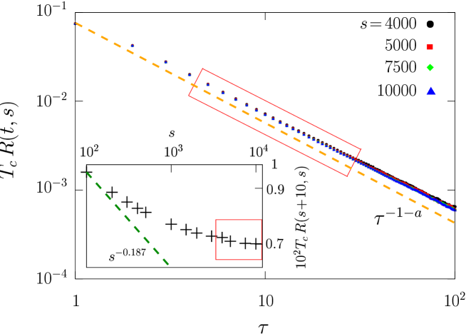
Figure 1: Autoresponse function $R(t,s)$ as a function of $\tau=t-s$ for different values of $s=4\cdot 10^{3},5\cdot 10^{3},7.5\cdot 10^{3}$, and $10^{4}$. The dashed line indicates the power-law behavior $R(t,s)\sim\tau^{-1-a}$ with $a=0.115$ (see Eq. (6)). The box indicates the points used to fit the value of the exponent $a_{\rm MC}$ (see the main text). In the inset $R(t,s)$ is plotted as a function of $s$ for fixed $\tau=10$. The dashed line indicates the behavior $\propto s^{-\Delta\alpha}$ predicted by LSI.1, with $\Delta\alpha$ given by Eq. (23). The box contains the points also present in the main figure.

The scaling behavior is expected to set in for $\tau,s\gg{\tau_{\rm micr}}$, i.e., the actual STSR is restricted to ${\tau_{\rm micr}}\ll\tau\ll s$. In the inset of Fig. 1 we report, for fixed $\tau=10\gg{\tau_{\rm micr}}\simeq 1$, the behavior of $T_{c}R(t,s)$ upon increasing $s$, eventually probing the STSR. In particular, according to LSI.1, one expects $R(s+10,s)\sim s^{-\Delta\alpha}$, whereas the actual data seemingly attain a plateau for $s\geq 3\cdot 10^{3}$ (highlighted by a box in the inset) setting an upper bound to the asymptotic value of $\Delta\alpha$: $\Delta\alpha<0.029(8)$, which definitely excludes the value (23) indicated in the inset as a dashed line. It seems therefore reasonable to conclude that $\Delta\alpha=0$ for large enough $s$. Note, however, that the behavior of $R(s+10,s)$ for $s\lesssim 10^{3}$ could be easily fitted by a power law with an effective exponent $\Delta\alpha_{\rm eff}\simeq 0.1$ which seemingly increases upon decreasing the largest value of $s$ included in the fit. If this observation carries over to the case of $\chi_{I}^{\rm(g)}(t,s)$ analyzed in Ref. HenkelLSI1 , it might explain the quite large $\Delta\alpha$ (23) which has been determined there on the basis of data with $s<200$. Repeating the previous analysis for different values of $\tau$ we conclude that for $s\geq 3\cdot 10^{3}$ (highlighted by a box in the inset) and $\tau<10^{2}$ (corresponding to $\tau/s\leq 0.032$), $R(\tau+s,s)$ is actually very close to its plateau value in the STSR, although small corrections of order $\tau/s$ are still present. The data corresponding to these selected range of $\tau$ and $s$, reported in the main plot in Fig. 1, display a quite good collapse onto a master curve $R(\tau+s,s)\sim\tau^{-1-a_{\rm MC}}$ with $a_{\rm MC}\simeq 0.095(2)$ when fitted in the region $5\leq\tau\leq 30$ (the corresponding points are highlighted by a box in the main plot of Fig. 1). This value is in reasonable agreement both with $a=0.115(2)$ and with $a-\Delta\alpha$, which are expected on the basis of Eqs. (3) and (9) and of LSI.1 with $\Delta\alpha<0.02$, respectively. In comparing these values one has to take into account that our Monte Carlo estimate $a_{\rm MC}\simeq 0.095(2)$ is seemingly affected by a systematic correction which reduces $a_{\rm MC}$ compared to its asymptotic value for $s\rightarrow\infty$.

Although the analysis of the scaling behavior of the response function in the STSR does not allow us to rule out the validity of LSI.1, at least it definitely indicates that $\Delta\alpha<0.02$.

A more effective comparison between the numerical data and the different theoretical predictions can be done by considering the quantity

$$g_{R}(t,s)\equiv\tau^{1+a}u^{-\theta}R(t,s),$$ (24)

for arbitrary $t>s$. According to the general scaling behavior Eq. (5), one expects

$$g_{R}(t,s)=A_{R}f_{R}(u),$$ (25)

i.e., $g_{R}(t,s)$ depends only on $u=t/s$ and is such that $\lim_{t\gg s}g_{R}(t,s)=A_{R}$. In addition, within the RG approach, $f_{R}(u)$ satisfies the condition (7), whereas within LSI.1 $f_{R}(u)$ is given by

$$f^{\rm(LSI.1)}_{R}(u)=u^{-\Delta\alpha}(u-1)^{\Delta\alpha},$$ (26)

(compare Eq. (15) with Eq. (5)) resulting in two different limiting behaviors for $u\rightarrow 1$:

$$\lim_{t\rightarrow s}g_{R}(t,s)=\begin{cases}B_{R},&\mbox{RG},\\ A_{R}(u-1)^{\Delta\alpha},&\mbox{LSI.1},\end{cases}$$ (27)

where $B_{R}=A_{R}f_{R}(1^{+})\neq 0$ (see after Eq. (9)). The qualitative difference between RG and LSI.1 in the STSR translates into the fact that for small values of the abscissa they predict the occurrence of a plateau and a power-law behavior with exponent $\Delta\alpha$, respectively, when $g_{R}(t,s)$ is plotted as a function of $u-1$. The log-log plot of $g_{R}(t,s)$ is presented in Fig. 2 for $s=10^{2}$, $2\cdot 10^{3}$, $7.5\cdot 10^{3}$, and $10^{4}$, which extend considerably the range of times investigated in Refs. HenkelLSI1 ; Pleim , with $s\leq 200$. We report only data with $\tau>2$ because, as discussed in Sec. I, scaling sets in only for $\tau\gg{\tau_{\rm micr}}\simeq 1$.

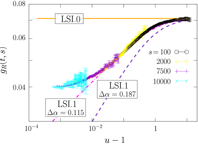
Figure 2: Scaling function $g_{R}(t,s)$ (see Eq. (24)) as a function of $u-1$ ($u=t/s>1$) for $s=100$, 2000, 7500, and 10000. The solid line is the prediction of LSI.0 whereas the dashed and dash-dotted lines are those of LSI.1 with $\Delta\alpha=0.187$ and $\Delta\alpha=0.115$, respectively. In all these cases the values $\theta=0.38$, $a=0.115$, and $A_{R}=0.07$ have been used.

For a fixed value of $s$, the statistical uncertainty affecting the data points in Fig. 2 increases upon increasing $u-1$, i.e., $t$, due to the fact that the value of the response function $R(t,s)\rightarrow 0$ becomes increasingly small and therefore comparable with statistical fluctuations. As a consequence of the typical scaling (4), this effect is expected to be more severe upon increasing $s$, as it is confirmed by comparing the data points with $s=10^{4}$ and $s=10^{2}$. The resulting data collapse in Fig. (2) is quite good (within the errorbars) and confirms that no significant corrections to scaling are present. From the behavior of $g_{R}(t,s)$ at large $u-1$ one determines the non-universal constant $A_{R}$:

$$A_{R}=0.071(2),$$ (28)

(obtained by fitting the data with $s=100$ and $u>7$) whereas in the opposite limit $u\rightarrow 1^{+}$ one finds (from the data with $s=7.5\cdot 10^{3},10^{4}$ and $u-1<1.2\cdot 10^{-3}$):

$$B_{R}=0.040(1),$$ (29)

and therefore one estimates

$$f_{R}(1^{+})=B_{R}/A_{R}=0.56(3).$$ (30)

III.1.1 Comparison with the available field-theoretical results

Note that $g_{R}(t,s)/A_{R}=f_{R}(u)$ characterizes the universal scaling behavior of the response function within the Ising universality class with purely dissipative dynamics. In turn, this fact can be used in order to determine the associated scaling function in simplified models, e.g., field-theoretical (FT) ones FT-Is ; Cala2 ; cg-rev belonging to this universality class. In particular, in Ref. FT-Is the scaling function for the spatial Fourier transform of $R_{r}(t,s)$ (Eq. (1)) was determined up to the first order in $\epsilon=4-d>0$ where $d$ is the spatial dimensionality of the model. This result allows the calculation of $f_{R}(u)$ (see Eqs. (5) and (24)), yielding

$$f^{\rm(FT)}_{R}(u)=1+O(\epsilon^{2}),$$ (31)

which actually does not reproduce the non-trivial behavior observed in Fig. 2 and the actual value of $f_{R}(1^{+})$ determined numerically (see Eq. (30)). On the other hand, as in the case of the scaling function of $\sum_{\bf r}R_{r}(t,s)$ studied analytically in Ref. Cala2 , one expects non-trivial corrections to $f_{R}^{\rm(FT)}(u)$ at $O(\epsilon^{2})$ which might reproduce at least the qualitative features of the numerical data (such as the fact that $g_{R}(t,s)\leq A_{R}$). The calculation of such corrections, however, is beyond the scope of the present study.

III.1.2 Comparison with LSI

The mastercurve in Fig. 2 clearly exhibits a plateau at small $u-1$ which excludes the power-law behavior predicted in this regime by LSI.1 (or, at least, it reduces significantly the upper bound to $\Delta\alpha$ which results from Fig. 1 nota2 ). This conclusion is also confirmed by comparing the numerical data for $g_{R}(t,s)$ with the prediction (25), where $f_{R}(u)$ is given by Eq. (26) and $A_{R}$ by the fitted value (28). In Fig. 2 we present this comparison for $\Delta\alpha=0$ (solid line), corresponding to LSI.0, $\Delta\alpha=0.187$ (dashed line), corresponding to the estimate (23) of Ref. HenkelLSI1 , and $\Delta\alpha=0.115$ (dash-dotted line) — which we have determined from the best fit to the actual data. Clearly, both LSI.0 and LSI.1 with the value of $\Delta\alpha$ determined in Ref. HenkelLSI1 do not capture correctly the scaling behavior of the response function already for $u\simeq 6$ and in particular they overestimate and underestimate the numerical $g_{R}(t,s)$, respectively. The choice $\Delta\alpha=0.115$, however, results in a good fit of the numerical data down to $u-1\simeq 2\cdot 10^{-2}$. In spite of that, sizable discrepancies are anyhow observed for smaller values of $u-1$ (STSR) and no further improvement is actually possible by varying $\Delta\alpha$. In passing we mention that a similar situation is also encountered when comparing the predictions of LSI.1 with the scaling behavior of the aging response function within the directed percolation universality class Gamba ; Hinrich .

The conclusion we can draw so far is that the scaling behavior of the impulse response function $R(t,s)$ does not agree with the prediction of LSI.1 even though the latter actually provides a good fit to the numerical data for $t/s-1\gtrsim 2\cdot 10^{-2}$.

III.2 Integrated local response functions

In this Subsection we discuss the behavior of the local integrated response function (see Eq. (17)), which is given by $\chi_{I}^{\rm(l)}(t,s)=\chi(t,[s/2,s])$ in terms of the quantity (18) measured in the simulations. This integrated response function has also been considered in Refs. noiTRM ; noiRd2 .

According to the general scaling behavior of $R(t,s)$ (see Eq. (5)), one expects

$$\chi_{I}^{\rm(l)}(t,s)=A_{R}s^{-a}u^{\theta-1}(u-1)^{-a}f_{\chi,{\rm l}}(u)$$ (32)

where the universal scaling function $f_{\chi}^{\rm(l)}(u)$ is given, in terms of the scaling function $f_{R}$, by

$$f_{\chi,{\rm l}}(u)=(1-u^{-1})^{a}\int_{1/2}^{1}\!\!{\rm d}x\,x^{-\theta}\left(1-\frac{x}{u}\right)^{-1-a}f_{R}(u/x)\;,$$ (33)

and is such that $f_{\chi,{\rm l}}(u\gg 1)=\kappa_{\theta}$ with $\kappa_{\theta}=(1-2^{-1+\theta})/(1-\theta)$ ($\kappa_{\theta}\simeq 0.564$ in two dimensions). In particular, the prediction of LSI.1 is obtained from $f_{R}^{\rm(LSI.1)}(u)$ given in Eq. (26):

$$f^{\rm(LSI.1)}_{\chi,{\rm l}}(u)=\frac{(1-u^{-1})^{a}}{1-\theta}\left[{}_{2}F_{1}(1-\theta,1+a-\Delta\alpha,1/u)-2^{\theta-1}{}_{2}F_{1}(1-\theta,1+a-\Delta\alpha,1/(2u))\right],$$ (34)

where ${}_{2}F_{1}$ is the hypergeometric function and the case of LSI.0 is recovered for $\Delta\alpha=0$. In order to compare the different theoretical predictions we consider the function

$$g_{\chi,{\rm l}}(t,s)\equiv\tau^{a}u^{1-\theta}\chi_{I}^{\rm(l)}(t,s)$$ (35)

which, according to Eq. (32), is a function of $u=t/s$

$$g_{\chi,{\rm l}}(t,s)=A_{R}f_{\chi,{\rm l}}(u)$$ (36)

such that $A_{\chi,{\rm l}}\equiv\lim_{t\gg s}g_{\chi,{\rm l}}(t,s)=A_{R}\kappa_{\theta}$. In the opposite limit, instead,

$$\lim_{t\rightarrow s}g_{\chi,{\rm l}}(t,s)=\begin{cases}B_{\chi,{\rm l}}=B_{R}/a,&\mbox{RG},\\ A_{R}(u-1)^{\Delta\alpha}/(a-\Delta\alpha),&\mbox{LSI.1},\end{cases}$$ (37)

which is valid under the assumption $a,a-\Delta\alpha>0$ and which reflects the different behaviors of $f_{R}(u\rightarrow 1^{+})$ within RG and LSI.1 (see Eqs. (7) and (26), respectively). In Fig. 3 we plot $g_{\chi,{\rm l}}(t,s)$ for different values of $s$, which are slightly larger than those considered in Ref. Pleim ; HenkelLSI1 but smaller than the larger values which Fig. 2 refers to.

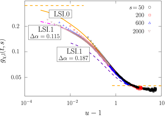
Figure 3: Scaling function $g_{\chi,{\rm l}}(t,s)$ (see Eq. (35)) as a function of $u-1$ ($u=t/s>1$) for $s=50$, 200, 600, and 2000. The solid line is the prediction of LSI.0 whereas the dashed and dash-dotted lines are those of LSI.1 with $\Delta\alpha=0.187$ and $\Delta\alpha=0.115$, respectively. In all these cases the values $\theta=0.38$, $a=0.115$, and $A_{R}=0.07$ have been used. The horizontal dashed line on the left (right) indicates the limiting value $B_{R}/a$ ($A_{R}\kappa_{\theta})$ expected for $u\to 1$ ($u\to\infty$) according to the RG and scaling behavior (see Eq. (37)) where $A_{R}$ and $B_{R}$ have been determined from the behavior of $g_{R}(t,s)$ (see Eqs. (28) and (29)).

For $s\geq 600$ and $u-1\gtrsim 10^{-2}$ one observes a rather good collapse onto a single master curve which depends only on $u$, in agreement with the scaling (32). At smaller values of $u-1$ the actual scaling behavior is accessed only for increasingly larger values of $s$ such that $\tau=t-s>{\tau_{\rm micr}}$, i.e., for $s>{\tau_{\rm micr}}/(u-1)$. From the large-$u$ behavior of $g_{\chi,{\rm l}}(t,s)$ we determine the non-universal constant

$$A_{\chi,{\rm l}}=0.036(3)$$ (38)

in marginal agreement with the expected value $A_{R}\kappa_{\theta}=0.040(1)$ resulting from the estimate of $A_{R}$ given in Eq. (28). Note that while $g_{R}(t,s)\leq A_{R}$, here we find $g_{\chi,{\rm l}}(t,s)\geq A_{\chi,{\rm l}}$.

III.2.1 Comparison with the available field-theoretical results:

The universal scaling behavior of $\chi_{I}^{\rm(l)}(t,s)$ within the Ising universality class with purely dissipative dynamics is characterized by $g_{\chi,{\rm l}}(t,s)/A_{\chi,{\rm l}}=f_{\chi,{\rm l}}(u)$ which can also be studied within field-theoretical models FT-Is ; Cala2 ; cg-rev . As a consequence of the fact that $f^{\rm(FT)}_{R}(u)=1+O(\epsilon^{2})=f_{R}^{\rm(LSI.0)}(u)+O(\epsilon^{2})$ (see Eq. (31) and Eq. (26) with $\Delta\alpha=0$), one finds, from Eq. (33), $f^{\rm(FT)}_{\chi,{\rm l}}(u)=f_{\chi,{\rm l}}^{\rm(LSI.0)}(u)+O(\epsilon^{2})$, where $f_{\chi,{\rm l}}^{\rm(LSI.0)}(u)$ is given by Eq. (34) with $\Delta\alpha=0$. The resulting prediction $A_{R}f^{\rm(FT)}_{\chi,{\rm l}}(u)$ for $g_{\chi,{\rm l}}(t,s)$ is shown in Fig. 3 as LSI.0: The differences with the numerical data are less severe than in the case of $A_{R}f_{R}^{\rm(FT)}(u)$ for $g_{R}(t,s)$ in Fig. 2. In particular, for $u\rightarrow 1^{+}$ one has $f^{\rm(FT)}_{\chi,{\rm l}}(1^{+})=f_{\chi,{\rm l}}^{\rm(LSI.0)}(1^{+})+O(\epsilon^{2})=1/a+O(\epsilon^{2})$ (see Eq. (34) with $\Delta\alpha=0$ and $u\rightarrow 1^{+}$) footnote , yielding the plateau in the FT prediction reported in Fig. 3 as a dashed line, which overestimates the actual numerical value. It would be interesting to see whether the corrections of $O(\epsilon^{2})$ to $f^{\rm(FT)}_{\chi,{\rm l}}(u)$ account for such a difference.

III.2.2 Comparison with LSI:

As in the case of the impulse response function, the different qualitative behavior of the LSI.1 and RG predictions should be displayed for $u-1\rightarrow 0$ according to Eq. (37), but the data presented in Fig. 3 are not actually able to detect such a difference. However, the trend of the data is compatible with the RG prediction $\lim_{t\rightarrow s}g_{\chi,{\rm l}}(t,s)=B_{R}/a\simeq 0.35$ (see Eq. (29)). For comparison we plot also Eq. (36) with $f_{\chi,{\rm l}}^{\rm(LSI.1)}$ predicted by LSI (see Eq. (34)), $A_{R}=0.063$ (note that this is slightly smaller than the previous estimate Eq. (28)) and for the different values of $\Delta\alpha$ already considered in Fig. 2: $\Delta\alpha=0$ (solid line), corresponding to LSI.0, $\Delta\alpha=0.187$ (dashed line), corresponding to the estimate (23) of Ref. HenkelLSI1 , and $\Delta\alpha=0.115$ (dash-dotted line). As in the case of $R(t,s)$, both LSI.0 and LSI.1 with $\Delta\alpha=0.187$ do not provide a good approximation of the actual data already for $u-1\lesssim 0.1$ and $1$, respectively, whereas LSI.1 with $\Delta\alpha=0.115$ shows visible discrepancies only for $u-1\lesssim 4\cdot 10^{-3}$, when compared to the curve with $s=2000$, which is expected to display smaller corrections to scaling. The result of the integration over time has been to reduce by almost one order of magnitude the value of $u-1$ below which LSI.1 with $\Delta\alpha=0.115$ does not agree with the numerical data in the scaling regime (from $\simeq 2\cdot 10^{-2}$ for $R(t,s)$ to $\simeq 2\cdot 10^{-3}$ for $\chi_{I}^{\rm(l)}(t,s)$). By looking solely at Fig. 3 one would naturally conclude that the scaling behavior of $\chi_{I}^{\rm(l)}(t,s)$ is actually described by LSI.1 with $\Delta\alpha=0.115$: The corrections for $u-1\lesssim 4\cdot 10^{-3}$ seemingly vanish upon increasing $s$.

III.3 Integrated global response functions

We finally consider the global intermediate response function $\chi_{I}^{\rm(g)}(t,s)$ (see Eqs. (14)) which was introduced and studied in Ref. Pleim in order to highlight discrepancies between the numerical data and the prediction of LSI.0 in the case of the the two- and three-dimensional Ising model with Glauber dynamics. The same data presented in Ref. Pleim have later on been found in agreement with the prediction of LSI.1 HenkelLSI1 . In terms of the quantity (19) measured in the simulations, $\chi_{I}^{\rm(g)}(t,s)$ is given by $\chi_{I}^{\rm(g)}(t,s)=\hat{\chi}_{k=0}(t,[s/2,s])$ and it is therefore a space integrated, or global, quantity. In fact, $\sum_{\bf r}R_{r}(t,t^{\prime})$ is the response function of the total magnetization.

In this Subsection we focus on the comparison between $\chi_{I}^{\rm(g)}(t,s)$ and LSI, being the one with the corresponding field-theoretical predictions Cala2 already discussed in Ref. Pleim .

According to general scaling arguments (see, e.g., Ref. Pleim ; cg-rev ), the global response function $\hat{R}_{k=0}(t,s)$ is expected to scale as

$$\hat{R}_{k=0}(t,s)={\mathcal{A}}_{R}s^{-1-a+d/z}u^{\theta}(u-1)^{-1-a+d/z}{\mathcal{F}}_{R}(u),$$ (39)

where the non-universal constant ${\mathcal{A}}_{R}$ is fixed by the condition ${\mathcal{F}}_{R}(u\gg 1)=1$, and the function ${\mathcal{F}}_{R}(u)$ is universal. Within the RG approach one additionally finds that ${\mathcal{F}}_{R}(1^{+})\neq 0$ and finite, in analogy to Eq. (7). As a result of the factorization (13) of the space dependence of $R_{r}(t,s)$, the scaling behavior of the Fourier transform $\hat{R}_{k=0}(t,s)=\int\!{\rm d}{\bf r}R_{r}(t,s)$ is given by Eq. (39) with

$${\mathcal{F}}^{\rm(LSI.1)}_{R}(u)=u^{-\Delta\alpha}(u-1)^{\Delta\alpha},$$ (40)

i.e., it has the same expression as in the case of $R(t,s)$ but with the formal substitutions $A_{R}\mapsto{\mathcal{A}}_{R}=A_{R}\int\!{\rm d}{\bf x}\Phi({\bf x})$ and $a\mapsto a-d/z$. Note that, as in the case of the local response function, LSI.1 and scaling arguments predicts two qualitatively different behaviors of ${\mathcal{F}}_{R}(u\rightarrow 1^{+})$. The scaling form of $\chi_{I}^{\rm(g)}(t,s)$ is easily calculated on the basis of Eq. (39), yielding

$$\chi_{I}^{\rm(g)}(t,s)={\mathcal{A}}_{R}t^{-a+d/z}u^{\theta-1}f_{\chi,{\rm g}}(u)$$ (41)

where

$$f_{\chi,{\rm g}}(u)=\int_{1/2}^{1}\!\!{\rm d}x\,x^{-\theta}\left(1-\frac{x}{u}\right)^{-1-a+d/z}{\mathcal{F}}_{R}(u/x),$$ (42)

such that $f_{\chi,{\rm g}}(u\gg 1)=\kappa_{\theta}$. In particular the prediction of LSI.1 is readily found as (see Eqs. (33) and (34))

$$f_{\chi,{\rm g}}^{\rm(LSI.1)}(u)=\int_{1/2}^{1}\!\!{\rm d}x\,x^{-\theta}\left(1-\frac{x}{u}\right)^{-1-a+d/z+\Delta\alpha}=\left[(1-u^{-1})^{-a}f_{\chi,{\rm l}}^{\rm(LSI.1)}(u)\right]_{a\mapsto a-d/z}\;.$$ (43)

As in the previous cases, in order to compare the numerical data with the prediction of LSI.1 we consider the quantity

$$g_{\chi,{\rm g}}(t,s)\equiv t^{a-d/z}u^{1-\theta}\chi_{I}^{\rm(g)}(t,s)$$ (44)

which, according to Eq. (41) is a function of $u=t/s$:

$$g_{\chi,{\rm g}}(t,s)={\mathcal{A}}_{R}f_{\chi,{\rm g}}(u)$$ (45)

such that ${\mathcal{A}}_{\chi,{\rm g}}\equiv\lim_{t\gg s}g_{\chi,{\rm g}}(t,s)={\mathcal{A}}_{R}\kappa_{\theta}$. Differently from the previous cases, the behavior of $g_{\chi,{\rm g}}(t,s)$ for $t\rightarrow s$ is predicted to be qualitatively the same both by scaling arguments and LSI.1: The integral in Eq. (42) is finite for $u\rightarrow 1$, whatever the actual behavior of ${\mathcal{F}}_{R}(x/u\rightarrow 1^{+})$ is, as long as ${\mathcal{F}}_{R}(u\rightarrow 1^{+})\sim(u-1)^{\sigma}$ with $\sigma>a-d/z$, which is the case here. In Fig. 4 we plot $g_{\chi,{\rm g}}(t,s)$ for different values of $s$, which are comparable to those considered in Ref. Pleim ; HenkelLSI1 but generally smaller than the values which Figs. 2 and 3 refer to.

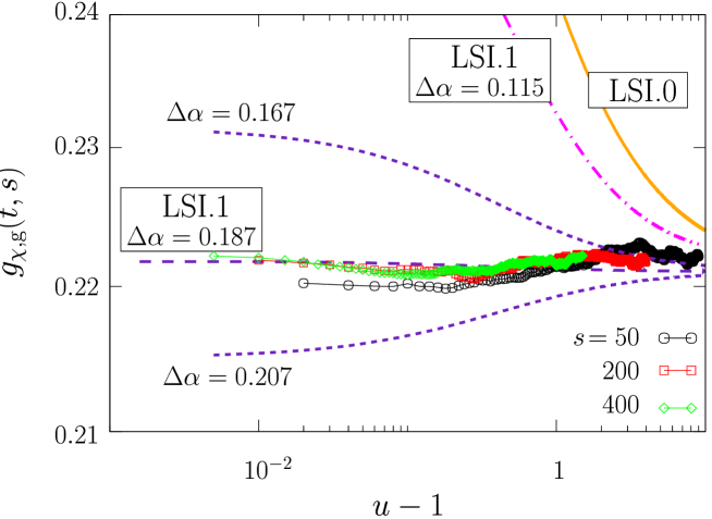
Figure 4: Scaling function $g_{\chi,{\rm g}}(t,s)$ (see Eq. (44)) as a function of $u-1$ ($u=t/s>1$) for $s=50$, 200, and 400. The solid line is the prediction of LSI.0 whereas the dashed and dash-dotted lines are those of LSI.1 with $\Delta\alpha=0.187$ and $\Delta\alpha=0.115$, respectively. The two additional dashed lines represent the upper and lower bound to $\Delta\alpha$ provided in Ref. HenkelLSI1 and resulting from the fit of $\chi_{I}^{\rm(g)}(t,s)$ with the prediction of LSI.1. In all these cases $\theta=0.38$, $a=0.115$, and ${\mathcal{A}}_{R}=0.3895$ have been used.

The data sets corresponding to $s=200$ and 400 collapse to a reasonable extent, whereas the set corresponding to $s=50$ still departs from the previous two because of corrections to the scaling behavior. For larger values of $u-1$, instead, statistical errors increase due to a poor statistics. However, our point here is not to determine the scaling function with high accuracy, but compare its features to those of the prediction of LSI.1. As it was already clear from the numerical results presented in Fig. 2(a) of Ref. Pleim (which Fig. 4 has to be compared to footnote2 ), $g_{\chi,{\rm g}}(t,s)$ does not vary too much as a function of $u$, being almost flat for $0.3\lesssim u-1\lesssim 10$ while slightly increasing upon decreasing $u-1<0.3$ (about 2% in the interval $0.05\lesssim u-1\lesssim 0.3$) and decreasing upon increasing $u-1>10$ (by less than 2%). Analogous behavior has been observed in the three-dimensional Ising model (see Fig. 2(b) in Ref. Pleim ). From the large-$u$ behavior of $g_{\chi,{\rm g}}(t,s)$ we estimate the non-universal constant

$${\mathcal{A}}_{\chi,{\rm g}}=0.221(1).$$ (46)

(Which has actually been obtained on the basis of the data with $s=200$ and $u\gtrsim 3$.) In Fig. 4 we also plot ${\mathcal{A}}_{R}f_{\chi,{\rm g}}^{\rm(LSI.1)}(u)$ where $f_{\chi,{\rm g}}^{\rm(LSI.1)}(u)$ in given by Eq. (42) and ${\mathcal{A}}_{R}={\mathcal{A}}_{\chi,{\rm g}}/\kappa_{\theta}$ has been fixed to $0.3895$. In particular we report the predictions for $\Delta\alpha=0$ (solid line), $\Delta\alpha=0.115$ (dash-dotted line) and $\Delta\alpha=0.187(20)$ (dashed and dotted lines). The prediction of LSI.1 with $\Delta\alpha=0.187$ provides a quite good fit of the actual scaling behavior, in complete agreement with what found in Ref. HenkelLSI1 , where this value of $\Delta\alpha$ was determined as the best-fit parameter. By looking at the integral in the expression of $f^{\rm(LSI.1)}_{\chi,{\rm g}}(u)$ (see Eq. (43)) it becomes clear why $f^{\rm(LSI.1)}_{\chi,{\rm g}}(u)$ is so accurate in reproducing the almost constant behavior of the numerical data for $g_{\chi,{\rm g}}(u)$ as a function of $u$: For $\Delta\alpha=\Delta\alpha_{0}\equiv 1+a-d/z$, $f^{\rm(LSI.1)}_{\chi,{\rm g}}(u)$ becomes constant. In two dimensions one finds $\Delta\alpha_{0}=0.192(2)$ which is within the interval determined in Ref. HenkelLSI1 . On the other hand, both the prediction of LSI.1 with $\Delta\alpha=0.115$ — which was providing the best fit to $R(t,s)$ — and of LSI.0 are quite far from the actual numerical data. In particular, the fact that LSI.1 with $\Delta\alpha=0.115$ well describes both $R(t,s)$ and $\chi_{I}^{\rm(l)}(t,s)$ but not $\chi_{I}^{\rm(g)}(t,s)$ suggests that the factorization of the space dependence (13) might not be a good approximation of the actual scaling behavior.

On the basis of Figs. 2, 3, and 4 we can conclude that possible integrations of local quantities over time and over space strongly affect the agreement between numerical data and the corresponding prediction of LSI.1. Accordingly, the exponent $\Delta\alpha$ which characterizes such a prediction can not be regarded as an additional model-dependent exponents but simply as a fitting parameter the optimal value of which depends on the specific quantity considered. Indeed, LSI.1 with $\Delta\alpha=0.187(20)$ describes correctly the behavior of $\chi_{I}^{\rm(g)}(t,s)$ but it fails in the case of the related $R(t,s)$. Conversely, LSI.1 with $\Delta\alpha=0.115$ describes very well, for $t/s-1>10^{-2}$, the behavior of both $R(t,s)$ and $\chi_{I}^{\rm(l)}(t,s)$ but it fails in the case of the global response function $\chi_{I}^{\rm(g)}(t,s)$.

IV Quenches to $T_{\rm f}<T_{c}$

In Sec. I we have pointed out that the prediction (16) of LSI.1 with $\Delta\alpha\neq 0$ does not become stationary in the STSR, in contrast to what the response function actually does. Even arguing that the validity of LSI.1 might be restricted only to the aging regime does not help for quenches at the critical point: The multiplicative structure in Eqs. (8) and (10) — a direct consequence of scale invariance — leaves no room for LSI.1 to describe $R^{\rm(ag)}$ without spoiling the quasi-equilibrium behavior of $R(t,s)$ in the STSR. For $T_{\rm f}<T_{c}$, however, the crossover between $R^{\rm(eq)}(\tau;T_{\rm f})$ and $R^{\rm(ag)}(t,s)$ does not occur multiplicatively but additively, as we shall discuss shortly. Then, the criticism moved to LSI.1 for critical quenches does not extend to below $T_{c}$.

Indeed, in quenches below $T_{c}$, two-time quantities such as the autoresponse function naturally split as Bouchaud97 ; Cugliandolo ; noiTeff

$$R(t,s)=R^{\rm(eq)}(\tau;T_{\rm f})+R^{\rm(ag)}(t,s).$$ (47)

This additive structure is a direct consequence of the phenomenology of phase-ordering Bray , where a patchwork of compact growing domains, internally in equilibrium, evolve through defect displacement and/or annihilation. Fast equilibrium fluctuations inside domains are responsible for $R^{\rm(eq)}(\tau;T_{\rm f})$, whereas the slow degrees of freedom associated to the dynamics of defects give rise to $R^{\rm(ag)}(t,s)$. One easily verifies that Eq. (47) renders Eq. (3) in the STSR when $R^{\rm(ag)}$ is given by Eqs. (5) and (11) (i.e., by LSI.1): In this sector, in fact, $u=1+\tau/s\to 1$ and therefore $R^{\rm(ag)}(t,s)\sim s^{-\Delta\alpha}\tau^{-1-a+\Delta\alpha}$ which, if $\Delta\alpha>0$, becomes negligible for $s\to\infty$ in comparison to $R^{\rm(eq)}(\tau;T_{\rm f})$. In the aging regime, instead, the opposite is true: $R^{\rm(eq)}(\tau;T_{\rm f})$ for $u>1$ becomes negligible compared to $R^{\rm(ag)}(t,s)$. In scalar systems, which we are interested in here, this is due to the fast (exponential) decay of $R^{\rm(eq)}(\tau;T_{\rm f})$ over a timescale $\tau_{eq}(T_{\rm f})\sim\xi^{z_{g}}(T_{\rm f})$, where $\xi(T_{\rm f})$ is the correlation length of the equilibrium state at $T=T_{\rm f}$ with broken symmetry. In the aging regime one eventually has $\tau\gg\tau_{eq}(T_{\rm f})$ and hence $R^{\rm(eq)}(\tau;T_{\rm f})$ becomes (exponentially) small compared to $R^{\rm(ag)}(t,s)$ for $u>1$, yielding $R(t,s)=R^{\rm(ag)}(t,s)$, i.e., the response function is very well approximated by $R^{\rm(ag)}(t,s)$.

Now, as stated in the Introduction, in the analytically solved instances of phase ordering such as the $d=1$ Ising model Lippiello ; God1 quenched to $T_{\rm f}=0$ footnote1d and the time-dependent Ginzburg-Landau model within the Gaussian auxiliary field approximation berthier ; EPJ ; Mazenko , Eq. (11) holds footnoteclass . This result has also been verified with high accuracy via numerical simulation of the Ising model in $2,3$ and $4$ dimensions with Glauber dynamics noiTRM ; noiRd2 , where $z_{g}=2$, and of the one-dimensional Ising model with Kawasaki dynamics noialg , where $z_{g}=3$. Therefore, in the case of subcritical quenches the form of $R^{\rm(ag)}$ predicted by LSI.1 would fit in the analytical and numerical results with

$$\Delta\alpha=1/z_{g}.$$ (48)

It must be stressed that contrary to the case of critical quenches, $\Delta\alpha\neq 0$ is not in conflict with the time translational invariant behavior of the response function at short times because of the additive structure of Eq. (47). Note, however, that numerical results for $\chi(t,[0,s])$ and $\hat{\chi}_{k=0}(t,[0,s])$ in the two- and three-dimensional Ising model with Glauber dynamics MHenkel , quenched to $T_{\rm f}<T_{c}$, are seemingly consistent with $\Delta\alpha=0$ (see Ref. H-wdb for more details). This conclusion might be biased by the fact that these quantities, at variance with $R(t,s)$ studied in Ref. noiRd2 , are affected by quite large corrections to scaling noiTRM .

V Summary and conclusions

We have studied in detail, via Monte Carlo simulations, the impulse autoresponse function $R(t,s)$ [see Eqs. (1) and (2)] and the associated (intermediate) integrated local and global response functions $\chi_{I}^{\rm(l)}(t,s)$ [Eq. (17)] and $\chi_{I}^{\rm(g)}(t,s)$ [Eq. (14)], respectively, of the two-dimensional Ising model with Glauber dynamics, after a quench from high temperature to the critical point.

We highlighted the universal non-equilibrium scaling behaviors of these quantities and we compared them with the predictions derived from the theory of Local Scale Invariance in its two recently proposed versions, referred to as LSI.0 [Eqs. (12) and (13)] and LSI.1 [Eqs. (15) and (13)]. The scaling form of $R(t,s)$ predicted by LSI.1 depends on the additional parameter $\Delta\alpha$, compared to the prediction of LSI.0, which is actually recovered for $\Delta\alpha=0$ (see Sec. I). On the basis of our numerical analysis we conclude that:

• $T_{c}R(t,s)$ becomes — as generally expected — time-translational invariant in the short-time separation regime which is accessed by increasing $s\gg{\tau_{\rm micr}}$ while keeping fixed $\tau=t-s$ (see Fig. 1). This behavior is consistent with the prediction of LSI.0 but not with the one of LSI.1 (with $\Delta\alpha\neq 0$, see Eq. (15)).

• The scaling behavior of $R(t,s)$ (see Fig. 2 and Eq. (24)) is correctly captured neither by LSI.0 nor by LSI.1. However, LSI.1 with $\Delta\alpha=0.115$ yields a good fit of the actual data only for $t/s-1>2\cdot 10^{-2}$. Figure 2 — properly normalized by $A_{R}$ (see Eq. (28)) — provides a very accurate numerical determination of the universal scaling function of $R(t,s)$ in a wider range of times compared to previous numerical studies.

• Apparently, the scaling behavior of $\chi_{I}^{\rm(l)}(t,s)$ (see Fig. 3 and Eq. (35)) is correctly captured by LSI.1 with $\Delta\alpha=0.115$. The small discrepancies which are visible for $t/s-1<4\cdot 10^{-3}$ can be due either to non-universal correction to scaling (in which case they should disappear upon increasing $s$) or to the fact that the actual scaling function of $\chi_{I}^{\rm(l)}(t,s)$ deviates from LSI.1 at smaller values of $t/s-1$ (as in the case of $R(t,s)$). The data at our disposal do not allow one to discriminate between these two options.

• In agreement with previous studies Pleim , we find that the scaling behavior of $\chi_{I}^{\rm(g)}(t,s)$ (see Fig. 4 and Eq. (44)) is encoded in a scaling function $g_{\chi,{\rm g}}(t,s)$ which varies less than 4% in a wide range of times. Although the quality of the data presented in Fig. 4 does not allow an accurate determination of the scaling function, it is sufficient in order to conclude that both LSI.0 and LSI.1 with $\Delta\alpha=0.115$ have no chance to describe it correctly, whereas — as noted in Ref. HenkelLSI1 — LSI.1 with $\Delta\alpha=0.187(20)$ actually provides a better approximation.

The evidences summarized above lead to the conclusion that the scaling forms predicted analytically by LSI.1 for the various quantities related to $R_{r}(t,s)$ provide, in some cases, accurate fitting forms but cannot be considered to be exact, at least for quenches at the critical point. It would be interesting to compare our numerical determination of the universal scaling function of $R(t,s)$ (see Fig. 2) with the predictions of different analytical approaches such as, e.g., field-theoretical ones.

References

- (1) L. F. Cugliandolo, Lecture notes in Slow Relaxation and Non Equilibrium Dynamics in Condensed Matter, Les Houches Session 77 July 2002, edited by J. -L. Barrat, J. Dalibard, J. Kurchan and M. V. Feigel’man (Springer, 2003) [e-print cond-mat/0210312].
- (2) C. Godrèche and J. M. Luck, J. Phys.: Condens. Matter 14, 1589 (2002).
- (3) P. Calabrese and A. Gambassi, J. Phys. A: Math. Gen. 38, R133 (2005).
- (4) C. Godrèche and J. M. Luck, J. Phys. A: Math. Gen. 33, 9141 (2000).
- (5) H. K. Janssen, B. Schaub, and B. Schmittmann, Z. Phys. B 73 539 (1989); H. K. Janssen, On the renormalized field theory of nonlinear critical relaxation, in From Phase Transitions to Chaos– Topics in Modern Statistical Physics, edited by G. Györgyi, I. Kondor, L. Sasvári, T. Tel (World Scientific, Singapore, 1992).
- (6) Equation (5) is expected to capture the universal scaling behavior of the response function which, in lattice models, sets in only for . Accordingly, the notation in Eq. (7) emphasize the fact that the limit of has to be taken in such a way to satisfy this condition, i.e., with fixed .
- (7) F. Corberi, E. Lippiello, and M. Zannetti, Phys. Rev. E 68, 046131 (2003).
- (8) F. Corberi, E. Lippiello, and M. Zannetti, Phys. Rev. E 72, 056103 (2005).
- (9) E. Lippiello, F. Corberi, and M. Zannetti, Phys. Rev. E 74, 041113 (2006).
- (10) E. Lippiello and M. Zannetti, Phys. Rev. E 61, 3369 (2000).
- (11) C. Godrèche and J. M. Luck, J. Phys. A: Math. Gen. 33, 1151 (2000).
- (12) The one-dimensional Ising model quenched to dispalys a breaking of ergodicity and therefore its behavior is expected to be more akin to the one observed during phase ordering than to the critical one.
- (13) L. Berthier, J. L. Barrat, and J. Kurchan, Eur. Phys. J. B 11, 635 (1999).
- (14) F. Corberi, E. Lippiello, and M. Zannetti, Eur. Phys. J. B 24, 359 (2001).
- (15) G. F. Mazenko, Phys. Rev. E 69, 016114 (2004).
- (16) F. Corberi, C. Castellano, E. Lippiello, and M. Zannetti, Phys. Rev. E 70, 017103 (2004).
- (17) M. Henkel and M. Pleimling, Phys. Rev. E 68, 065101(R) (2003).
- (18) E. Lorenz and W. Janke, Europhys. Lett. 77, 10003 (2007).
- (19) A. J. Bray, Adv. Phys. 43, 357 (1994).
- (20) M. Henkel, M. Pleimling, C. Godrèche, and J. M. Luck, Phys. Rev. Lett. 87, 265701 (2001).
- (21) M. Henkel and F. Baumann, J. Stat. Mech.: Theor. Exp. P07015 (2007).
- (22) M. Henkel, Nucl. Phys. B 641, 405 (2002); A. Picone and M. Henkel, Nucl. Phys. B 688, 217 (2004).
- (23) M. Henkel, T. Enss, and M. Pleimling, J. Phys. A: Math. Gen. 39, L589 (2006).
- (24) F. Baumann, S. Stoimenov, and M. Henkel, J. Phys. A: Math. Gen. 39, 4095 (2006).
- (25) T. Enss, M. Henkel, A. Picone, and U. Schollwöck, J. Phys. A: Math. Gen. 37, 10479 (2004).
- (26) G. Odor, J. Stat. Mech.: Theor. Exp. L11002 (2006).
- (27) M. Henkel, J. Phys. Condens. Matter 19, 065101 (2007).
- (28) M. Henkel and M. Pleimling, Europhys. Lett. 76, 561 (2006).
- (29) M. Pleimling and A. Gambassi, Phys. Rev. B 71, 180401(R) (2005).
- (30) H. Hinrichsen, J. Stat. Mech.: Theor. Exp. L06001 (2006).
- (31) F. Baumann and A. Gambassi, J. Stat. Mech.: Theor. Exp. P01002 (2007).
- (32) F. Corberi, E. Lippiello, and M. Zannetti, Phys. Rev. E 65, 046136 (2002).
- (33) S. Abriet and D. Karewski, Eur. Phys. J. B 37, 47 (2004); ibid. 41, 79 (2004).
- (34) P. Calabrese and A. Gambassi, Phys. Rev. E 66, 066101 (2002).
- (35) M. Henkel and M. Pleimling, J. Phys. Cond. Matt. 17, S1899 (2005).
- (36) P. Mayer and P. Sollich, J. Phys. A: Math. Theor. 40, 5823 (2007).
- (37) E. Lippiello, F. Corberi, and M. Zannetti, Phys. Rev. E 71, 036104 (2005).
- (38) R. J. Glauber, J. Math. Phys. 4, 294 (1963).
- (39) C. Chatelain, J. Phys. A: Math. Gen. 36, 10739 (2003).
- (40) M. P. Nightingale and W. W. Blöte, Phys. Rev. B 62, 1089 (2000).
- (41) P. Grassberger Physica A, 214, 547 (1995); see also erratum ibid. 217, 227 (1995).
- (42) P. Calabrese and A. Gambassi, Phys. Rev. E 65, 066120 (2002); Acta Phys. Slov. 52, 311 (2002); For a pedagogical introduction, see: A. Gambassi, J. Phys.: Conf. Series 40, 13 (2006).
- (43) Fitting the points in the region with one finds depending on the value of which corresponds to the selected points.
- (44) Within FT, and therefore up to would be logarithmically divergent for . On the other hand, one can improve the estimate of by using in Eq. (34) the actual values of the exponents in two dimensions.
- (45) The raw data for corresponding to Fig. 4 do actually reproduce those presented in Ref. Pleim ; HenkelLSI1 after a multiplication by a normalization factor .
- (46) J. P. Bouchaud, L. F. Cugliandolo, J. Kurchan, and M. Mézard in Spin Glasses and Random Fields edited by A.P.Young (World Scientific, Singapore, 1997).
- (47) F. Corberi, E. Lippiello, and M. Zannetti, J. Stat. Mech.: Theor. Exp. P12007 (2004).
- (48) Note that in Tab. 2 of Ref. H-wdb these models are questionably listed among those undergoing critical coarsening.