Spitzer Observations of the ii Region NGC 2467: An Analysis of Triggered Star Formation11affiliation: Based on observations with the Spitzer Space Telescope
Abstract
We present new Spitzer Space Telescope observations of the region NGC 2467, and use these observations to determine how the environment of an ii region affects the process of star formation. Our observations comprise IRAC (3.6, 4.5, 5.8, and 8.0 m) and MIPS (24 m) maps of the region, covering approximately 400 square arcminutes. The images show a region of ionized gas pushing out into the surrounding molecular cloud, powered by an O6V star and two clusters of massive stars in the region. We have identified as candidate Young Stellar Objects (YSOs) 45 sources in NGC 2467 with infrared excesses in at least two mid-infrared colors. We have constructed color-color diagrams of these sources and have quantified their spatial distribution within the region. We find that the YSOs are not randomly distributed in NGC 2467; rather, over 75% of the sources are distributed at the edge of the ii region, along ionization fronts driven by the nearby massive stars. The high fraction of YSOs in NGC 2467 that are found in proximity to gas that has been compressed by ionization fronts supports the hypothesis that a significant fraction of the star formation in NGC 2467 is triggered by the massive stars and the expansion of the ii region. At the current rate of star formation, we estimate at least 25-50% of the total population of YSOs formed by this process.
Subject headings:
ISM: individual (NGC 2467) – stars: formation – stars: pre-main sequence1. Introduction
The process of star formation is still not well understood, especially in high-mass-star-forming regions. One of the outstanding mysteries is the degree to which the stars already formed in such regions, especially the massive O or B stars, can affect the future formation of stars in the region. In some high-mass-star-forming regions there is strong evidence for sequential star formation. The Scorpius-Centaurus (Sco-Cen) OB association is one extensively studied example. Stellar populations in the different subgroups of Sco-Cen have measurably different ages that suggest a sequence of star formation, with the oldest subgroup (Upper Centaurus-Lupus) located between two younger subgroups (Lower Centaurus-Crux and Upper Scorpius). The implication is that the oldest subgroup formed in the middle of a molecular cloud after some delay triggered the formation of the two younger subgroups on either side of it (de Geus et al. 1989; Preibisch & Zinnecker 1999, 2001).
Other recent evidence for sequential star formation on smaller scales has been observed in bright-rimmed clouds (BRCs) such as BRC 37 by (Ikeda et al. 2008) and in the Orion OB association and Lac OB1 association (Lee et al. 2005; Lee Chen 2007). In these last two associations new protostars are observed to line up between the massive stars and the parent molecular clouds in the Orion and Lac OB associations, with no young stars found embedded in the molecular clouds far behind the ionization fronts, suggesting the stars form only after passage of an ionization front launched by the massive stars (Lee et al. 2005). Thus evidence exists that massive stars can affect or perhaps even cause the subsequent formation of stars in a region.
An alternative interpretation is that even in high-mass-star-forming regions all star formation is coeval (no delay between the formation of high-mass stars and any other stars in the region). In an extreme form of this interpretation, massive stars can not modify subsequent star formation because there is none; it has already happened. Hillenbrand et al. (2008; White & Hillenbrand 2004) claim that star formation in ii regions environments is coeval and suggest that estimates of ages for low-mass stars have been underestimated and estimates of high-mass stars overestimated. Hillenbrand et al. (2008) use isochronal fitting to estimate the ages of sources in many star-forming regions and conclude there is no strong evidence for moderate age spreads in either young star-forming regions or young open clusters.
If we are to understand star formation generally, this difference of interpretation must be resolved. In their complete census of embedded clusters (out to 2 kpc), Lada Lada (2003) have shown that the vast majority (70-90%) of all (low-mass) stars formed in rich clusters; roughly 50% of all stars formed in clusters rich enough to contain at least one O or B star capable of shaping its environment. If a large fraction (say, one third) of stars in such clusters are triggered to form or otherwise affected by the presence of nearby massive stars, then a significant fraction (say, one sixth) of all stars will have been affected by this process. Given that our own Solar System probably formed in a massive cluster (Hester et al. 2004; Hester & Desch 2005), understanding star formation in high-mass-star-forming regions is needed to put our own formation in context. Accurate predictions of the initial mass function (IMF), as well as a quantification of the timing and conditions of protoplanetary disk growth, rely on identifying processes by which massive stars can affect subsequent star formation and quantifying the extent to which this has occurred in high-mass-star-forming regions. Is star formation in ii region environments coeval? If it is not, is later star formation physically connected to the presence of high-mass stars? If so, by what mechanism?
A number of mechanisms by which massive stars can affect the subsequent star formation in a region have been proposed. Here we review three. One proposed mechanism for triggered star formation is the “radiatively-driven implosion” (RDI) model, which invokes photoionizing ultraviolet (UV) radiation from massive stars feeding back into the environment of the nearby molecular cloud and interstellar medium (ISM). In this model, pre-existing molecular clumps in the cloud become surrounded on all sides by high-pressure ionized gas heated by the photoionizing UV. The pressure that is exerted on the surface of a molecular clump leads to the implosion of the clump and to the formation of a cometary globule (Bertoldi 1989; Bertoldi McKee 1990; Larosa 1983). The collapse phase for this scenario is relatively short (i.e., less than the typical free-fall timescale ), and during this phase a shock front (traveling behind the ionization front) will progress into the clump, leading to the formation of a dense core within it (Deharveng et al. 2005). One observational signature of this mode of triggered star formation would be cometary globules having dense heads and a tail extending away from the ionizing source. A key prediction of this model is that there should be no newly forming stars located “ahead” of the ionization front, in gas that has not yet been radiatively heated.
A second proposed mechanism is the “collect and collapse” (C&C) model first proposed by Elmegreen & Lada (1977). This model invokes the standard picture of a slow-moving D-type ionization front with associated shock front that proceeds the ionization front (see Osterbrock 1989). Dense gas tends to pile up in the space between the shock and ionization fronts, with the surface density of this layer increasing over time. The “collect and collapse” model hypothesizes that at some critical threshold (as the layer gets denser and as it cools) the dense layer becomes gravitationally unstable and fragments into dense clumps that then go on to form stars. The attraction of this model is that both large numbers of stars can form in this layer, as well as massive stars (Whitworth et al. 1994). Because fragmentation in the dense layer, driven by gravitational instability, grows fastest for long wavelengths, an observational test of the C&C scenario is that large fragments typically will be evenly spaced (and detectable in mid-infrared [mid-IR] and millimeter emission) within a shell that surrounds the ii region (Deharveng et al. 2005).
A third proposed mechanism, proposed by Hester et al. (1996) in the context of M16, also invokes a slow-moving D-type ionization front with associated shock, like the C&C scenario. In this scenario, clumps are triggered to form and collapse by the high pressures in the shocked gas ahead of the ionization front. Dense clumps were probably not pre-existing in the gas, but were either formed from marginally stable overdense regions in the molecular cloud, or created by a fragmentation instability as in the C&C model. As in the RDI model, the high pressures of the compressed gas lead to rapid (i.e., ) collapse of the clumps (García-Segura Franco 1996). As the ionization front advances through the region, the gas surrounding clumps is exposed, leading to objects like cometary globules, which Hester et al. (1996) termed “evaporating gaseous globules”, or EGGs. Later, as more gas is photoevaporated, these evaporated clumps are observed as “proplyds” or protoplanetary disk. Because the clumps are triggered to collapse by the high pressures in the post-shock region, a key observational test of this scenario is that Young Stellar Objects (YSOs) will be spatially correlated with ionization fronts within ii region; unlike in the C&C scenario, though, protostars will not necessarily be regularly spaced. Another key test of this scenario is that the evolutionary stage (age) of clumps and subsequent YSOs and disks should increase with distance from the shock front.
While each of the scenarios makes distinct observational tests, it is difficult to constrain which scenario is operating. For example, proplyds (as predicted by the third scenario) are observed in a variety of regions, including M16 (Hester et al. 1996), W3/W4 (Oey et al. 2005), RCW 49 (Whitney et al. 2004a), and M20 (Cernicharo et al. 1998; Hester et al. 1999). But the existence of proplyds is not unique to this scenario and would arise in the C&C model as well (and probably the RDI, too). A sequence of star formation has been observed by Lee & Chen (2007) in the Ori OB1 and Lac OB1 associations, and a recent study of massive YSOs and ongoing star formation in the LMC by Book et al. (2009) shows evidence for triggered star formation of massive YSOs; but the C&C and RDI scenarios are not distinguished. Further progress must rely on finer observational tools.
As the above discussion indicates, an important diagnostic tool for testing predictions of triggered star formation models is a measure of the ages of detected protostellar objects. YSOs have infrared excesses (above the stellar photospheric emission) due to a large infalling envelope in the early stages of formation, and from an accretion disk in the later stages. Traditionally, YSOs have been separated into the “Class I, II, III” evolutionary stages, first defined by Adams, Lada, and Shu (1987), based on the slopes of their spectral energy distributions (SEDs) in the near-IR; however, selecting YSO sources from their Spitzer mid-IR colors may be a more robust method (Allen et al. 2004; Whitney et al. 2003a, 2003b & 2004b), mainly because not all YSOs have an excess in the near-IR. Recent studies, including Poulton et al. (2008), Indebetouw et al. (2007), and Simon et al. (2007), have also successfully used an SED-fitting tool from Robitaille et al. (2007) to identify and classify YSOs in multiple regions. The online SED fitter uses a grid of YSO models based on radiative transfer codes from Whitney et al. (2003a, 2003b, 2004b). In this paper, we use the online SED fitting tool to confirm the candidate YSOs and to estimate their physical properties, specially their ages.
The ii region NGC 2467, also known as Sharpless 311, is located at a distance of 4.1 kpc (Feinstein Vázquez 1989). This region is dominated by one O6 Vn star, HD 64315. There are also two stellar clusters in the area, Haffner 19 (H19) and Haffner 18ab (H18ab), that contain one later type O and additional B stars, but most () of the ionizing radiation comes from the O6 star. Using UBVRI broad-band data, Moreno-Corral et al. (2002) determined that there are 34 B stars in the cluster H19, the most massive being a B1V star. They estimate the age of H19 to be . Fitzgerald Moffat (1974) estimate the age of H18ab to only be 1 Myr, and Munari et al. (1998) obtained a best-fit age for H18ab of 2 Myr. Pismis and Moreno (1976) claim that the entire ii region complex is very young, with an age around 2 - 3 Myr. We will assume an age for NGC 2467 of 2 Myr. Recently, De Marco et al. (2006) used Hubble Space Telescope (HST) Advanced Camera for Surveys (ACS) data to identify a large number of brightened ridges and cloud fragments in NGC 2467. The ionization front appears to be very near to many of these cloud fragments, suggesting that they have recently broken off from the molecular cloud as they are uncovered by the advancing ionization front. In the process these fragments are being photoevaporated, and thus NGC 2467 is an excellent candidate for a study of star formation in an ii region environment, and to test the predictions of the triggered star formation scenarios outlined above.
In this paper, we use Spitzer observations to locate protostars in NGC 2467. We then use their SEDs to confirm the candidates as protostellar objects, and to determine their physical properties, especially their age. These observations allow us to constrain the timescales for their formation and the processes at play during their formation. We also quantify the overall distribution of these objects and their spatial correlation with tracers of star formation with and massive OB stars in the region. We then test whether the formation of stars in this ii region was coeval or at some level triggered, and attempt to distinguish between the various mechanisms proposed for triggered star formation.
2. Observations and Data Reduction
The data for NGC 2467 were obtained by the Spitzer Space Telescope with the Infrared Array Camera (IRAC; Fazio et al. 2004) and by the Multiband Imaging Photometer for Spitzer (MIPS; Rieke et al. 2004) during Cycle 2 as part of the Spitzer program PID 20726. We have data in all four IRAC wavelength bands and in the 24 m band with MIPS. The four IRAC bands are centered at 3.6, 4.5, 5.8, and 8.0 m. The total mosaicked image size for NGC 2467 is 317 163 for IRAC and 208 213 for MIPS. The pixel scale is 120 per pixel in all four IRAC bands and 245 per pixel in the MIPS 24 m band. The IRAC channel 1 and channel 3 bands coincide on the sky, as do the channel 2 and channel 4 bands, but there is an offset of 673 between the center positions of the two pairs. The IRAC data for each frame were exposed for 12 seconds, and the field was dithered five times resulting in a total exposure time of 60 seconds per pixel. For the 24 m data, each frame was 10 seconds long with 4 cycles, resulting in a total exposure time of 560 seconds. The MIPS data were calibrated by the Spitzer Science Center (SSC) pipeline version S13.2.0, and the IRAC data were calibrated with the SSC pipeline version S14.0.0.
Mosaicked images were re-made by using the Basic Calibrated Data (BCDs) from the SSC pipeline in the MOPEX software program, version 030106. Within MOPEX, cosmic rays were rejected from the BCD images and detector artifacts were removed. Point sources were extracted from the mosaicked images by first identifying a small region with little background nebulosity present in both the 5.8 and 8.0 m images. The 5.8 and 8.0 m images have a much larger extent of nebulosity and therefore point sources are harder to identify above the emission compared with corresponding point sources in the other two IRAC frames. Point sources were selected in this low-background region in the 5.8 and 8.0 m images by eye, and fluxes were measured for these specific sources using the aper.pro task in the IDLPHOT package in IDL. Using this same “blank” region, an artificial higher background, based on the highest background level of the rest of the field, was added to the small “blank” region and again sources were identified by eye. This was done in order to help constrain the minimum flux level needed to detect sources in the bright background regions of the dataset. Using only the sources still detected over the artificially applied background level, we determined a minimum flux level of these sources and set this as the minimum flux threshold for reliable detection of point sources throughout the entire region, regardless of the actual background level. The calculated minimum flux levels are 0.5, 0.4, 0.8, and 1.0 mJy for IRAC channels 1, 2, 3, and 4, respectively. This corresponds to minimum stellar masses of 0.2, 0.2, 0.3, and 0.3 M⊙ for each of the four IRAC bands, based on the fluxes from the YSO SED models of Robitaille et al. (2006).
The task find.pro, in IDLPHOT, was run to extract point sources from all of the mosaicked images by selecting sources using the minimum flux threshold for reliable identification, described above. While this excluded some fainter sources in outlying low-brightness regions (sources that may have been identifiable, but are below the minimum flux threshold), the results more accurately represent the actual source distribution in the region of NGC 2467, helping to exclude faint background and foreground stars. There are also more detectable point sources in the IRAC ch1 and ch2 bands than there are in the longer wavelength IRAC bands (ch3 and ch4). However, for this analysis we are interested in selecting YSOs based on their mid-IR excess in Spitzer IRAC colors using all four bands, therefore we only select sources that can be detected in all IRAC channels.
Aperture photometry was performed on the extracted sources using aper.pro in IDLPHOT. For the IRAC images, apertures of radii 3 pixels (36) were used with a background sky annulus of 10-20 pixels (12-24′′). For the 24 m images, an aperture of 2.5 pixels (6′′) was used with a sky annulus of 2.5-5.5 pixels (6-13′′). Aperture corrections of 1.112, 1.113, 1.125, 1.218, and 1.698 and zero-magnitude fluxes of 280.9 Jy, 179.7 Jy, 115.0 Jy, 64.13 Jy, and 7.14 Jy, provided by the SSC, were applied for IRAC channels 1, 2, 3, 4, and MIPS 24 m respectively. Magnitude errors were calculated for each source in each band using the standard method described by Everett Howell (2001). Sky fluxes were determined by the aperture photometry routine, and the gain and readnoise of each passband were provided by the SSC. Magnitudes and the associated errors of our sources are reported in Table 1.
3. Results
We found 186 sources in NGC 2467 that were detected above the minimum flux values in each of the four IRAC bands, and we found 23 MIPS 24 m point sources. Color-color plots were generated from IRAC and MIPS fluxes using the [3.6]-[4.5], [5.8]-[8.0], [3.6]-[5.8] and the [8.0] - [24.0] colors. From these plots, we identified more than 50 sources with infrared excesses in one or more mid-IR colors. The infrared excesses of these sources indicate that they are a young population. The color criteria for the different protostellar objects are listed in Table 2. The IRAC color criteria are taken from Megeath et al. (2004) and are based on models from Allen et al. (2004) and Whitney et al. (2003a 2004b) of the youngest protostellar objects with accreting envelopes (Class I/0) and young low-mass stars with disks (Class II). When
| Source | IRAC | MIPS | R.A. | Decl. | [3.6] | [4.5] | [5.8] | [8.0] | [24] |
|---|---|---|---|---|---|---|---|---|---|
| Class | Class | J2000 | J2000 | ||||||
| 1 | I/0 | 7 52 34.45 | -26 26 34.65 | 11.31 0.03 | 10.84 0.03 | 9.82 0.09 | 8.38 0.04 | ||
| 2 | I/0 | 7 52 34.43 | -26 26 43.83 | 12.07 0.05 | 11.52 0.05 | 10.03 0.10 | 8.55 0.05 | ||
| 3 | I/0 | I/0 | 7 52 36.77 | -26 23 23.51 | 11.35 0.03 | 10.76 0.02 | 9.31 0.05 | 7.80 0.02 | 5.31 0.18 |
| 4 | I/0 | 7 52 38.00 | -26 21 31.91 | 12.35 0.05 | 11.65 0.04 | 10.54 0.12 | 9.22 0.06 | ||
| 5 | I/0 | I/0 | 7 52 36.44 | -26 26 11.35 | 11.09 0.02 | 10.52 0.02 | 9.38 0.06 | 8.07 0.03 | 4.97 0.12 |
| 6 | I/0 | 7 52 39.99 | -26 25 32.47 | 12.51 0.06 | 11.97 0.06 | 10.70 0.12 | 9.12 0.05 | ||
| 7 | I/0 | 7 52 44.41 | -26 22 59.32 | 13.58 0.17 | 12.60 0.10 | 12.07 0.52 | 11.11 0.39 | ||
| 8 | I/0 | 7 52 45.29 | -26 24 22.22 | 11.72 0.05 | 11.17 0.04 | 10.10 0.14 | 8.79 0.08 | ||
| 9 | I/0 | I/0 | 7 52 45.00 | -26 24 27.83 | 12.61 0.10 | 10.44 0.02 | 9.17 0.06 | 8.38 0.05 | 3.15 0.02 |
| 10 | I/0 | I/0 | 7 52 46.68 | -26 23 59.79 | 12.62 0.09 | 10.96 0.03 | 9.81 0.08 | 8.65 0.05 | 4.94 0.07 |
| 11 | I/0 | 7 52 47.87 | -26 22 23.17 | 12.75 0.08 | 12.23 0.07 | 12.31 0.64 | 10.48 0.21 | ||
| 12 | I/0 | 7 52 52.82 | -26 15 17.20 | 14.23 0.29 | 13.10 0.15 | 11.87 0.44 | 10.17 0.15 | ||
| 13 | I/0 | II | 7 52 51.65 | -26 25 42.72 | 11.17 0.02 | 10.49 0.02 | 9.82 0.05 | 7.96 0.02 | 4.85 0.03 |
| 14 | I/0 | 7 53 1.60 | -26 19 59.20 | 12.33 0.04 | 11.84 0.04 | 11.36 0.20 | 10.24 0.10 | ||
| 15 | I/II | II | 7 52 16.33 | -26 23 14.46 | 11.14 0.02 | 11.06 0.03 | 10.58 0.14 | 9.05 0.06 | 3.18 0.02 |
| 16 | I/II | I/0 | 7 52 20.15 | -26 27 54.10 | 11.21 0.03 | 11.20 0.05 | 8.53 0.03 | 6.78 0.01 | 3.05 0.04 |
| 17 | I/II | 7 52 21.33 | -26 27 10.30 | 11.63 0.04 | 11.62 0.06 | 10.92 0.23 | 9.74 0.14 | ||
| 18 | I/II | 7 52 24.04 | -26 25 28.96 | 10.63 0.02 | 10.61 0.02 | 9.96 0.08 | 8.78 0.05 | ||
| 19 | I/II | I/0 | 7 52 27.53 | -26 27 21.17 | 12.73 0.09 | 12.56 0.13 | 10.60 0.14 | 8.81 0.05 | 5.04 0.09 |
| 20 | I/II | 7 52 31.64 | -26 22 07.19 | 12.07 0.04 | 11.90 0.06 | 11.18 0.24 | 9.99 0.14 | ||
| 21 | I/II | 7 52 35.54 | -26 25 08.30 | 11.92 0.04 | 11.71 0.06 | 10.19 0.10 | 8.67 0.04 | ||
| 22 | I/II | I/0 | 7 52 36.38 | -26 25 56.30 | 11.13 0.02 | 10.83 0.02 | 9.10 0.03 | 7.47 0.01 | 4.70 0.10 |
| 23 | I/II | II | 7 52 38.58 | -26 23 09.94 | 11.47 0.03 | 11.37 0.04 | 10.59 0.13 | 9.32 0.07 | 5.39 0.11 |
| 24 | I/II | 7 52 43.16 | -26 17 15.79 | 12.76 0.07 | 12.50 0.08 | 11.85 0.40 | 10.33 0.17 | ||
| 25 | I/II | I/0 | 7 52 40.95 | -26 23 48.73 | 11.28 0.02 | 11.20 0.03 | 9.80 0.06 | 8.31 0.03 | 5.31 0.10 |
| 26 | I/II | II | 7 52 44.53 | -26 17 26.95 | 11.68 0.03 | 11.42 0.03 | 10.30 0.10 | 8.65 0.04 | 4.31 0.04 |
| 27 | I/II | 7 52 42.22 | -26 22 51.03 | 12.55 0.07 | 12.16 0.07 | 11.51 0.29 | 10.32 0.17 | ||
| 28 | I/II | I/0 | 7 52 42.88 | -26 24 12.95 | 10.98 0.03 | 10.80 0.03 | 9.39 0.06 | 7.71 0.02 | 2.19 0.06 |
| 29 | I/II | II | 7 52 42.82 | -26 25 45.80 | 11.09 0.02 | 10.72 0.02 | 10.21 0.08 | 8.88 0.04 | 5.05 0.03 |
| 30 | I/II | 7 52 49.75 | -26 16 33.06 | 11.11 0.02 | 11.03 0.03 | 10.39 0.11 | 9.11 0.05 | ||
| 31 | I/II | I/0 | 7 52 50.22 | -26 18 07.62 | 12.61 0.07 | 12.22 0.08 | 10.12 0.10 | 8.42 0.04 | 3.75 0.02 |
| 32 | I/II | II | 7 52 50.25 | -26 26 40.30 | 11.39 0.02 | 11.35 0.03 | 10.95 0.14 | 9.27 0.05 | 5.42 0.04 |
| 33 | II | DD | 7 52 17.82 | -26 25 20.77 | 11.17 0.03 | 11.14 0.04 | 11.40 0.32 | 10.81 0.35 | 2.68 0.06 |
| 34 | II | 7 52 23.29 | -26 26 50.30 | 10.24 0.01 | 10.22 0.02 | 10.05 0.09 | 9.33 0.08 | ||
| 35 | II | 7 52 32.01 | -26 22 37.26 | 12.49 0.06 | 12.15 0.07 | 11.58 0.33 | 10.70 0.26 | ||
| 36 | II | 7 52 32.14 | -26 22 30.21 | 11.99 0.04 | 11.58 0.04 | 11.20 0.24 | 10.52 0.23 | ||
| 37 | II | 7 52 35.86 | -26 21 58.04 | 10.79 0.02 | 10.28 0.02 | 9.94 0.08 | 9.44 0.09 | ||
| 38 | II | II | 7 52 33.51 | -26 26 47.88 | 9.05 0.01 | 8.43 0.01 | 7.67 0.01 | 6.65 0.01 | 3.15 0.02 |
| 39 | II | DD | 7 52 35.54 | -26 25 44.39 | 11.92 0.04 | 11.85 0.06 | 11.90 0.44 | 10.92 0.32 | 4.45 0.04 |
| 40 | II | II | 7 52 35.54 | -26 26 34.36 | 9.21 0.01 | 8.56 0.01 | 7.92 0.02 | 7.03 0.01 | 4.74 0.11 |
| 41 | II | 7 52 36.23 | -26 25 48.15 | 12.02 0.04 | 11.53 0.04 | 11.19 0.23 | 10.54 0.22 | ||
| 42 | II | 7 52 39.13 | -26 23 21.85 | 10.63 0.01 | 10.58 0.02 | 10.19 0.09 | 9.19 0.06 | ||
| 43 | II | 7 52 47.20 | -26 15 58.44 | 10.59 0.01 | 10.19 0.02 | 9.63 0.06 | 8.98 0.05 | ||
| 44 | II | 7 52 43.79 | -26 24 21.94 | 10.94 0.03 | 10.26 0.02 | 9.53 0.08 | 8.47 0.06 | ||
| 45 | II | 7 52 55.88 | -26 22 39.50 | 11.21 0.02 | 10.83 0.02 | 10.54 0.12 | 10.00 0.12 |
| IRAC | IRAC | IRAC | MIPS | MIPS | AGB | Extra-Gal |
|---|---|---|---|---|---|---|
| Class I/0 | Class I/II | Class II | Class I/0 | Class II | ||
| [3.6]-[4.5] 0.8 | [3.6]-[4.5] 0.4 | [3.6]-[4.5] 0.8 | [3.6]-[5.8] 1.4 | [3.6]-[5.8] 1.4 | [8.0]: 3 - 9 | [8.0] 14 - ([4.5]-[8.0]) |
| or | and | and | and | and | and | |
| 5.8]-[8.0] 1.1 | [5.8]-[8.0] 1.1 | 0.4 [5.8]-[8.0] 1.1 | [8.0]-[24]: 2.0 - 6.0 | [8.0]-[24]: 2.0 - 6.0 | [4.5]-[8.0] 1 | |
| [3.6]-[4.5] 0.4 |
| Source | [3.6]-[4.5] | [5.8]-[8.0] | J | H | K |
|---|---|---|---|---|---|
| 1 | 0.47 | 1.44 | 14.58 | 13.42 | 12.61 |
| 2 | 0.56 | 1.47 | 16.54 | 15.34 | 14.17 |
| 3 | 0.60 | 1.51 | 16.54 | 14.66 | 13.42 |
| 4 | 0.70 | 1.32 | 15.74 | 14.65 | 13.87 |
| 5 | 0.57 | 1.31 | 15.31 | 13.88 | 12.85 |
| 6 | 0.54 | 1.59 | 14.66 | 13.89 | 13.32 |
| 7 | 0.98 | 0.96 | |||
| 8 | 0.55 | 1.32 | 16.52 | 14.56 | 13.47 |
| 9 | 2.17 | 0.79 | |||
| 10 | 1.66 | 1.16 | |||
| 11 | 0.52 | 1.83 | 15.15 | 14.15 | 13.60 |
| 12 | 1.13 | 1.70 | |||
| 13 | 0.67 | 1.85 | 14.56 | 13.81 | 12.85 |
| 14 | 0.49 | 1.12 | 14.98 | 14.14 | 13.66 |
| 15 | 0.08 | 1.53 | 11.37 | 11.28 | 11.15 |
| 16 | 0.01 | 1.75 | 14.66 | 14.52 | 14.48 |
| 17 | 0.00 | 1.18 | 12.12 | 11.82 | 11.77 |
| 18 | 0.02 | 1.18 | 11.13 | 10.79 | 10.73 |
| 19 | 0.16 | 1.79 | 15.21 | 14.81 | 14.42 |
| 20 | 0.16 | 1.19 | 13.53 | 12.98 | 12.57 |
| 21 | 0.21 | 1.53 | 14.75 | 13.71 | 13.16 |
| 22 | 0.30 | 1.63 | 15.67 | 14.24 | 12.53 |
| 23 | 0.09 | 1.28 | 12.19 | 11.89 | 11.68 |
| 24 | 0.26 | 1.51 | 14.89 | 14.30 | 13.83 |
| 25 | 0.08 | 1.49 | 12.54 | 12.09 | 11.83 |
| 26 | 0.26 | 1.65 | 12.00 | 11.94 | 11.98 |
| 27 | 0.39 | 1.18 | 15.20 | 13.79 | 13.23 |
| 28 | 0.19 | 1.68 | 11.46 | 11.36 | 11.31 |
| 29 | 0.37 | 1.32 | 14.44 | 13.64 | 12.79 |
| 30 | 0.08 | 1.27 | 11.85 | 11.33 | 11.14 |
| 31 | 0.39 | 1.70 | |||
| 32 | 0.04 | 1.68 | 11.77 | 11.60 | 11.43 |
| 33 | 0.03 | 0.59 | 11.88 | 11.34 | 11.19 |
| 34 | 0.02 | 0.72 | 11.01 | 10.38 | 10.26 |
| 35 | 0.34 | 0.88 | 15.37 | 14.17 | 13.60 |
| 36 | 0.41 | 0.68 | 15.08 | 13.99 | 13.24 |
| 37 | 0.51 | 0.49 | 13.12 | 12.26 | 11.67 |
| 38 | 0.62 | 1.02 | 12.93 | 11.62 | 10.53 |
| 39 | 0.08 | 0.98 | 12.32 | 12.12 | 12.02 |
| 40 | 0.66 | 0.89 | 13.09 | 11.77 | 10.63 |
| 41 | 0.49 | 0.64 | 12.12 | 11.82 | 11.77 |
| 42 | 0.05 | 1.00 | 10.99 | 10.85 | 10.72 |
| 43 | 0.40 | 0.65 | 13.22 | 12.76 | 12.15 |
| 44 | 0.68 | 1.07 | |||
| 45 | 0.38 | 0.54 | 13.51 | 12.71 | 12.18 |
collectively discussing the population of young objects in this region we refer to them as both YSOs and protostellar objects. Possible Class II YSOs and Class I/0 protostars were also identified from the MIPS 24 m sources based on color criteria from Reach et al. (2004). Similar methods were used by Rho et al. (2006) to identify protostars in the Trifid Nebula with Spitzer. In total, 46 possible protostellar candidates were identified in NGC 2467.
The Two-Micron All Sky Survey (2MASS) All-Sky Point Source Catalog (PSC) was used to find 2MASS counterparts to the Spitzer sources. There are 166 point sources that were detected in both surveys. There are 29 2MASS sources that show an infrared excess in 2MASS colors and 27 of them correspond to an IRAC YSO source. The overlap of 27 of the 2MASS infrared excess sources with the Spitzer detected YSOs validates the methods for selecting YSOs.
Background asymptotic giant branch (AGB) stars and extragalactic contaminants could be present in the data since they can have similar colors as YSOs. The 46 protostellar candidates were first checked by eye in all Spitzer images in an initial attempt to rule out any extended objects (galaxies) that might be present in the sample. None of the 46 protostellar candidates appeared to be an elongated or extended object. Color and magnitude criteria for both AGB stars and extragalactic contaminants from Harvey et al. (2006) were also used to attempt to reject these objects from the sample. The Spitzer color and magnitude criteria for AGB stars and extragalactic sources are also listed in Table 2. A few objects met the AGB criteria, but most were off-cloud sources. None of the selected 46 protostellar objects had a magnitude or color meeting the criteria for AGB stars. One of the selected protostellar objects matched the criterion of an extragalactic object. This source was not detected in the 2MASS bands, and was therefore discarded as a possible YSO. This left a total of 45 protostellar candidates. Table 1 gives the IRAC and/or MIPS YSO classification, position, calculated Spitzer magnitudes and errors for the YSOs; Table 3 lists the IRAC colors that were used to classify the YSOs and the 2MASS magnitudes for the 45 possible YSOs found in NGC 2467.
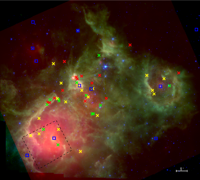
Figure 1 shows a three-color image of NGC 2467; the IRAC 4.5 m channel is in blue, the IRAC 8.0 m channel is in green, and the MIPS 24 m channel is in red. The IRAC and MIPS images show a region of ionized gas pushing out into the surrounding molecular cloud. Strong polycyclic aromatic hydrocarbon (PAH) emission can be seen in the 8.0 m band. PAH emission is present throughout the photodissociation region (PDR) at 8.0 m. PAH emission shows the locations of edges and ionization fronts created by the O star. The MIPS 24 m emission is concentrated in the area surrounding the central O6 star, indicating the presence of warm dust. The locations of the possible detected YSOs are shown in Figure 1, along with the locations of known OB stars in the region.
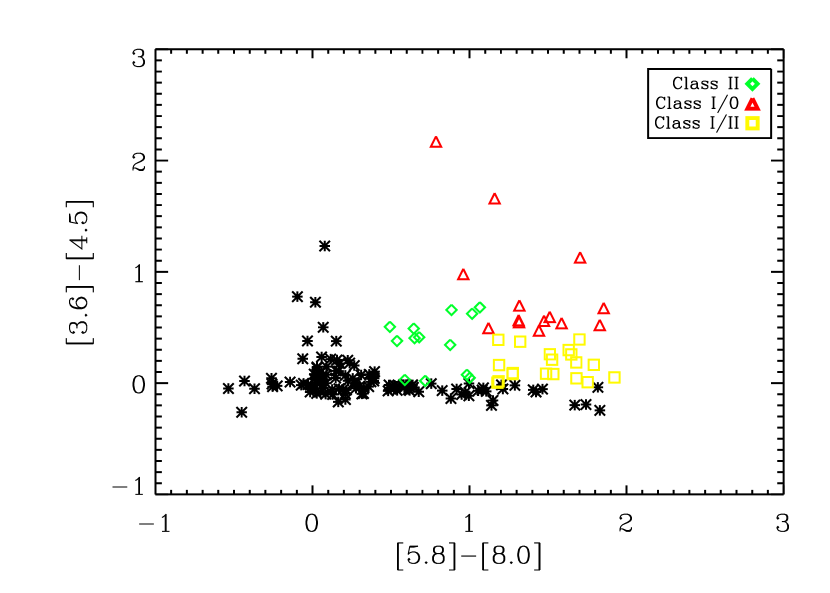
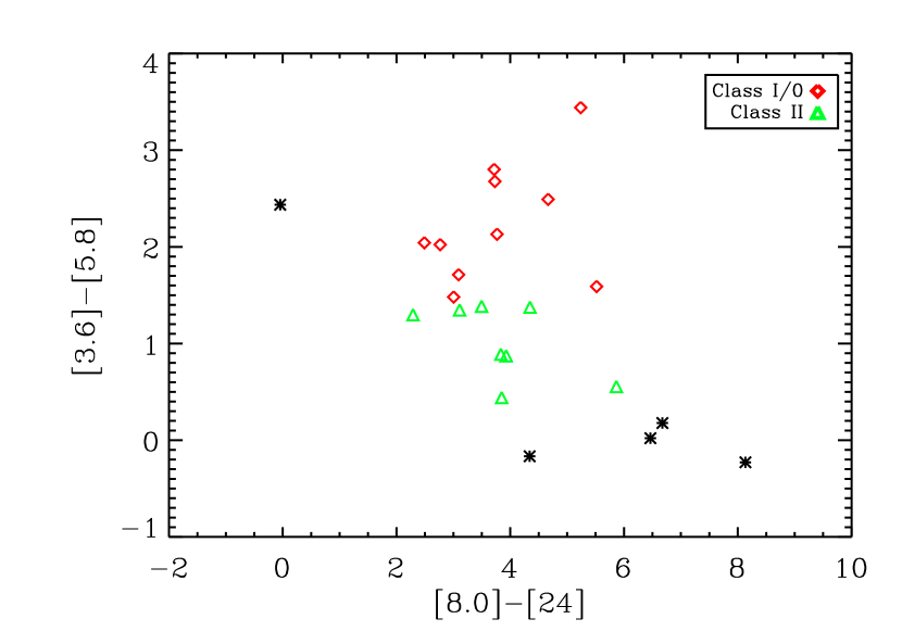
Figure 2 shows an IRAC color-color diagram of [3.6]-[4.5] vs. [5.8]-[8.0] for NGC 2467. The protostellar candidates are plotted in color in Figure 2; Class II sources are in green, Class I/II sources are in yellow, and Class I/0 sources are plotted in red. Figure 3 is a color-color diagram for the 23 detected point sources in the MIPS 24 m band, with [3.6]-[5.8] vs. [8.0]-[24]. Of these, 18 MIPS sources were classified as protostars based on their colors. Class I/0 sources are plotted in red and Class II sources are shown in green. Of the 18 MIPS 24 m sources that were found to have a mid-IR excess, all corresponded to an IRAC point source that also had a measured color excess in one or more IRAC colors. Sources that had a large color excess in the [8.0]-[24] color, but a [3.6]-[5.8] color less than zero, are defined by Reach et al. (2004) as sources with possible debris disks. Four 24 m sources fell into this color regime. There are 45 sources from both the IRAC and MIPS color-color diagrams that had an infrared excess in at least two colors, and 18 sources had a measured color excess in four different colors.
Fourteen IRAC and 10 MIPS sources were found to have colors indicative of Class I/0 objects. Models of objects with these colors from Allen et al. (2004) and Whitney et al. (2003a, 2003b 2004b) correspond to protostellar objects with infalling dusty envelopes. These are the youngest objects in the sample. Of the 10 MIPS Class I/0 sources, four corresponded to IRAC Class I/0 objects, and six corresponded to IRAC Class I/II sources. Thirteen IRAC and 8 MIPS sources were found to have colors indicative of Class II protostellar objects. The colors of these objects are characteristic of models of young low-mass stars with disks (Allen et al. 2004 and Whitney et al. 2003a, 2003b 2004b). These objects are more evolved than the Class I/0 objects. Two MIPS Class II sources correspond to an IRAC Class II, and five of the MIPS Class II sources correspond with an IRAC Class I/II source. The other MIPS Class II source corresponds to an IRAC Class I/0 source. Eighteen other IRAC sources were classified as Class I/II objects based on their colors. The MIPS classification of YSOs overlapped fairly well with the IRAC classification. Cases where the sources did not correspond are mostly due to the fact that we only had two separate classifications of MIPS sources, but three possible classes for the IRAC sources.
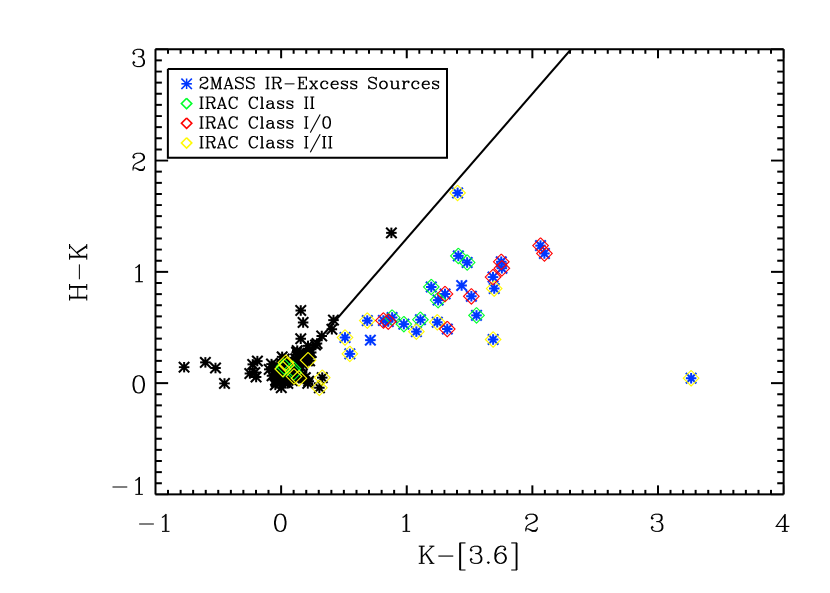
Figure 4 shows a 2MASS Spitzer color-color diagram of the 2MASS detected sources. The 29 sources to the right of the reddening vector are highlighted in blue, indicating an infrared excess in their 2MASS colors. The reddening vector due to interstellar extinction has a slope of 1.3 as defined by Tapia (1981). The corresponding IRAC YSO candidate sources are also identified; 27 of the 29 2MASS sources with an infrared excess correspond to YSOs selected from Spitzer. There is some separation of the IRAC classified sources seen in the 2MASS color-color diagram. A large fraction of the IRAC Class I/0 objects are the reddest sources in the K-[3.6] color. The IRAC Class II objects lie in the middle range of color excess for the K-[3.6] color, but most have higher H-K colors than the Class I/II objects.
4. Discussion
4.1. SED Model Fitting of YSOs
We are interested in determining the masses, ages, and other physical properties of the detected YSOs. To constrain the physical properties of each of the 45 YSO candidates we used an online SED fitter from Robitaille et al. (2007). The fitter uses a grid of SEDs corresponding to various YSO / disk models, generated by radiative transfer codes from Whitney et al. (2003a, 2003b 2004b); for each YSO/disk model, SEDs are presented at 10 different inclination angles of the disk to the line of sight, equally spaced in intervals of cosine of the inclination, giving 2105 total SEDs. There are 14 different parameters characterizing a YSO/disk model, including stellar mass, age, temperature, and radius, as well as disk mass, envelope accretion rate, and other properties. Assumed stellar masses range from 0.1-50 M⊙, stellar ages range from , photospheric temperatures range from 2535 - 46000 K, and stellar radii range from 0.4 - 780 R⊙ in the models The parameters comprising the grid of models are distributed so that there is a uniform density of models in , and close to a uniform density of models (there is a slight bias towards larger values of stellar age). The reader is referred to Robitaille et al. (2006) for more details on the total range of parameters.
The SED fitter from Robitaille et al. (2007) can help determine the uniqueness of a given fit based on the best-fit (reduced) value of a model and on the range of values for the various parameters in the model fits. Numerous recent Spitzer studies have successfully used this fitter in identifying and classifying YSOs. Simon et al. (2007) used the online SED fitter to identify YSOs in the ii region NGC 346 in the Small Magellanic Cloud (SMC). Other recent work by Poulton et al. (2008) has used the SED fitter to model detected YSOs in the Rosette Nebula; they were able to identify over 750 YSOs and classify their evolutionary state. Seale and Looney (2008) used the SED fitter to look at the evolution of outflows produced by nearby YSOs. They found that the SED fitter from Robitaille et al. (2007) adequately matches the observed data from their sample of 27 YSOs.
For NGC 2467, the Spitzer and 2MASS fluxes for each candidate YSO were input into the SED fitter, along with a distance estimate for the region. All of our 45 candidate YSOs had at least four flux measurements, with the majority (39 out of 45) having seven or eight flux measurements. The fitter outputs a set of models for each source, and only models with (per data point) were used in our analysis in determining the best-fit properties of each candidate YSO (similar to methods used by Robitaille et al. 2007 and Simon et al. 2007). We selected models that had ages less than 2 Myr, i.e. only models with ages that are within the assumed age of the region. We calculated the average mass only from models that were within 3 sigma of the total 2 from the best-fit. The

corresponding model with the lowest 2 and mass closest to the weighted average mass was used. All of the candidate YSOs were checked against pure stellar photosphere models, and the total of the stellar fit was compared to the from the YSO fits. None of the candidate YSOs was better fit by a pure stellar photosphere model, confirming our color selection criteria of YSOs for this region. The YSO best-fit parameters for each source are listed in Table 4. We found sources with masses ranging from 0.35 - 5.7 M⊙ and ages ranging from 103 - 1106 yr. There were at least seven sources that had a best-fit mass of less than 1 M⊙, demonstrating that we are detecting some fraction of the low-mass protostellar population.
4.2. Mass Distribution of YSOs and Completeness
A mass estimate for each of the candidate YSOs allows for an examination of the overall population of sources in this region. In order to look at the distribution of masses of YSOs in NGC 2467 and to estimate completeness, we used the best-fit model masses to determine a mass function for the 45 sources. We assumed a mass function of the following form:
| (1) |
Figure 5 shows a histogram of YSOs as a function of their best-fit mass. The masses of the 45 YSOs were grouped into 6 equally spaced mass bins, centered at 0.5, 1.5, 2.5, 3.5, 4.5, and 5.5 M⊙. Various least-squares fits were performed on the data in order to determine the exponent above. As is apparent from Figure 5, the deviation from a single power law becomes progressively worse at small mass bins, indicating an incompleteness in our survey. Our first fit (#1) is fit only to the two most complete mass bins (at 4.5 and 5.5 ), and yields a slope of (where the error estimate includes only the error associated with these small-number statistics). Our second fit (#2) is fit to the three highest mass bins (3.5, 4.5 and 5.5 ), and yields a slope of . The first fit, using only the highest mass bins, is definitely compatible with a Salpeter (1955) initial mass function (IMF) with slope , which we adopt here.
Our survey is probably close to complete in the two highest mass bins, but probably partially incomplete in the 3.5 mass bin, and increasingly incomplete in lower mass bins. A power-law fit, it should be noted, probably is not appropriate for the lowest mass bins below , which might more appropriately be modeled with a log-normal distribution (Chabrier 2003). This is not relevant to the current study, however, which seeks only to judge the total number of stars forming in the region, and not so much the exact shape of the IMF.
| Source | Model | Mass | Age | Radius | Temp | AV | Log(d) |
|---|---|---|---|---|---|---|---|
| (M⊙) | ( 105 yr) | (R⊙) | (K) | (mag) | (kpc) | ||
| 1 | 3011772 | 2.10 1.17 | 1.00 | 10.98 | 4340.0 | 5.3 | 0.61 |
| 2 | 3003476 | 3.59 1.25 | 0.09 | 21.63 | 4298.0 | 0.6 | 0.62 |
| 3 | 3004748 | 1.92 0.39 | 0.07 | 14.42 | 4180.0 | 3.8 | 0.62 |
| 4 | 3018503 | 0.62 0.54 | 0.14 | 6.61 | 3816.0 | 1.5 | 0.62 |
| 5 | 3012434 | 1.35 0.59 | 0.02 | 12.91 | 4050.0 | 0.0 | 0.60 |
| 6 | 3014174 | 0.99 0.31 | 0.53 | 6.81 | 4103.0 | 0.8 | 0.60 |
| 7 | 3010612 | 0.93 0.29 | 0.24 | 7.54 | 4027.0 | 20.3 | 0.61 |
| 8 | 3009627 | 2.46 1.31 | 0.78 | 12.66 | 4359.0 | 4.0 | 0.60 |
| 9 | 3011577 | 1.23 0.44 | 0.04 | 12.89 | 3995.0 | 4.3 | 0.62 |
| 10 | 3008298 | 1.52 0.75 | 0.05 | 12.33 | 4124.0 | 22.7 | 0.61 |
| 11 | 3016995 | 0.63 0.57 | 4.70 | 3.66 | 3936.0 | 1.4 | 0.61 |
| 12 | 3015705 | 0.35 0.46 | 0.61 | 3.72 | 3489.0 | 2.4 | 0.60 |
| 13 | 3006942 | 2.52 1.04 | 0.22 | 14.76 | 4305.0 | 0.2 | 0.62 |
| 14 | 3010799 | 1.43 0.90 | 0.38 | 8.76 | 4226.0 | 2.3 | 0.62 |
| 15 | 3005834 | 2.37 1.33 | 0.56 | 12.61 | 4343.0 | 0.0 | 0.60 |
| 16 | 3007424 | 4.70 0.33 | 12.00 | 2.68 | 16000.0 | 0.1 | 0.62 |
| 17 | 3008715 | 3.94 0.93 | 4.00 | 8.24 | 4903.0 | 0.0 | 0.60 |
| 18 | 3003892 | 4.31 0.50 | 6.60 | 9.46 | 5762.0 | 5.3 | 0.60 |
| 19 | 3016713 | 1.16 0.35 | 0.02 | 11.81 | 4008.0 | 0.0 | 0.60 |
| 20 | 3017850 | 2.50 0.87 | 4.40 | 5.73 | 4700.0 | 1.0 | 0.62 |
| 21 | 3009574 | 1.98 1.57 | 0.61 | 10.93 | 4313.0 | 0.0 | 0.60 |
| 22 | 3005274 | 5.73 0.26 | 2.90 | 14.27 | 6109.0 | 10.4 | 0.61 |
| 23 | 3016205 | 3.80 1.00 | 3.20 | 8.62 | 4807.0 | 0.0 | 0.60 |
| 24 | 3010603 | 1.10 0.88 | 5.30 | 3.59 | 4314.0 | 1.2 | 0.60 |
| 25 | 3005254 | 2.55 0.41 | 0.86 | 12.85 | 4369.0 | 1.8 | 0.61 |
| 26 | 3016360 | 1.88 0.11 | 1.10 | 10.02 | 4321.0 | 0.1 | 0.62 |
| 27 | 3002399 | 0.89 0.69 | 0.14 | 7.86 | 3989.0 | 3.2 | 0.60 |
| 28 | 3017155 | 2.44 1.94 | 0.28 | 13.77 | 43190.0 | 0.0 | 0.60 |
| 29 | 3018885 | 1.92 1.02 | 0.92 | 10.39 | 4318.0 | 7.3 | 0.60 |
| 30 | 3005897 | 2.17 0.85 | 0.94 | 11.39 | 4341.0 | 0.0 | 0.60 |
| 31 | 3017257 | 1.23 0.27 | 0.11 | 11.08 | 4057.0 | 22.4 | 0.62 |
| 32 | 3006533 | 4.21 0.14 | 5.40 | 9.21 | 5209.0 | 0.0 | 0.60 |
| 33 | 3011105 | 3.15 0.92 | 1.30 | 12.49 | 4502.0 | 1.0 | 0.62 |
| 34 | 3000825 | 4.17 0.12 | 8.30 | 8.33 | 6482.0 | 0.0 | 0.60 |
| 35 | 3011935 | 0.83 0.33 | 0.19 | 7.14 | 3976.0 | 4.2 | 0.61 |
| 36 | 3000455 | 1.28 0.94 | 1.10 | 7.66 | 4214.0 | 2.0 | 0.60 |
| 37 | 3012794 | 4.21 0.21 | 5.70 | 9.26 | 5268.0 | 1.8 | 0.60 |
| 38 | 3005266 | 5.12 0.11 | 5.70 | 7.81 | 9534.0 | 5.9 | 0.61 |
| 39 | 3016265 | 3.81 0.78 | 9.20 | 7.91 | 5612.0 | 0.7 | 0.60 |
| 40 | 3005266 | 5.12 0.56 | 5.70 | 7.81 | 9534.0 | 6.9 | 0.62 |
| 41 | 3015096 | 1.40 0.67 | 2.00 | 7.05 | 4292.0 | 1.5 | 0.61 |
| 42 | 3019036 | 3.62 0.95 | 0.59 | 17.12 | 4414.0 | 1.2 | 0.62 |
| 43 | 3005949 | 3.99 0.45 | 10.00 | 7.18 | 7158.0 | 5.5 | 0.62 |
| 44 | 3011228 | 2.90 1.22 | 0.07 | 19.35 | 4246.0 | 12.6 | 0.62 |
| 45 | 3010779 | 2.55 0.80 | 1.00 | 12.55 | 4386.0 | 2.1 | 0.62 |
There are approximately 20 known B8 and B9 stars in the region from cluster surveys of H19, H18, and SH-311 (Moreno-Corral et al. 2002). There are also two known O stars (O6 and O7) associated with the region. The number of B8/B9 stars was used to fix the IMF normalization constant above, assuming a mass range of ; using the two known O stars (and a mass range of also gives us a very similar normalization constant. The calculated average value of the normalization constant is , again assuming Poisson statistics on the 20 B9/B8 stars. We therefore estimate the total number of stars between and in NGC 2467 to be
| (2) |
In order to address completeness, we estimate the total fraction of YSOs that should have been detected in this sample. Using the flux limits from our Spitzer observations, we calculated the fraction of the total 200,000 SED models from Robitaille et al. (2006) that we would have been able to detect. Our calculated flux limits were based on our three-sigma magnitude limits for the IRAC bands for our observations: 14.3, 14.1, 12.4, and 11.6 mag for IRAC 3.6, 4.5, 5.8, and 8.0m, respectively. The SED models in the grid are based on sources at 1 kpc, so the model fluxes were scaled to 4 kpc, the assumed distance of our sources. The extinction to this region ranges from 1 - 3 magnitudes in AV with an average extinction of AV equal to 2 magnitudes (Moreno-Corral et al. 2002 and Munari et al. 1998); this average AV was also accounted for in the flux limits. We found that with our flux limits we should have been able to detect 42 of all models in the grid. This detection limit is based on our minimum flux limits in the high background areas, and therefore applies to the fraction of objects we should detect in the regions of higher nebular emission.
4.3. Comparison to HST Images
The main motivation of our Spitzer proposal was to observe a select number of ii regions with Spitzer that had already been observed with HST. HST images provide us with detailed information about YSOs after they are in an ionized ii region environment, whereas Spitzer allows us to see both a larger view of the region and also to see protostars and their disks that are still embedded in the dense gas around the ii region.
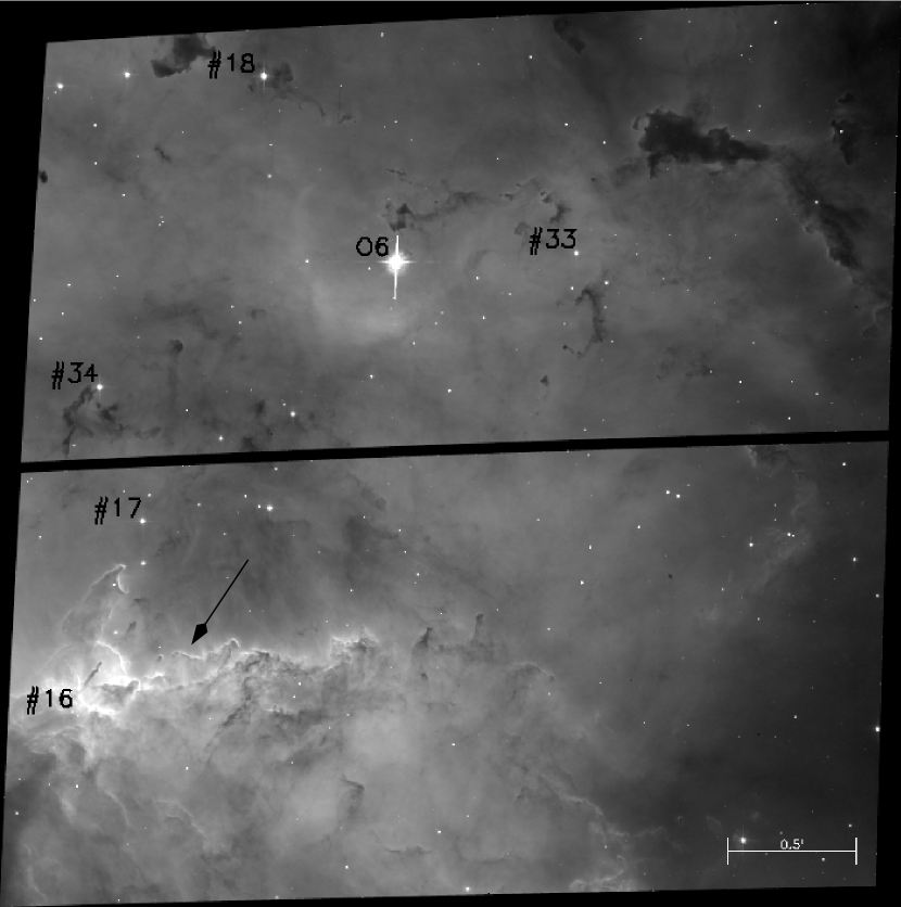
The HST ACS images of NGC 2467 by De Marco et al. (2006) were combined with our Spitzer images in order to compare what is seen with the different wavelength regime and better resolution of HST with the larger field of view of the Spitzer images. The HST field is centered around the O6 V star, the brightest object in the HST ACS image, and a number of fragments, globules, and ionization front edges are also seen in these images. Five Spitzer-detected YSOs are located in the HST field: three Class I/II sources and two Class II sources. Including the five YSOs, only a total of eight point sources were detected in all four IRAC bands meeting our flux criteria set by the high background emission and fall in the ACS FOV. There are, however, more than eight point sources seen in the ACS image, as well as in the two shorter wavelength IRAC bands in the ACS FOV. The HST ACS H image of NGC 2467 is shown in Figure 6; the five detected YSOs are labeled in the image by their YSO source number; the O6 V star is also labeled. Source 16 is classified as an IRAC Class I/II source and a MIPS Class I/O source, with a best-fit mass of 4.70.3 M⊙ from our SED fitting. Source ’s 17 and 18 are IRAC Class I/II sources with masses of 3.90.9 M⊙ and 4.30.5 M⊙, respectively. Source ’s 33 and 34 are IRAC Class II sources with masses of 3.20.9 and 4.20.1 M⊙, respectively.
Four out of the five YSOs (’s 16, 18, 33, and 34) in the HST field are seen sitting against or near to dark clumps in the ACS image. There appears to be one main ionization front that
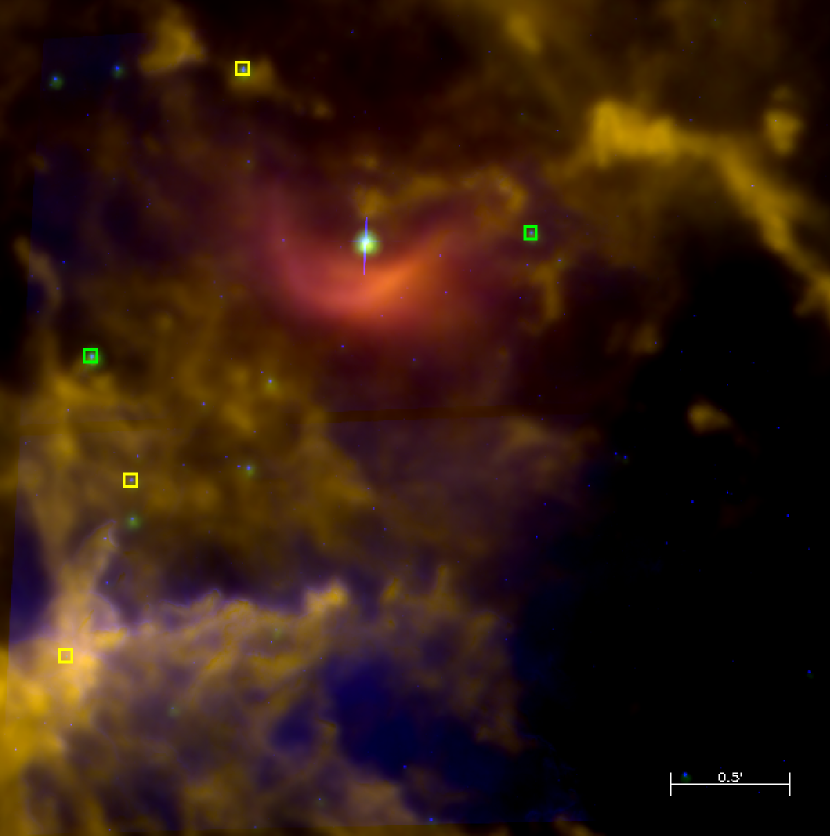
can be identified in the HST image, located to the bottom left of the image (see arrow in Figure 6). This location corresponds to a column of gas seen in the Spitzer images where a large number of YSOs are located. Figure 7 is a three-color HST and Spitzer image of the region with the Spitzer data scaled to the HST field of view. The ionization front from the main column in the Spitzer bands is clearly outlined by the ionization front as seen in the F658N filter. Three YSOs appear to be in close proximity to this ionization front in the HST field. De Marco et al. (2006) make note of the many fragments that are being uncovered by the advancing ionization front. Two of the Spitzer sources (’s 17 and 34) close to this ionization front appear to already have been uncovered and are now sitting in the interior of the ii region. The third source located in close proximity to the ionization front, 16, is somewhat more confusing as it appears to be embedded in one of these fragments, as viewed in Figures 6 and 7. The source is also somewhat hard to see in the ACS image in Figures 6 and 7, but when viewed at full resolution in the ACS image there is a possible faint identifiable point source present. It also has a small best-fit extinction value (AV = 0.1). Therefore, it is plausible that source 16 has also recently been uncovered from the passing ionization front. One of the other YSOs, 18, at least in projection appears to be located in a denser clump of material which can be seen in the F656N HST image. It does have a larger extinction value as best-fit from the SED modeling with AV equal to 5.3, but the point source is clearly visible in the ACS image. So, again it is hard to conclude if this source is still embedded in the dense clump of material as seen in Figure 7, and may likely have already been uncovered. The fifth YSO in the HST field is source 33; it is close to the O6 V star, and it also appears to be sitting inside the ii region.
One note of interest is that two of the Class I/II sources (’s 16 and 18) which are less evolved are possibly embedded sources, or are at least seen sitting against dense clumps of material. In contrast, the two Class II sources (’s 33 and 34) that are presumably more evolved are located in the interior of the ii region, and have already been uncovered by the ionization front from the O6 star. Source 17 is a Class I/II and it appears to also be located in the interior of the ii region, but it is very close, within 0.2 pc, to the edge of the ionization front and to a dense finger of gas. We interpret this as meaning that it has recently been uncovered by the ionization front. This shows that even in the HST field alone, without detailed analysis, we already see a progression of younger sources still embedded in the dense gas waiting to be uncovered by the advancing ionization front, and older Class II type sources sitting inside the ionized ii region having already been uncovered by the ionization front.
4.4. Spatial Distribution
If there is no triggering occurring and the formation of most YSOs is independent of the effects of the massive stars and ii region expansion, then we would expect that the spatial distribution of YSOs would not be correlated with compressed gas or ionization fronts. If this is the case, then we would expect to see clusters of low-mass stars already forming in the outer regions around ii regions. On the other hand, if there is a significant fraction of triggered star formation in ii regions, then we would expect to see the distribution of YSOs concentrated in the compressed gas and nearby to ionization fronts (see figures 8 9 from Hester Desch 2005 for a more detailed explanation of these scenarios and the observational signatures of each).
We are interested in using our data to quantitatively distinguish between these possible scenarios, triggered vs. non-triggered, coeval star formation, or determine if there is a combination of these modes occurring. One possible way to do this is to look at the distribution of protostellar sources in the region; if they are all coeval then we would expect the YSOs to be distributed the same way as all other sources, including the more massive OB stars. If triggering is occurring, we also want to estimate the mechanism of triggering from the expansion of the ii region.
As discussed in the introduction, there are a number of predictions for the three different proposed scenarios. For all three models, one expects to see a correlation between the locations of the protostars and the ionization and shock fronts. For RDI, we expect no protostars to be forming in front of the ionization front, as it is the high pressure from the ionized gas that causes the clumps to implode. For “collect and collapse”, we expect to see regularly spaced protostars within the swept-up, compressed material. For the third scenario, where triggering occurs from the shock front traveling in advance of the ionization front, one expects to see the youngest protostars in the compressed gas between the shock and ionization fronts, and to ages of protostars correlated with distance from the ionization front. We tested these scenarios and triggered star formation vs. coeval star formation by comparing the YSO distribution to the OB stellar population distribution and to the location of ionization fronts in NGC 2467.
4.4.1 Ionization Front Detection
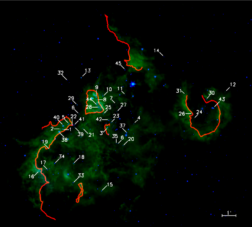
Ionization fronts were identified first coarsely, by examining the images by eye, and then more precisely by running the edge detection routine, roberts.pro in astrolib of IDL, on the 5.8 and 8.0 m band images. This routine performed gradient or directional filtering, selecting locations where the pixel values changed by a large amount from one pixel to the next in a given direction. Six areas in NGC 2467 had sharp edges visible in the smoothed image produced by the edge detection routine and these 6 areas were determined to contain possible ionization fronts. Once the six main ionization fronts were identified, they were mapped in xy coordinates using a routine in IDL that returns coordinate values; this routine yielded an x and y position along the length of each ionization front. The thickness of each ionization front outlined in the images of NGC 2467 was assumed to be 1017 cm thick, comparable to typical thicknesses of ionization fronts (1016 - 1017 cm; Osterbrock 1989). Figure 8 shows the locations of all 45 YSOs, labeled by number, and the identified ionization fronts (on the same scale as in Figure 1). The identified ionization fronts are outlined in red and over-plotted on the IRAC 8.0 m band in green and the IRAC 4.5 band in blue.

The main ionization front identified is around the column on the left of the image, as seen in Figures 1 and 8. The O6 V ionizing star is near this column of gas; it has an average projected distance of 3 pc away from the column. Seven protostellar sources (’s 1, 2, 5, 16, 22, and 40) were identified in projection on this column, along with three additional sources (’s 19, 39, and 41) which appear, in projection, to be just past the ionization front presumably having recently been uncovered. All ten sources are very near (1-18′′) to the edge of the ionization front. Assuming a distance of 4.1 kpc to NGC 2467, these 10 sources are located at projected distances ranging from 0.02 to 0.35 pc from the edge of the ionization front. The second region with an ionization front and a strong clustering of sources is the central cluster in the middle of the image. This region is dominated by strong emission from a few B stars in H18ab, the most massive is a B1 V star. There are a large number of detected YSOs near this sub-region, with the eight closest protostellar sources (’s 6, 8, 9, 10, 25, 28, 29, and 44) having projected distances from this ionization front ranging from 0.12 to 0.73 pc.
The third most noticeable region is towards the upper right of the image; this region is excited by the B1 V star in the H19 cluster. The presence of a possible Strmgren sphere around this cluster of stars was revealed by narrow-band H, [N ii], and [S ii] from Moreno-Corral et al. (2002). The ionization front at the edge of this possible Strmgren sphere is clearly defined in the Spitzer images of NGC 2467. There are five protostellar sources (’s 24, 26, 30, 31, and 43) sitting right near the edge of the ionization front, with projected distances from the ionization front ranging from 0.03 to 0.50 pc. There is also one other source (12) slightly farther out, at a projected distance of 1.04 pc.
Three other ionization fronts were identified using the edge detection routines. Another five detected YSOs (’s 3, 23, 33, 42, and 45) are located in close proximity to these three ionization fronts. Overall, 29 of the 45 identified YSOs appear strongly clustered around the detected ionization fronts, which demonstrates that the majority of the detected YSOs are most strongly concentrated around the ionization fronts, and they are not well correlated with the O and B star locations.
The histogram distribution of source distances shown in Figure 9 shows that there is a markedly higher frequency of sources near the ionization fronts. The projected distances of the 45 YSOs from the nearest ionization front ranges from 0.02 - 2.2 pc, with more than 60 (28 out of 45), of the sources falling within 0.6 pc of a detected ionization front, and 70 (32 out of 45 objects) falling within 1.0 pc of an ionization front. Our analysis is incapable of detecting face-on ionization fronts; therefore the other 13 sources, which are not seen in projection within 1.0 pc of an ionization front, may still be near ionization fronts as well.
4.4.2 Distribution Tests
The average projected distance of the edge-on ionization fronts in NGC 2467 is about 3 - 5 pc away from the OB stars. A simplified 3D-model111A cylindrical bowl, with equal height and width was used to model the distribution. of a hemispherical ionization front which is on average 3 to 5 pc away from an O star was compared to the distribution of sources we see in NGC 2467. This model was used in order to determine if it is likely that the other YSOs not seen in projection within 1 pc from an ionization front are in fact closer to the ionization front than they actually appear to be. We were only able to detect parts of the ionization fronts that are moving edge on to our line of sight. However, we would not be able to detect the part of the ionization front that is face-on. We therefore want to determine where this total predicted distribution of sources matches the observed distribution of YSOs in NGC 2467.
In order to calculate the predicted distribution of sources within a layer a given distance away from the ionization front, we calculated the ratio of the edge-on volume of this distribution (which we would be able to observe) to the total volume of this distribution. The thickness of the expected YSO distribution was measured from 0.1 to 2.2 pc. As the thickness of the distribution increased, the larger the percentage of expected observed sources within that distribution layer becomes. Varying the radius from 3 to 5 pc (the distance of ionization front to the OB star) only slightly changes the predicted fraction of sources at a given thickness. Using this model, we calculated that a distribution that is concentrated within a layer 0.5 pc away from an ionization front would show 68 of the sources within a projected distance of 0.5 pc from this layer when viewed in projection. For a distribution that is concentrated within 1 pc, we calculated that 70 or less of the sources should be seen in projection within 1 pc. However, for the actual distribution of YSOs in NGC 2467 almost 60 of them are seen in projection within 0.5 pc of an ionization front and over 70 are seen within 1 pc of an ionization front.


Figure 10 shows the predicted fractions of sources for the 3D-hemispherical model centered at 3 and 5 pc versus thickness, along with the actual fraction of YSOs that are within the same distance (thickness) from an ionization front. The observed YSO distribution crosses the predicted model fractions at a distance between 0.9 and 1.0 pc. Above a distance of 1 pc, the YSO fraction is greater than the expected distribution. This suggests that the overall distribution of YSOs in NGC 2467 is a population of sources that is concentrated within a layer that is 1.0 pc or less away from an ionization front.
A second statistical method was used in order to test the likelihood of this current distribution occurring. We calculated the probability of the YSO sources being randomly distributed versus the actual observed distribution. We calculated the fraction of the survey area that is within a given distance of the ionization fronts. If this is a random distribution then we would expect the fraction of YSOs located within a given distance of an ionization front to equal the fraction of the total survey that is within that distance. For example, only 4 of the survey area is within 0.2 pc of an ionization front, but 10 out of 45 YSOs (22) are located within this distance. The probability of 22 of all randomly distributed YSOs falling within 0.2 pc of the ionization front by chance is only 0.001. This was calculated using a Poisson probability distribution, which gives the probability of a specific number of YSOs (k) being distributed randomly, as shown by Equation 3:
| (3) |
The expected number of sources () is equal to the fraction of the survey area within a given distance multiplied by the total number of sources (45) and k is equal to the observed number of YSOs within that distance. The probability of a random distribution drops to as low as 10-12 at a distance of 0.5 pc from the ionization front, where 26 out of 45 YSOs are located within this distance, despite only 11 of the total survey area being within this distance. Looking at the likelihood of all 45 YSOs being located within a distance of 2.2 pc of the ionization fronts, we find the odds of this occurring by chance to be 10-6. Therefore, we conclude that this is not a random distribution of sources. The data indicate that the locations of YSOs are strongly correlated with the location of the ionization fronts.
4.4.3 Distance and Age with Evolutionary Class
We also examined the distribution of YSOs for each specific evolutionary class in order to determine if there is any noticeable trend in distance from ionization fronts versus evolutionary class, and to also help in determining how the triggering might be occurring. If RDI is occurring, we expect no protostellar objects to be located ahead of the ionization front because in this scenario the high pressure ionized gas leads to the implosion of pre-existing clumps. For the other two scenarios, the shock front preceding the ionization front triggered the collapse. The youngest protostars will be located in the compressed gas between the two fronts, and there should be an age progression with distance from the ionization front.
For this analysis, we looked at the distance of each YSO from the ionization front in terms of those already uncovered versus those still embedded. YSOs that appear to be ahead of the ionization front and are still embedded are considered to have a negative distance from the ionization front. YSOs that are behind the passing ionization front and have already been uncovered are given a positive distance. Figure 11 shows a histogram of the distance of the Class II and Class I/0 YSOs from the nearest ionization front, with positive distances for YSOs behind the front and negative distances for those ahead of the ionization front. In this plot it is fairly clear to see a separation between the two different types of YSOs. The majority of the Class II YSOs have already been overrun by the passing ionization front (10 out of 13 with positive distances), and on the other hand a majority of the Class I/0 YSOs (10 out of 14 with negative distances) are still embedded in compressed molecular gas and have yet to be uncovered by the ionization front. The Class I/II YSOs, which are not plotted in Figure 11, fall in between these two distributions, with two-thirds (12 out of 18) located behind the front, and the other third still embedded in compressed gas ahead of the ionization front. This suggests that we see a trend of evolution with distance from an ionization front.
We can also rule out RDI as a dominant mechanism for triggered star formation in this region because we do see a number of protostellar objects located ahead of the ionization front, suggesting that the YSOs are being triggered from the shock front traveling in advance of the ionization front. We favor the shock front traveling in advance of the ionization front as the triggering mechanism over the “collect and collapse” scenario because we do not see strong evidence for regularly spaced protostars forming around the edge of the ii region. We also see strong evidence, as shown in Figure 11, for a distribution of YSOs with ages that correlate with distance from the ionization front. However, it is still plausible that some YSOs in this region formed by the “collect and collapse” mechanism as well. The third triggered star formation scenario can also account for why we see a lack of protostars close to the OB stars, ie.) between the O star and the ionization fronts. This gap exists because we cannot directly observe stars older than a certain age with this dataset, those that would be located nearest the OB stars. Either no other stars formed near the OB stars, which does not seem plausible, or stars formed near the OB stars first and all the new protostars forming now are spatially correlated with the ionization fronts. Therefore the lack of new protostars currently near the OB stars, and the correlation of new protostars with the ionization fronts, over wide spatial scales in the region, is direct evidence for a triggering mechanism.
An argument against the triggered star formation scenario is that many of these objects may have been forming before the shock front passed over them. In this case, they are just being uncovered by the passing ionization front, and not triggered by the compression of the molecular gas due to the expanding shock front. This therefore partly becomes an age argument; if the majority of the sources have ages much greater than the timescale between the passage of the shock front and the ionization front, then it would be possible that they were forming before the shock front compressed the surrounding molecular gas. The passage of the shock front is typically followed by the passage of the ionization front within a few105 yr (Hester and Desch 2005; Sugitani et al. 2002).
For the 32 sources that fall within a projected distance of 1 pc or less from an ionization front, 70 have best-fit ages less than or equal to 105 yr and 80 have ages less than 3105 yr. For all 45 YSOs, 65 have ages less than or comparable to the timescale between the passage of the shock front and the ionization front. Although the SED model best-fit ages may not be completely reliable, we can also use the calculated distances of the YSOs from the ionization fronts and can compare the time elapsed since the ionization front passed the YSOs (or will pass them) to their lifetimes. Assuming an ionization front speed of 0.5 - 2 km s-1 (Osterbrock 1989), sources at a projected distance of 0.5 pc from an ionization front are only 2.5 105 - 1106 yr away from the nearest ionization front. YSOs that are closer than 0.5 pc were passed by the ionization front even more recently (or will be uncovered by the advancing ionization front even sooner). These timescales are comparable to the best-fit ages and expected lifetimes of Class 0, Class I, and Class II protostellar objects. We conclude that we are seeing very young objects that are still forming, many that are even younger than 105 yr. This demonstrates that when the majority of the YSOs formed in the last few105 yr they likely formed in gas compressed by the shock front from the expanding ii region, and are now forming very near to ionization fronts.
The most notable thing we see with the distribution of these sources is that they are strongly associated with the ionization fronts, and they are not randomly distributed. We also do not see clustering of YSOs around the OB stars, which seems to suggest that they are not correlated with the distribution of the OB stars themselves, but are instead more correlated with the ionization front locations. Also, we see no discernible separation in the distribution of the low-mass and the intermediate mass YSOs from the ionization fronts. It appears that low-mass sources are just as likely to be triggered by the expansion of the ii region as the more massive YSOs. Therefore it appears that the star formation is not strictly coeval in NGC 2467, and that triggered star formation due to the expansion of the ii region is occurring. Overall, the distribution of the candidate YSOs in this region suggests that a clear majority of the current protostars are forming in regions of gas that are being compressed from the advancing shock and ionization fronts.
4.5. Estimates of Triggering and Star Formation Rates
A final way to test the various scenarios for star formation in this region is to estimate the amount of triggering that has occurred in NGC 2467 throughout the lifetime of the region. First, we estimate the total star formation rate (SFR) in NGC 2467. Using the Salpeter IMF, we determined that there should be a total of 5000 stellar sources ranging in mass from 0.2-40 M⊙(see equation 2). We calculate the total mass in stars from the Salpeter mass distribution (Salpeter 1955), giving a total of 3500 M⊙, as shown in Equation 4. From there, we calculate the average SFR in NGC 2467 over the last 2 Myr, given by Equation 5:
| (4) | |||||
| (5) |
In §4.2, we showed that from our Spitzer flux limits we should be able to detect 42 of all YSO sources based on the grid of SED models from Robitaille et al. (2006), however this estimate disregarded the age of the sources and age of the region. Therefore, in order to calculate the total triggered star formation rate, we want to measure how the detection ability of individual sources would change with elapsed age in the region and age of the individual source. We want to include only realistic models, because the fraction of detectable sources depends on the number of models we compare to. To do this, we took a population of stars given by the Salpeter IMF, between our mass limits of 0.2 and 40 M⊙, and assumed a constant SFR equal to the average SFR from Equation 5 (1.7510-3 M⊙ yr-1), and then used the Salpeter IMF to age that population of stars. We looked at the detection probabilities for this population of stars at timesteps every 105 yr. During each timestep we would take the population of stars at that specific age and of various masses (determined by the IMF), and determine the percentage of sources, from the SED models, we should detect based on our Spitzer flux limits. The population of stars was aged from one timestep to the next, with a new population of young stars added in at each timestep.


In Figure 12 we show the fraction of detectable objects versus age of the individual sources. In this plot, we see that the best range of ages to detect the YSOs is from 0.1 to 0.5 Myr, and the peak age is at 3105 yr. After 0.5 Myr, the detection rate drops off dramatically. Within the first 0.5 Myr, the fraction of detected sources is near 50, but by the time the YSOs reach an age of 2 Myr, the fraction that would be detected has fallen to less than 15. This implies that the YSOs we are detecting likely have ages of a few105 yr, agreeing with best-fit ages from the SED fitter and timescales from the ionization fronts.
In Figure 13 we have plotted detection probability vs. elapsed age of the region, with probabilities being calculated every 105 yr. This plot shows the detection rate of YSOs integrated over the star formation history of the region. During the first 0.5 Myr the detection rate was almost 50, which is comparable to the total completeness estimates of 42 that we found in §4.2; but as the age of the region increases and the population of stars ages, our detection rate decreased to only 27 by 2 Myr.
One other factor that could decrease our detection ability is the fact that once the ionization front overruns the newly forming protostar it will quickly begin to erode the protostellar disk. Johnstone, Hollenbach and Bally (1998) calculated that the disk mass loss rate for low-mass stars due to nearby massive stars is 10-7 M⊙ yr-1. Strzer and Hollenbach (1999) show that for sources in Orion at distances greater than 0.3 pc from the ionizing source, the disk mass loss rate is dependent on the initial size of the disk and the distance from the ionizing source. A recent study of disk survival in NGC 2244 using Spitzer data (Balog et al. 2007), has also shown that it is possible that effects from high-mass stars on disk survival is only limited to distances of 0.5 pc or less from the high-mass stars. Therefore, this disk mass loss rate may not be as strong in NGC 2467 as it was modeled for stars in the Trapezium Cluster; however, we are still interested in how disk photoevaporation can effect our detection abilities of YSOs located within close proximity to the ionizing sources in this region. This effect may be one reason why we do not detect more protostars located at very nearby distances to the massive stars.
Using the same method as above, with the weighted grid of models according to the calculated IMF and SFR, we looked at what fraction of sources would still be detected if the disk mass was decreased after the source was uncovered by an ionization front. Again, we want to consider realistic models, therefore we consider only models which have an initial disk mass of 10-8 M⊙ or greater. Including all models from the YSO SED grid would lower the total fraction of detectable sources. However, by setting a minimum disk mass and a minimum mass of the object (0.2 M⊙) we do not bias ourselves towards a lower, unrealistic fraction of detectable sources. The effect of different model disk masses on the detection calculations was tested by varying the lower limit of the initial disk mass from 10-9 - 10-7 M⊙. We found that the detection fractions only changed by a few percent between these different initial disk mass values, therefore the average value of 10-8 M⊙ for the minimum disk mass was used. Photoevaporation of the “EGG” and proplyd phases will be relatively short-lived stage, 104 yr during each phase (Hester Desch 2005), ending with disks typically eroded down to sizes of 30 - 50 AU. Photoevaporation of the rest of the truncated disk will take several million years (Johnstone et al. 1998). We therefore assume, for simplicity, that the majority of the photoevaporation takes place on timescales of few104 yr (Hester Desch 2005). Under these assumptions, we found that the detection rate for sources in close proximity to the ionizing source could drop from the initial 45 to as low as 17, and again the best age range to detect these objects is around a few105 yr. These data are also shown in Figures 12 and 13.
Another note of interest, as seen in Figures 12 and 13, is that while we assumed a constant star formation rate over the lifetime of the region the detection rate decreases with time. Haisch et al. (2001) showed that in young star forming clusters, the fraction of sources with disks decreases with age of the cluster. The results presented here seem to suggest that even though the same number of stars are being formed at each timestep, the total detection fraction is still decreasing, similar to the decrease in disk fraction measured by Haisch et al. (2001). Other recent studies have used the Haisch et al. result to justify that the star formation rate is dramatically decreasing with cluster age (Gounelle Meibom 2008). However, it seems plausible that the star formation rates in young clusters may not be decreasing as dramatically after the first few Myr as claimed by Gounelle Meibom (2008), only that the detectability of the total fraction of stars with disks decreases with time as demonstrated by Figures 12 and 13.
As shown in §4.4, we currently observe 45 YSOs, the majority of which have been influenced by the effects of ii region expansion. In order to look at the overall rate of triggered star formation, we need to estimate the average age of the current population of YSOs. From the SED model fitting, the 45 YSOs have best-fit ages that average to 2105 yr. From the previous analysis, we show that best age to detect the YSOs is 3105 yr. In §4.4.3, we also demonstrate that the due to the close proximity of a majority of the YSOs to the ionization fronts, the timescales are likely to be only a few105 yr.
Multiple methods have shown that the 45 current YSOs likely have average ages of few105 yr. While the actual detection fraction value might be somewhat uncertain, it is likely that it is at least below the 30 level, and under plausible assumptions for sources in close proximity (0.5 pc or less) to the ionizing OB stars, one might imagine that the detection fraction may be as low as 17. If our ability to detect the current population of sources is 17 - 27 compared to what it would have been during the first 0.5 Myr in the region, then this would also mean that the actual total number of current YSOs could be as much as five times larger. Therefore as shown in Equation 6, 45 detected YSOs with an average age of 2 - 3 105 yr results in 6 - 1310-4 stars formed per yr that are triggered.
| (6) | |||||
Using the Salpeter IMF this results in a triggered SFR of 4.2 - 9.010-4 M⊙ yr-1. If this rate of triggered star formation has been constant over the age of the region then by comparing this rate to the total SFR, given in Equation 6, this results in 24 - 52 of the total SFR. We therefore conclude that approximately 25 - 50 of the YSOs in NGC 2467 may have been formed due to triggering from ii region expansion.
There are a number of assumptions that have gone into this calculation: assuming a constant SFR, an estimate of the average age of the YSOs from multiple methods, and the determination of the current detection fraction of YSOs. Our assumption about the detection fraction of YSOs nearby the massive stars may be one factor that could change our triggered SFR estimate. If the current detection fraction is not adversely affected by the photoevaporation of YSOs nearby the massive stars, or if most of the current population is not close enough to a massive star, then the detection fraction may only be as low as 27. This would result in an estimated triggered star rate of 25-33 of the total SFR, and while this lowers our calculated triggered SFR it still demonstrates that some fraction of the YSOs in this region are likely to be triggered. While admittedly the triggered star formation calculation is a somewhat simplified calculation, it does allow us to obtain some estimate for how much triggering is occurring in this region. Both the total SFR and the triggered SFR are average values over the last 2 Myr, but we would expect the entire process for triggered star formation to have been higher earlier on due to densities being higher nearest to the O stars, and shocks moving at faster rates when the density gradient is higher. Therefore, the estimates of 25 - 50 may represent lower limits for the fraction of stars that would have been affected by triggering from ii region expansion. Although it is probable that not all of the YSOs in NGC 2467 have formed from triggering mechanisms, the evidence seems to suggest that some amount of triggering is occurring due to the expansion of the ii region. Even as a lower limit, 25 - 50 is a significant fraction of the total amount of star formation occurring in NGC 2467; therefore, this cannot be discarded as a possible mode of star formation.
5. Summary and Conclusions
The mid-IR data from Spitzer show that NGC 2467 is a region of active star formation. We detected a large number of sources with mid-IR excesses, which is evidence of the youth of the region. 45 YSOs were detected based on their Spitzer colors, and 27 of them also showed an infrared excess in their 2MASS colors.
One of the main questions about star formation that we wanted to address is whether or not there is evidence for triggered star formation or if the population is coeval. Triggered star formation by ii region expansion appears to be occurring in NGC 2467. The current population of protostars is spatially correlated with the ionization fronts. The new protostars appear to be forming in a coherent structure which is associated with the ionization fronts. We have also shown, based on SED fitting, that this population is very young, with the majority having ages less than a few 105 yr, much younger than the age of the region and of the ages of the OB stars. We therefore conclude that the star formation in NGC 2467 has been ongoing, and it is not coeval, with strong evidence for triggering from the expansion of the ii region created by the massive OB stars.
We favor an ionization front with a preceding shock as the most likely triggering mechanism, but whichever mechanism, we can estimate the amount of triggered star formation that is occurring. The estimated current total star formation rate in NGC 2467 is 1.7510-3 M⊙ yr-1, with a triggered star formation rate equal to 0.42 - 0.9010-3 M⊙ yr-1. Based on the distribution and age estimates of the current population of candidate YSOs, we estimate that between 25 - 50 of the YSOs forming in this region are due to triggering from the advance of ionization fronts created by nearby massive stars. It is probable that some of the low-mass stars in NGC 2467 have formed spontaneously throughout the lifetime of the region, but we are also seeing a population of very young objects that are currently forming in compressed gas from the ii region expansion. While the data do not suggest that triggering is the only mode of low-mass star formation in this region, it does suggest that triggering is occurring in NGC 2467 and has contributed a substantial fraction to the overall star formation rate.
This work has implications for other star forming regions and even for possible mechanisms of our own Sun’s formation. Although this is only one region, we can attempt to use the results from this region to predict what fraction of all low-mass stars may be triggered by ii region expansion. Lada and Lada (2003) have shown that as much as 70-90 of all low-mass stars form in rich clusters also containing massive stars, therefore if 25-50 of low-mass stars in rich clusters are triggered, then as many as 18-45 of all low-mass stars may be formed by this mechanism. Possibly including our own Sun and Solar System, where meteoric evidence for live 60Fe, a short-lived radionucleide, in the early solar system suggests that a supernova event occurred shortly before the formation of the planets (Tachibana Huss 2003; Tachibana et al. 2006).
The environment created by the massive stars in NGC 2467 is having a definite impact on the formation of further generations of stars. We find that newly forming YSOs are mostly found in areas where the shock front driven in advance of the ionization front is compressing the molecular gas. The sources we are detecting with mid-IR excesses are very young sources, with the majority having ages less than a few 105 yr. Thus the sources we are finding are not coeval with the OB stars. The 45 YSOs detected and the distribution of these sources suggest that NGC 2467 is a prime example of triggered star formation due to ii region expansion.
References
- Adams, F.C., Lada, C.J., Shu, F.H. (1987) Adams, F.C., Lada, C.J., Shu, F.H. 1987, ApJ, 312, 788
- Allen, L.E. et al. (2004) Allen, L.E., et al. 2004, ApJS, 154, 363
- Balog, Z. et al. (2007) Balog, Z., et al. 2007, ApJ, 660, 1532
- Bertoldi, F. (1989) Bertoldi, F. 1989, ApJ, 346, 735
- Bertoldi, F. McKee, C.F. (1990) Bertoldi, F. McKee, C.F. 1990, ApJ, 354, 529
- Book et al. (2009) Book, L.G., et al. 2009, AJ, 137, 3599
- Cernicharo, J. et al. (1998) Cernicharo, J., et al. 1998, Science, 282, 462
- Chabrier, G. (2003) Chabrier, G. 2003, PASP, 115, 763
- de Geus et al. (1989) de Geus, E.J., de Zeeuw, P.J., Lub, J. 1989, å, 216, 44
- De Marco, O. et al. (2006) De Marco, O., et al. 2006, AJ, 131, 2580
- Deharveng, L. et al. (2005) Deharveng, L., Zavagno, A., Caplan, J. 2005, AA, 433, 565
- Elmegreen, B.G. Lada, C.J. (1977) Elmegreen, B.G. Lada, C.J. 1977, ApJ, 214, 725
- Everett, M.E. Howell, S.B. (2001) Everett, M.E. Howell, S.B. 2001, PASP, 113, 1428
- Fazio, G.G. et al. (2004) Fazio, G.G., et al. 2004, ApJS, 154, 10
- Feinstein, A. Vázquez, R.A. (1989) Feinstein, A. Vázquez, R.A. 1989, AAS, 77, 321
- Fitzgerald Moffat (1974) Fitzgerald, M.P. Moffat, A.F.J. 1974, AJ, 79, 876
- García-Segura Franco (1996) García-Segura, G. Franco, J. 1996, ApJ, 469, 171
- Gounelle, M. Meibom, A. (2008) Gounelle, M. Meibom, A. 2008, ApJ, 680, 781
- Haisch, K.E. et al. (2001) Haisch, K.E., Lada, E.A., Lada, C.J. 2001, ApJ, 553, L153
- Harvey, P.M. et al. (2006) Harvey, P.M., et al. 2006, ApJ, 644, 307
- Hester, J.J. et al. (1996) Hester, J.J., et al. 1996, AJ, 111, 2349
- Hester, J.J. et al. (1999) Hester, J.J., Scowen, P.A., Stapelfeldt, K.R., Krist, J., WFPC2 IDT Team 1999, BAAS, 31, 932
- Hester, J.J. et al. (2004) Hester, J.J., Desch, S.J., Healy, K.R., Leshin, L.A. 2004, Science, 304, 1116
- Hester, J.J. Desch, S.J. (2005) Hester, J.J. Desch, S.J. 2005, Chondrites and the Protoplanetary Disk, eds. A.N. Krot, E.R.D. Sott, & B. Reipurth (San Franciso, CA: ASP), 107
- Hillenbrand, L.A. et al. (2007) Hillenbrand, L.A., Bauermeister, A., White, R.J. 2008, 14th Cambridge Workshop on Cool Stars, Stellar Systems, and the Sun, ed. G. Van Belle (San Francisco, CA: ASP), 200
- Ikeda et al. (2008) Ikeda, H. et al. 2008, AJ, 135, 2323
- Indebetouw, R. et al. (2007) Indebetouw, R., et al. 2007, ApJ, 666, 321
- Johnstone, D., Hollenbach, D. Bally, J. (1998) Johnstone, D., Hollenbach, D. Bally, J. 1998, ApJ, 499, 758
- Lada, C.J. Lada, E.A. (2003) Lada, C.J. Lada, E.A. 2003, ARA&A, 41, 57
- Larosa, T.N. (1983) Larosa, T.N. 1983, ApJ, 274, 815
- Lee et al. (2005) Lee, H.-T., et al. 2005, ApJ, 624, 808
- Lee, H.-T. Chen, W.P. (2007) Lee, H.-T. Chen, W.P. 2007, ApJ, 657, 884
- Megeath, S.T. et al. (2004) Megeath, S.T., et al. 2004, ApJS, 154, 367
- Moreno-Corral et al. (2002) Moreno-Corral, M.A., Chavarría-K., C., de Lara, E. 2002, Review of Mexican Astronomy and Astrophysics, 38, 141
- Munari, U. Carraro, G. (1996) Munari, U. Carraro, G. 1996, MNRAS, 283, 905
- Munari, U., Carraro, G., Barbon, R. (1998) Munari, U., Carraro, G., Barbon, R. 1998, MNRAS, 297, 867
- Oey, M.S. et al. (2005) Oey, M.S., Watson, A.M., Kern, K., Walth, G.L. 2005, AJ, 129, 393
- Osterbrock (1989) Osterbrock, D. E. 1989, Astrophysics of Gaseous Nebulae and Active Galactic Nuclei (Mill Valley: University Science Books)
- Pismis, P. Moreno, M.A. (1976) Pismis, P. Moreno, M.A. 1976, Review of Mexican Astronomy and Astrophysics, 1, 373
- Poulton, C. et al. (2008) Poulton, C. et al. 2008, MNRAS, 384, 1249
- Preibisch Zinnecker (1999) Preibisch, T. Zinnecker, H. 1999, AJ, 117, 2381
- Preibisch Zinnecker (2001) Preibisch, T. Zinnecker, H. 2001, From Darkness to Light: Origin and Early Evolution of Young Stellar Clusters, ed. T. Montmerle & Ph. André (San Francisco, CA: ASP), 791
- Reach, W.T. et al. (2004) Reach, W.T., et al. 2004, ApJS, 154, 385
- Rho, J. et al. (2006) Rho, J., Reach, W.T., Lefloch, B. Fazio, G.G. 2006, ApJ, 643, 965
- Rieke, G.H. et al. (2004) Rieke, G.H. et al. 2004, ApJS, 154, 25
- Robitaille, T.P. et al. (2006) Robitaille, T.P., et al. 2006, ApJS, 167, 256
- Robitaille, T.P. et al. (2007) Robitaille, T.P., et al. 2007, ApJS, 169, 328
- Salpeter, E.E. (1955) Salpeter, E.E. 1955, ApJ, 121, 161
- Seale, J.P. Looney, L.W. (2008) Seale, J.P. Looney, L.W. 2008, ApJ, 675, 427
- Simon, J.D. et al. (2007) Simon, J.D., et al. 2007, ApJ, 669, 327
- Strzer Hollenbach (1999) Strzer, H. Hollenbach, D. 1999, ApJ, 515, 669
- Sugitani, K. et al. (2002) Sugitani, K., et al. 2002, ApJ, 565, 25
- Tachibana et al. (2003) Tachibana, S. Huss, G.R. 2003, ApJ, 588, L41
- Tachibana et al. (2006) Tachibana, S., et al. 2006, ApJ, 639, L87
- Tapia, M. (1981) Tapia, M. 1981, MNRAS, 197, 949
- White, R.J. Hillenbrand, L.A. (2004) White, R.J. Hillenbrand, L.A. 2004, ApJ, 616, 998
- Whitney et al. (2003a) Whitney, B.A., et al. 2003a, ApJ, 598, 1079
- Whitney et al. (2003b) Whitney, B.A., et al. 2003b, ApJ, 591, 1049
- Whitney, B.A. et al. (2004a) Whitney, B.A., et al. 2004a, ApJS, 154, 315
- Whitney et al. (2004b) Whitney, B.A., et al. 2004b, ApJ, 617, 1177
- Whitworth et al. (1994) Whitworth, A.P., et al. 1994, MNRAS, 268, 291