Random matrix models for decoherence and fidelity decay in quantum information systems

Abstract

This course aims to introduce the student to random matrix models for decoherence and fidelity decay. They present a very powerful alternate approach, that emphasizes the disordered character of many environments and uncontrollable perturbations/couplings. The inherent integrability of such models makes analytic studies possible. We limit our considerations to linear response treatment, as high fidelity and small decoherence are the backbone of quantum information processes. For fidelity decay, where experimental results are available, a comparison with experiments shows excellent agreement with random matrix theory predictions.

1 Introduction

In this course we shall discuss how random matrix theory (RMT) can be used to describe the two main sources of errors in a quantum information process:

• Loss of exactitude due to inherent errors of the physical reproduction of the algorithm.

• Loss of coherence due to coupling to and entanglement with some outer system.

We thus distinguish errors in the unitary time evolution from those caused by the loss of unitarity due to external action caused by the environment, from which perfect isolation is never possible. As we shall see in the third section such considerations are intimately related to the possibility of reverting some time evolution by a time reflection of the state, i.e. to the old problem of de-equilibration after time reversal, usually associated to the name of Loschmidt in his discussions with Boltzmann, about 130 years ago Loschmidt (1876). Yet Lord Kelvin Thompson (1874), some years earlier, gave an excellent account of the problem:

“If we allowed this equalization to proceed for a certain time, and then reversed the motions of all the molecules, we would observe a disequalization. However, if the number of molecules is very large, as it is in a gas, any slight deviation from absolute precision in the reversal will greatly shorten the time during which disequalization occurs…Furthermore, if we take account of the fact that no physical system can be completely isolated from its surroundings but is in principle interacting with all other molecules in the universe, and if we believe that the number of these latter molecules is infinite, then we may conclude that it is impossible for temperature-differences to arise spontaneously…”

Though speaking in a classical context, he clearly points to the two problems affecting the stability of a quantum information process: precision and uncontrollable interaction with the environment. What is more, we are warned that the separation is artificial, as the second implies the first. He further points out the essentially statistical character of perturbations and coupling. This indicates why we should use a randomized description. Decoherence in terms of spontaneous emission, is the intellectual basis for any model based on harmonic oscillators as environment. This assumes a very unusual isolation of the system, maybe realistic for the decay of excitations of atoms and molecules in interstellar space.

The use of random matrix theory (RMT) to understand quantum systems started modestly in the restricted field of low - energy nuclear physics, though it was introduced by no one less than Eugene Wigner Wigner (1951). Since then, it has evolved to applications reaching from mesoscopics, molecules, atoms all the way to elementary particles Guhr et al. (1998). Early proposals of applications to correlation analysis of times series Wishart (1928) have since developed as an important tool from biology Baier et al. (2007) to econo-physics Potters et al. (2005); Lillo and Mantegna (2005), and the techniques have merged with those developed for quantum systems Guhr et al. (1998).

RMT models for decoherence have been introduced some time ago Lutz and Weidenmüller (1999); Gorin et al. (2004a); Gorin and Seligman (2003) and more recently such a model was proposed for fidelity decay Gorin et al. (2004b) and successfully compared to experiment Schäfer et al. (2005a, b); Gorin et al. (2006a). More recently the models and calculation techniques have been improved Gorin et al. (2006b) and specialized for the treatment of qubits and quantum registers Pineda and Seligman (2007); Pineda et al. (2007).

The purpose of this course is to give an introduction to the application of RMT both to fidelity decay and to decoherence. We shall start in the next section with a short overview of RMT. In section three we shall give an introduction to fidelity decay and present the RMT model we intend to use. We then discuss linear response in this context and proceed to calculate fidelity for the RMT model in this approximation. A comparison with exact solutions and experiments follows and we close with a special case of reduced fidelity decay known as the fidelity freeze. In section four we shall concentrate more on quantum information systems, choosing as a central system a quantum register of $n$ qubits. First we shall discuss some general results that can be derived using the linear response approximation, and then perform explicit calculations for a random matrix model. To end this section, we give heuristic results for the relation between loss of coherence and loss of internal entanglement in the central system. In the concluding remarks we dwell on the fact, that chaos can slow down fidelity decay and decoherence.

2 Random Matrix Theory: an overview

We shall give here a very concise overview of the concepts and definitions we use, and some properties of the classical random matrix ensembles as introduced by Cartan Cartan (1935). For a wider description we refer the reader to the standard textbook by Mehta Mehta (1991). A modern review is given in Guhr et al. (1998).

To construct an ensemble of random Hamiltonian matrices of minimal information we start out with the set of Hermitian matrices and require that the ensemble be independent of the basis chosen in the $N$-dimensional Hilbert space. This implies, that this measure must be invariant under similarity transformations by the unitary group $\mathcal{U}(N)$. The measure $\mathrm{d}\mu$ thus fulfills

$$\mathrm{d}\mu(H)=\mathrm{d}\mu(UHU^{\dagger}),\quad U\in\mathcal{U}(N).$$ (1)

Checking numbers of conditions, to fix the measure, against the number of variables, we find that there are still $N$ missing conditions. These correspond to the eigenvalues of the hermitian matrix $H$, and up to this point are variables, whose distribution is not determined. Balian shows Balian (1968) that the minimum information requirement is sufficient to fix this. His argument leads to matrix elements $H_{m,n}$ being Gaussian distributed both in their real and imaginary part, all with the same width, and independent except for the Hermiticity condition. i.e. ,

$$\mathrm{d}\mu(H)\propto\mathrm{e}^{-\alpha^{2}\mathop{\mathrm{tr}}\nolimits(H^{2})/2}\mathrm{d}\mathop{\mathrm{Re}}\nolimits(H)\,\mathrm{d}\mathop{\mathrm{Im}}\nolimits(H).$$ (2)

This result can be rewritten in terms of the Haar measure of the symmetry group [in this case $\mathcal{U}(N)$] and a measure for the eigenenergies $E_{i}$ of $H$. This idea can be generalized to groups other than $\mathcal{U}(N)$. We thus allow arbitrary invariance groups ${\mathcal{G}}_{\beta}$. The measure then reads as

$$\mathrm{d}\mu_{\beta}(H)\propto\mathrm{d}h_{\beta}(G)\prod_{i\neq j}\exp|E_{i}-E_{j}|^{\beta}\,\prod_{l}\mathrm{d}E_{l},\quad G\in{\mathcal{G}}_{\beta}$$ (3)

where $\mathrm{d}h_{\beta}(G)$ indicates the invariant Haar measure of the group ${\mathcal{G}}_{\beta}$.

The alternate groups are the orthogonal group ${\cal O}(N)$, labeled with $\beta=1$, and the unitary symplectic group $\mathcal{U\!\!\!S\!\!\!P}(2N)$, labeled with $\beta=4$, in which case we get the Gaussian orthogonal and the Gaussian symplectic ensembles (GOE, GSE). The former is an ensemble of real symmetric Hamiltonians appropriate for describing most time reversal invariant systems, except such of semi-integer spin where we have to use the latter. If we use the unitary group ($\beta=2$) we obtain the Gaussian unitary ensemble (GUE), appropriate for describing time-reversal breaking systems. Note that the spectral measure is analytic for the GUE and GSE ($\beta=2$ and $4$) but not for the GUE ($\beta=1$); this leads to the fact that analytic calculations, in the GOE, are often more complicated than for the other two ensembles.

It is possible to construct the equivalent ensembles of unitary matrices giving rise to the circular orthogonal, unitary and symplectic ensembles (COE, CUE and CSE). These are unitary matrices with the same invariance properties under similarity transformations. Yet they have larger symmetries which define the ensembles completely. Thus the CUE is actually invariant under $\mathcal{U}(N)\times\mathcal{U}(N)$ as

$$\mathrm{d}\nu(S)=\mathrm{d}\nu(USV)$$ (4)

where $U$ and $V$ run over the group independently. This defines the invariant Haar measure of the unitary group, i.e. , the CUE is the unitary group plus its Haar measure. The COE on the other hand consists of unitary symmetric matrices that do NOT form a group, and its invariance group is the unitary group, but not as a similarity transformation. Rather we have

$$\mathrm{d}\nu(S)=\mathrm{d}\nu(USU^{t}),$$ (5)

where ^t indicates transposition. While the transposed is not the inverse of a unitary transformation, this is the case for the orthogonal subgroup thus displaying the same symmetry under similarity transformations as the GOE. The circular ensembles (CUE, COE, and CSE) are appropriate to describe unitary evolution operators such as the scattering matrix or the Floquet operator corresponding to a periodic time dependence of a Hamiltonian.

Note that for any of the three invariance groups we can construct generalized invariant ensembles with arbitrary spectral distributions inserted in eq. (3). Examples include the Poisson unitary and orthogonal ensembles (PUE, POE) Dittes et al. (1991), where a random uniform distribution (in an appropriate interval) of eigenvalues is assumed. This ensemble mainly serves as contrast to display the effect of spectral correlations. An equidistant “picket fence” spectrum can also be inserted to take spectral stiffness to the extreme.

It thus becomes clear, that the characteristic properties of the classical ensembles are found in their spectral statistics, and this has been used extensively. The level density is of limited interest, as this is really a specific property of each system. The classical ensembles of Hamiltonians lead in, the large $N$ limit, to a semicircular level density, which is quite unrealistic. The ensembles of unitary matrices on the other hand lead to constant densities of eigenphases on the unit circle, which is often realistic. If analytic solutions are thought they refer mostly to the center of the spectrum, where the level density is flat and only needs to be normalized to one to study spectral correllations. If spectral statistics of some experiment are compared with RMT, the spectrum must be unfolded, i.e. the spectrum must be normalized locally. For numerical simulations one can take advantage of the generalized invariant ensembles and introduce unfolded spectra in the calculations.

\psfrag{b1}{\footnotesize$\beta_{1}$, GUE}\psfrag{b2}{\footnotesize$\beta_{2}$, GOE}\psfrag{b4}{\footnotesize$\beta_{4}$, GSE}\psfrag{Ps}{$P(s)$}\psfrag{t}{$t/\tau_{\mathrm{H}}$}\psfrag{Ktwo}{$1-b_{2}(t)$}\psfrag{s}{$s$}\includegraphics{Ps}

\psfrag{b1}{\footnotesize$\beta_{1}$, GUE}\psfrag{b2}{\footnotesize$\beta_{2}$, GOE}\psfrag{b4}{\footnotesize$\beta_{4}$, GSE}\psfrag{Ps}{$P(s)$}\psfrag{t}{$t/\tau_{\mathrm{H}}$}\psfrag{Ktwo}{$1-b_{2}(t)$}\psfrag{s}{$s$}\includegraphics{K2}

Figure 1: The Wigner surmise for the nearest neighbor spacing distribution $P(s)$ and the spectral form factor are shown on the left and right panel respectively for the three ensembles discussed.

The most popular statistical test is the nearest neighbor spacing distribution i.e. the distribution of spacings of neighboring levels in the unfolded spectrum. This function depends in principle on all $n$-point functions, but its short range behavior is dominated by two-point function. The Wigner surmise gives the simple estimate

$$P_{\beta}(s)\propto s^{\beta}\mathrm{e}^{-\gamma_{\beta}s^{2}},\quad\gamma_{\beta}=\frac{\Gamma^{2}[(\beta+2)/2]}{\Gamma^{2}[(\beta+1)/2]}$$ (6)

for the nearest neighbor spacing distribution, which is exact for $n=2$ Guhr et al. (1998). Fig. 1(a) shows this surmise which is quite good even for the large $N$.

Another quantity of considerable interest and that will be used often during this course is the form factor

$$K_{2}(t)=\frac{1}{N}\sum_{i,j}\mathrm{e}^{\mathrm{i}t(E_{i}-E_{j})}=\frac{1}{N}\left|\sum_{i}\mathrm{e}^{\mathrm{i}tE_{i}}\right|^{2},$$ (7)

i.e. of the two point function in the time domain. Here $E_{i}$ are the eigenenergies of the Hamiltonian under consideration. We define the spectral form factor for an ensemble in terms of the ensemble average $\langle K_{2}\rangle$ as $b_{2}(t/\tau_{\mathrm{H}})=1+\delta(t/\tau_{\mathrm{H}})-\langle K_{2}(t/\tau_{\mathrm{H}})\rangle$ in terms of a dimensionless time $\tau=t/\tau_{\mathrm{H}}$ whose scale is set by the Heisenberg time $\tau_{\mathrm{H}}=2\pi\hbar/\text{(mean level spacing)}$. Exact and approximate analytic results for $b_{2}$ are known in the large $N$ limit. For the GUE the exact form is quite simple and given by

$$b_{2}^{(2)}(\tau)=\begin{cases}1-|\tau|&\text{if\ }|\tau|\leq 1,\\ 0&\text{if\ }|\tau|>1\end{cases}.$$ (8)

It is of interest to remark, that for the GSE case, $b_{2}$ has a singularity at Heisenberg time, while for GUE and GOE respectively the first and third derivatives respectively are discontinuous. Note finally that, often, $K_{2}$ is called the spectral form factor. We reserves this term for $b_{2}$.

3 Random matrix theory of fidelity decay

As, in this school, the stability of unitary evolution has received less attention, we have to introduce the problem in more detail, define fidelity and mention why it is a sensible benchmark. We assume an ideal evolution $U$ and a physical evolution $U_{\epsilon}$. To estimate the deviation between these two evolutions at the end of, or at any intermediate time (step) of the quantum evolution, a convenient and widely used measure of this deviation is the overlap of the relevant register function under the two time evolutions, i.e. their cross correlation

$$f(t)=\langle\psi|M_{\epsilon}(t)|\psi\rangle$$ (9)

also known as the fidelity amplitude. Here

$$M_{\epsilon}(t)=U_{0}^{\dagger}(t)\,U_{\epsilon}(t)=U_{0}(-t)\,U_{\epsilon}(t)$$ (10)

is known as the echo operator, so $f(t)=[\langle\psi|U_{0}^{\dagger}(t)][U_{\epsilon}(t)|\psi\rangle]$. This name results from the fact that we can reinterpret the definition of the fidelity amplitude as an auto-correlation function of evolution under the echo-operator, i.e. forward evolution with one Hamiltonian and backward (in time) evolution with another one.

The modulus squared of the fidelity amplitude $F(t)=|f(t)|^{2}$ is the fidelity, a standard benchmark in quantum information Nielsen and Chuang (2000); Berman et al. (1998). Note that, although we do not mark this explicitly, $f$ and $F$ are dependent on the choice of the initial state $|\psi\rangle$. Often the average fidelity over some set of states, typically randomly chosen, is used. The importance of this measure resides in the fact that it has minimal bias, as it averages errors over the entire Hilbert space. Other choices are rather task-dependent, but certainly important. Thus e.g. the success rate for a given task is, in that sense, the most practical.

After this brief introduction to fidelity decay we shall present the random matrix model we use, and then discuss its solution by linear response. Next we shall compare exact solutions to the approximate ones we obtained. We shall then mention the concept of scattering fidelity to be able to compare theory to experiments from well outside quantum information.

3.1 The random matrix model

The model describes fidelity decay in a quantum-chaotic (i.e. mixing) system, suffering a global static perturbation; that model could be extended to treat also noisy perturbations. Typically such a perturbation is less harmful, and can furthermore be treated using the statistical properties of the noise directly in the correlation functions Gorin et al. (2006b). Chaoticity justifies choosing the unperturbed system from one of the classical ensembles or more particularly from a GUE. The word “global” implies that, in the eigenbasis of the unperturbed Hamiltonian, the perturbation matrix must not be sparse.

We consider a perturbed Hamiltonian of the form

$$H_{\epsilon^{\prime}}=\cos(\epsilon^{\prime})\;H_{0}+\sin(\epsilon^{\prime})\;H_{1}\>,$$ (11)

where $H_{0}$ and $H_{1}$ are chosen randomly from one of the classical ensembles. Using this form rather then the more conventional $H_{\epsilon^{\prime}}=H_{0}+\epsilon^{\prime}H_{1}$ has the advantage that the perturbation does not change the level density of the Hamiltonian. Changing the level density is a rather trivial form of perturbation; even if we only scale the spectrum we will have fidelity decay due to dephasing in its most primitive form. When discussing the experiments, we shall return to this point. While the use of the classical ensembles is fully justified for $H_{0}$ (by the type of system we discuss), this is not obviously true for the perturbation. Non-global perturbations may occur and behave non-generically Barth et al. (1999) but also global perturbations with different properties could be important, such as may result two-body interactions Pižorn et al. (2007) or from maximally time-reversal breaking, i.e. hermitian antisymmetric perturbations of a symmetric (GOE) Hamiltonian Gorin et al. (2006c). We shall discuss such situations at the end of this section.

We are interested in situations where $\epsilon^{\prime}$ scales as $1/\sqrt{N}$, where $N$ denotes the dimension of the Hamiltonian matrices. The matrix elements of the perturbation then couple a finite number of neighboring eigenstates of the unperturbed system, largely independent on $N$. Stronger perturbations would practically lead to a loss of fidelity on a time scale of the order of the Zenon time given by the inverse of the spectral span of the Hamiltonian. Considering large $N$, we linearize the trigonometric functions in eq. (11). We furthermore fix the average level spacing of $H_{0}$ to be one in the center of the spectrum, and require that the off-diagonal matrix elements of $V=H_{1}/\sqrt{N}$ have unit variance. This leads us to the conventional form

$$H_{\epsilon}=H_{0}+\epsilon\;V\;,$$ (12)

if we rescale the perturbation parameter as $\epsilon=\sqrt{N}\epsilon^{\prime}$. It is easy to check that corrections to the Heisenberg time are of order $\mathcal{O}(1/N)$. We may use different ensembles for $H_{0}$ and $V$. In many cases, the ensemble of perturbations is invariant under the transformations that diagonalize $H_{0}$. We can then choose $H_{0}$ to be diagonal and with a spectrum $\{E_{j}\}$. In this situation we can unfold the spectrum that defines $H_{0}$, to have average level density one along the entire spectrum, or we can restrict our considerations to the center of the spectrum. This restricts us to situations, where the spectral density may be assumed constant over the energy spread of the initial state. Other cases could be important but have, to our knowledge, so far not been considered in RMT.

In this section, the eigenbasis of $H_{0}$ will be the only preferred basis in contrast to the following section, where we deal with entangled subsystems. Unless stated otherwise, we consider initial states to be random, but of finite span in the spectrum of $H_{0}$. The spectral span of the initial state and the spreading width of the $H_{0}$-eigenstates, in the eigenbasis of $H_{\epsilon}$, determine the only additional relevant time scales. They should be compared to the Heisenberg time $\tau_{\mathrm{H}}$, by unfolding the spectrum of $H_{0}$. In the limit $N\to\infty$, the Zeno time (of order $\tau_{\mathrm{H}}/N$) plays no role.

The results presented here cover essentially the range from the perturbative up to the Fermi golden rule regime Jacquod et al. (2001); Cerruti and Tomsovic (2002). The analysis of the quantum freeze and an exact analytical result for the random matrix model will provide additional and/or different regimes. The Lyapunov regime Jacquod et al. (2001); Jalabert and Pastawski (2001) as well as the particular behavior of coherent states are certainly not within the scope of RMT.

Finally, we wish to add that, in many situations, the fidelity amplitude $f$ is self averaging [eq. (28)]. Therefore we mainly concentrate on the fidelity amplitude, and do not bother with the more complicated averages for fidelity $F$ itself .

3.2 Linear response theory and RMT

We shall follow the approach of Gorin et al. (2004a), which uses the linear response approximation expressed in terms of correlation integrals, as introduced by Prosen Prosen and Žnidarič (2002) and discussed in Gorin et al. (2006b). Some preliminaries about units and a brief recapitulation of the interaction picture will be useful.

First we obtain a particularly useful expansion of the echo operator eq. (10), namely the Born expansion. The definition of the state ket in the interaction picture is

$$|\psi(t)\rangle_{I}=U_{0}^{\dagger}(t)U_{\epsilon}(t)|\psi(0)\rangle=M_{\epsilon}(t)|\psi(0)\rangle$$ (13)

where $U_{\epsilon}(t)=\exp(-\mathrm{i}tH_{\epsilon})$ is the evolution operator corresponding to Hamiltonian (12). Consider the equation of motion of the ket in the interaction picture ($\hbar=1$):

$$\mathrm{i}\frac{\mathrm{d}|\psi(t)\rangle_{I}}{\mathrm{d}t}=\epsilon\tilde{V}_{t}|\psi(t)\rangle_{I}$$ (14)

where we are using the shorthand

$$\tilde{A}_{t}=U_{0}^{\dagger}(t)AU_{0}(t)$$ (15)

for any operator $A$ in the interaction picture. Formal integration of eq. (14) leads to

$$|\psi(t)\rangle_{I}=|\psi(0)\rangle-\mathrm{i}\epsilon\int_{0}^{t}\mathrm{d}\tau\tilde{V}_{\tau}|\psi(\tau)\rangle_{I}.$$ (16)

Solving the integral by iteration we obtain

$$|\psi(t)\rangle_{I}=\left(\leavevmode\hbox{\small 1\kern-3.8pt\normalsize 1}-\mathrm{i}\epsilon\int_{0}^{t}\mathrm{d}\tau\tilde{V}_{\tau}-\epsilon^{2}\int_{0}^{t}\mathrm{d}\tau\int_{0}^{\tau}\mathrm{d}\tau^{\prime}\tilde{V}_{\tau^{\prime}}+\ldots\right)|\psi(0)\rangle.$$ (17)

Comparing (13) and (17) we obtain the Born expansion:

$$M_{\epsilon}(t)=\leavevmode\hbox{\small 1\kern-3.8pt\normalsize 1}-\mathrm{i}\epsilon\int_{0}^{t}\mathrm{d}\tau\tilde{V}_{\tau}-\epsilon^{2}\int_{0}^{t}\mathrm{d}\tau\int_{0}^{\tau}\mathrm{d}\tau^{\prime}\tilde{V}_{\tau}\tilde{V}_{\tau^{\prime}}+\mathord{\mathrm{O}}(\epsilon^{3}).$$ (18)

From eq. (9) we see that we must only calculate the expectation value of the echo operator, and thus of the two objects $\int\langle\tilde{V}_{\tau}\rangle$ and $\iint\langle\tilde{V}_{\tau}\tilde{V}_{\tau^{\prime}}\rangle$. At this point we choose to work in the eigenbasis of the unperturbed Hamiltonian where we can write

$$H_{0}={\rm diag}(E_{\alpha}),\quad U_{0}(t)={\rm diag}(\mathrm{e}^{-\mathrm{i}E_{\alpha}t/\hbar})\;.$$ (19)

We proceed averaging the perturbation over the GUE. This average will be denoted by $\langle\cdot\rangle_{V}$. As the matrix elements are independent (up to symmetry requirements) complex Gaussian variables we have that

$$\langle V_{i,j}\rangle_{V}=0,\quad\langle V_{i,j}V_{k,l}\rangle_{V}=\delta_{i,l}\delta_{j,k}.$$ (20)

This relation fixes a normalization condition on the ensemble. However this normalization condition can always be met, absorbing the appropriate factor in $\epsilon$.

The expectation value of the linear term of the echo operator yields zero automatically, as we can check for the matrix element $[\cdot]_{\alpha,\beta}$:

$$\left[\left\langle\int_{0}^{t}\mathrm{d}\tau\tilde{V}_{\tau}\right\rangle_{V}\right]_{\alpha,\beta}=\int_{0}^{t}\mathrm{d}\tau\mathrm{e}^{\mathrm{i}\tau(E_{\alpha}-E_{\beta})}\langle V_{\alpha,\beta}\rangle_{V}=0.$$ (21)

The next term in the expansion involves the correlation function $\langle\tilde{V}_{\tau}\tilde{V}_{\tau^{\prime}}\rangle_{V}$. We obtain:

$$\langle[\tilde{V}_{\tau}\tilde{V}_{\tau^{\prime}}]_{\alpha,\beta}\rangle_{V} =\sum_{\gamma}\langle\mathrm{e}^{\mathrm{i}E_{\alpha}\tau}V_{\alpha,\gamma}\mathrm{e}^{\mathrm{i}E_{\gamma}(\tau^{\prime}-\tau)}V_{\gamma,\beta}\mathrm{e}^{\mathrm{i}E_{\beta}\tau^{\prime}}\rangle_{V}$$

$$=\sum_{\gamma}\mathrm{e}^{\mathrm{i}\tau(E_{\alpha}-E_{\gamma})}\mathrm{e}^{\mathrm{i}\tau^{\prime}(E_{\gamma}-E_{\beta})}\delta_{\alpha,\beta}$$

$$=\delta_{\alpha,\beta}\sum_{\gamma}\mathrm{e}^{\mathrm{i}(E_{\gamma}-E_{\alpha})\,(\tau-\tau^{\prime})}.$$ (22)

We now average over the initial state. Consider an observable $A$, and the state $|\psi\rangle=\sum_{i}x_{i}|i\rangle$, with $x_{i}$ complex random numbers with standard deviation $1/N$ (for normalization), i.e. a random state. Then, denoting average over the initial state as $\langle\cdot\rangle_{|\psi_{\rangle}}$,

$$\left\langle\langle\psi|A|\psi\rangle\right\rangle_{|\psi\rangle}=\sum_{i,j}A_{i,j}\left\langle x_{i}^{*}x_{j}\right\rangle_{|\psi_{\rangle}}=\sum_{i,j}A_{i,j}\frac{1}{N}\delta_{i,j}=\frac{1}{N}\mathop{\mathrm{tr}}\nolimits A.$$ (23)

In other words, to average expectation values over random states is equivalent to tracing the operator. Thus, after evaluating the average over initial conditions of the correlation function, we obtain

$$\left\langle\tilde{V}_{\tau}\tilde{V}_{\tau^{\prime}}\right\rangle_{V,|\psi\rangle}=\frac{1}{N}\mathop{\mathrm{tr}}\nolimits\sum_{\gamma}\mathrm{e}^{\mathrm{i}(E_{\gamma}-E_{\alpha})\,(\tau-\tau^{\prime})}|\alpha\rangle\langle\alpha|=\frac{1}{N}\sum_{\alpha,\gamma}\mathrm{e}^{\mathrm{i}(E_{\gamma}-E_{\alpha})\,(\tau-\tau^{\prime})}=K_{2}(\tau-\tau^{\prime}).$$ (24)

We have thus related fidelity decay directly to the form factor of the environment. For the average fidelity amplitude we obtain

$$\langle f(t)\rangle=1-\epsilon^{2}\int_{0}^{t}\mathrm{d}\tau\int_{0}^{\tau}\mathrm{d}\tau^{\prime}K_{2}(\tau-\tau^{\prime})\\ =1-\epsilon^{2}\left[\frac{t\tau_{\mathrm{H}}}{2}+\frac{t^{2}}{2}-\int_{0}^{t}\mathrm{d}\tau\int_{0}^{\tau}\mathrm{d}\tau^{\prime}b_{2}\left(\frac{\tau-\tau^{\prime}}{\tau_{\mathrm{H}}}\right)\right].$$ (25)

Any stationary ensemble from which $H_{0}$ may be chosen, yields a particular two-point function $b_{2}$. The correlation integral over $b_{2}$ for the GOE is discussed in Gorin et al. (2004a). If we use a PUE, i.e. a random level sequence, $b_{2}(t)=0$, the last term in (25) vanishes. Typically (at least in the case of the classical ensembles), spectral correlations lead to a positive $b_{2}$, such that fidelity decay will be slowed down by these correlations. However the dominant term is, before/after the Heisenberg time, the linear/quadratic one respectively. The correlation integral for the GUE is given by

$$\int_{0}^{t}\mathrm{d}\tau\int_{0}^{\tau}\mathrm{d}\tau^{\prime}b_{2}\left(\frac{\tau-\tau^{\prime}}{\tau_{\mathrm{H}}}\right)=t\min\{t,\tau_{\mathrm{H}}\}-\frac{\min\{t,\tau_{\mathrm{H}}\}^{3}}{3\tau_{\mathrm{H}}}.$$ (26)

Averaging the perturbation over other ensembles is also possible. In the final result eq. (25), on has to substitute $t^{2}/2$ with $t^{2}/\beta_{V}$ where $\beta_{V}$ labels the ensemble from which $V$ is drawn Gorin et al. (2004a). The result (25) shows two remarkable features: The first is that the linear and the quadratic term in $t$ both scale with $\epsilon^{2}$. The second is about the role of the two possibly different ensembles used for the perturbation and for $H_{0}$. As long as the invariance group of the perturbation allows to diagonalize $H_{0}$ the characteristics of $V$ affect only the prefactor of the $t^{2}$-term, while the characteristics of $H_{0}$ affect only the two-point form factor $b_{2}$.

The expansion in time, eq. (25), contains the leading terms for both the regime known as perturbative and the one known as the Fermi golden rule regime Jacquod et al. (2001). Both are exponentials of the corresponding terms in the linear response approximation. It is then tempting to simply exponentiate the entire $\epsilon^{2}$-term to obtain

$$\langle f(t)\rangle=\exp\left\{-\epsilon^{2}\left[\frac{t\tau_{\mathrm{H}}}{2}+\frac{t^{2}}{\beta_{V}}-\int_{0}^{t}\mathrm{d}\tau\int_{0}^{\tau}\mathrm{d}\tau^{\prime}b_{2}\left(\frac{\tau-\tau^{\prime}}{\tau_{\mathrm{H}}}\right)\right]\right\}$$ (27)

This expression will prove to be extremely accurate for perturbation strengths up to the Fermi golden rule regime. Some justification for the exponentiation is given in Prosen et al. (2003). While exponentiation in the perturbative regime is trivially justified, our result shows that for times $t\ll\tau_{\mathrm{H}}$, we always need the linear term in $t$ to obtain the correct answer; with other words, the separation into the two regimes is somewhat artificial: Before the Heisenberg time, the linear term is dominant, and except if fidelity is way down before Heisenberg time, after this time the quadratic term will dominate. Thus the RMT formula is adequate to describe the entire transition between the perturbative and the Fermi golden rule regime. In experiments the interplay of both terms is important Gorin et al. (2006a); Schäfer et al. (2005, 2005b) as we shall see below. On the other hand, for stronger perturbations fidelity has decayed before Heisenberg time to levels where our approximation fails. Comparison with the exact result Stöckmann and Schäfer (2004, 2005) will show that the exponentiation allows to extend the linear response result from a validity of $\langle f(t)\rangle\approx 1$ to a validity range of $\langle f(t)\rangle\gtrsim 0.1$

Note that the pure linear response result is probably all we need for quantum information purposes, as processes with fidelity less than $1-\eta$, where $\eta\sim 10^{-2}$, are not amenable to quantum error correction schemes Nielsen and Chuang (2000). The exact treatment will show where to expect additional effects, but experiments at this time are still limited to $\langle f(t)\rangle\gtrsim 0.1$ Schäfer et al. (2005, 2005b); Gorin et al. (2006a).

We now turn our attention to fidelity. It can be calculated in the linear response approximation along the same lines as above. One obtains Gorin et al. (2004a):

$$\langle F(t)\rangle=\langle|f(t)|^{2}\rangle=\langle f(t)\rangle^{2}+\epsilon^{2}\;(2/\beta_{V})\;{\it ipr}\;t^{2}\;+\mathcal{O}(\epsilon^{4})\;.$$ (28)

Here ${\it ipr}=\sum_{\nu}|\langle E_{\nu}|\psi\rangle|^{4}$ indicates the inverse participation ratio of the initial state expanded in the eigenbasis of $H_{0}$. We deduce two extreme effects: On the one hand it shows the self-averaging properties of this system. For states with a large spectral span in $H_{0}$, the correction term that marks the difference between $\langle F(t)\rangle$ and $|\langle f(t)\rangle|^{2}$ goes to zero as the inverse participation ratio becomes small ($\sim 1/N$). On the other hand, for an eigenstate of $H_{0}$, ${\it ipr}=1$, and hence the quadratic term in eq. (28) disappears. Moreover, the correlations cancel the linear term after the Heisenberg time. Thus, we find that after Heisenberg time the decay stops for an $H_{0}$ taken from a GUE and continues only logarithmically for a GOE Gorin et al. (2004a) up to the onset of the next term in the Born expansion.

3.3 Supersymmetric results for the fidelity amplitude

Figure 2: Fidelity amplitude decay for the random matrix model, defined in eq. (12) (taken from Stöckmann and Schäfer (2004)). Part (a) shows $\langle f(t)\rangle$ for the GOE case, as obtained from the exact expression, eq. (30), (solid lines), together with the same quantity, as obtained from the exponentiated linear response result, eq. (27) (dashed lines). The perturbation strength has been set to the following values: $\epsilon^{2}=0.2,\,1\,,2\,,4\,$ and $10$. Part (b) shows $\langle f(t)\rangle$ with $\epsilon^{2}=100$ for the GUE case (solid line) and the GOE case (dashed line), as obtained from the exact expressions, eqs. (29) and (30), respectively. In both figures the authors use the convention $\tau=t$ and $f_{\epsilon}(\tau)=\langle f(t)\rangle$.

The exponentiated linear response formula (27) agrees very well with dynamical models Gorin et al. (2004a); Haug et al. (2005) and experiments Schäfer et al. (2005, 2005b); Gorin et al. (2006a). Yet this result has to fail for sufficiently strong perturbations, even if we forget its heuristic justification. Fortunately many problems in RMT can been solved exactly, and recently Stöckmann and Schäfer Stöckmann and Schäfer (2004, 2005) have done exactly this for the model given in eq. (12), for GOE or GUE matrices, in the limit of infinite dimensions. The solution for the GSE will be published shortly Kohler et al. (2007).

More specifically, they choose $H_{0}$ and $V$ independently but both from the same classical ensemble, and compute the fidelity amplitude $\langle f(t)\rangle$ with the help of super-symmetry techniques. For a detailed account we refer to the original paper Stöckmann and Schäfer (2004). They obtain

$$\langle f(t)\rangle=\frac{1}{t}\int_{0}^{{\rm min}(t,1)}\mathrm{d}u\;(1+t-2u)\;\mathrm{e}^{-\epsilon^{2}(1+t-2u)t/2}$$ (29)

for the GUE case and

$$\langle f(t)\rangle =2\int_{{\rm max}(0,t-1)}^{t}\mathrm{d}u\int_{0}^{u}\mathrm{d}v\;\frac{(t-u)(1-t+u)\,v\,((2u+1)\,t-t^{2}+v^{2})}{(t^{2}-v^{2})^{2}\,\sqrt{(u^{2}-v^{2})((u+1)^{2}-v^{2})}}$$

$$\qquad\times\mathrm{e}^{-\epsilon^{2}\,[(2u+1)\,t-t^{2}+v^{2}]/2}\;.$$ (30)

for the GOE case ($\tau_{\mathrm{H}}=1$ in this section). These solutions are valid for arbitrary time independent perturbation strength, in the limit $N\to\infty$.

In Fig. 2, we reproduce two graphs from Stöckmann and Schäfer (2004). The left one, compares the exact and the exponentiated linear response result for $\langle f(t)\rangle$ for the GOE case. For large perturbations we find a qualitative difference in the shape of fidelity decay as a shoulder is forming in the exact results. For even stronger perturbations, depicted on the right panel, this becomes more pronounced as a revival is seen at Heisenberg time. Yet, the revival is noticeable only for very small fidelities, of the order of $10^{-4}$ for the GUE and $10^{-6}$ for the GOE. In all cases agreement with the exponentiated linear response formula is limited to $\langle f(t)\rangle\gtrsim 0.1$. Exponentiated linear response is thus adequate for most applications. Indeed it was difficult to come up with a dynamical model which can show the revival. In Pineda et al. (2006) a kicked Ising spin chain Prosen (2002) has been used to illustrate the partial revival, as shown in Fig. 3. Taking advantage of the relative ease of numerical calculations in such a model, the authors used a multiply kicked Ising spin chain in a Hilbert space spanned by 20 qubits, and averaged over a few initial conditions. The aim was to obtain the partial revival with as little averaging as possible, relying on the self-averaging properties of the fidelity amplitude. The model shows random matrix behavior up to small deviations as far as its spectral statistics is concerned. The result for the decay of the fidelity amplitude is reproduced in Fig. 3. Yet it will probably be difficult to see this effect in an experiment.

\psfrag{f}{$\log_{10}\langle f(t)\rangle$}\psfrag{t}{$t$}\includegraphics[width=346.89731pt]{revival20nGORIN}

Figure 3: (Color online) The decay of the fidelity amplitude in a dynamical system, in the case of broken time-reversal symmetry, in a regime where the partial revival is observable (taken from Ref. Pineda et al. (2006)). More precisely, $\log_{10}\langle f(t)\rangle$ is plotted. The triangles show the real part of the fidelity amplitude as obtained from the numerical simulation; the circles show the imaginary part, which goes to zero as $1/\sqrt{N}$ due to state averaging. The perturbation strength is $\epsilon^{2}=31.78$. The solid line shows the exact theoretical result, eq. (29), the dashed line shows the exponentiated linear response result, eq. (27).

Thus the random matrix model captures all fidelity decay scenarios from Gaussian (or perturbative) to exponential (or Fermi-Golden rule). Furthermore it displays an additional feature, namely the weak revival at Heisenberg time. Naturally the random matrix model does not capture the Lyapunov regime. This is an additional semi classical regime for fairly strong perturbations Jalabert and Pastawski (2001); Gorin et al. (2006b) where the decay is determined by the classical Lyapunov exponent and in some range becomes independent of the perturbation strength. It is not obvious that such a regime always exists. For example, for the kicked spin chain this regime has not been observed, and it may well be that there is no semi-classical limit for this system.

The revival at Heisenberg time can be related to a revival in the cross-correlation function of spectra in the time-domain through a recently discovered direct relation between this cross-correlation and fidelity decay Kohler et al. (2007).

3.4 A micro wave experiment of fidelity decay

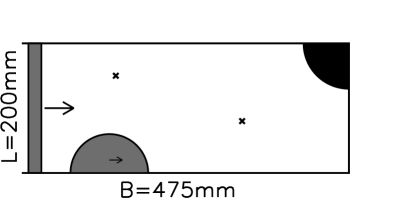
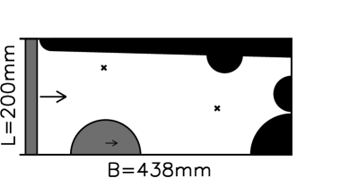
Figure 4: Geometry of the billiards (figure taken from Schäfer et al. (2005)). In the billiard in the right figure bouncing ball orbits have been avoided by inserting additional elements.

The dynamics of classical electromagnetic waves in a thin resonator is equivalent to the Schrödinger equation of a single quantum particle with two degrees of freedom. This is exploited in the microwave cavity experiments, where properties of two dimensional quantum billiards can be studied. The Marburg group considered cavities (Fig. 4) consisting of a rectangle with inserts that assure chaotic, but not necessarily hyperbolic, ray behavior. Both situations, with and without parabolic manifolds leading to so-called bouncing ball states, were considered. The presence of bouncing ball states is known to lead to a weak deviation from RMT behavior Alt et al. (1995). This will serve to check how important small deviation, from the “universal” RMT behaviour, can be for fidelity decay. One of the walls was movable in small steps allowing the perturbation $V$ occurring in an echo experiment [see eq. (12)]. It is important to note that the shift of the wall changes the mean level density and by consequence the Heisenberg time. This trivial perturbation, which would cause very rapid fidelity decay, is eliminated in this case by measuring all times in proper dimensionless units, i.e. in terms of the Heisenberg time. Two antennae allow to measure both reflection and transmission channels. The experiment was carried out in the frequency domain. Afterwards the Fourier transform is used to obtain correlation functions in the time domain. We thus get autocorrelation functions for any given configuration, as well as cross correlation functions associated with the different positions of the moving wall, i.e. between evolutions with different Hamiltonians. After normalizing the latter with the autocorrelation we find the so called scattering fidelity. For chaotic systems, in the weak perturbation limit, scattering fidelity has been shown to be equivalent to the fidelity amplitude Schäfer et al. (2005). Figure 5 shows the experimental and theoretical result in excellent agreement in the absence of bouncing ball states and, as expected, in lesser agreement if they are present. In principle in our model the perturbation strength $\epsilon$ is a free parameter. Yet in this case it was obtained independently by exploring the level-dynamics, i.e. the movement of the energy levels under change of the Hamiltonian. The same random matrix model can account for this situation. For low frequency ranges where resonances are well separated, this so-called level dynamics can be measured. The perturbation strength was extracted and used in the formula for fidelity decay.

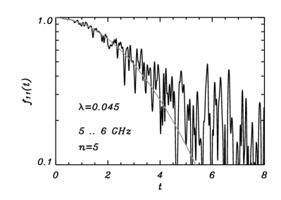
Figure 5: Logarithmic plot of the scattering fidelity $f_{11}(t)$, directly related to the fidelity amplitudes (figure taken from Schäfer et al. (2005)). The smooth curve shows the linear-response result. For the billiard without bouncing balls, the perturbation parameter $\epsilon$ was obtained from the variance of the level velocities; in the other case it was fitted to the experimental curve.

Similar experiments have been performed by Weaver and Lobkis Lobkis and Weaver (2003) on the coda of vibrations of metal blocks. Using the concept of scattering fidelity, these experiments can be reinterpreted as fidelity measurements Gorin et al. (2006a). Quantum optics techniques in principle allow direct measurement of the fidelity amplitude, using a single qubit as a probe. The general context in which this is possible is shown in Gorin et al. (2004c) and a detailed proposal for the experiment is given in Haug et al. (2005) for the case of a kicked rotor where the kicking strength is perturbed. Actual experiments where not performed yet, though an experiment with four different Hamiltonians, two for the forward and two for the backward evolution was performed Andersen et al. (2003).

3.5 Residual perturbations and the Quantum freeze

After the Heisenberg time, fidelity decay is essentially Gaussian, if it has not yet decayed significantly [see eq. (27)]. This decay is determined by the diagonal elements of the perturbation (in the interaction picture) in the eigenbasis of $H_{0}$. If this term is zero or very small, we should see a considerable slowing down of fidelity decay. That such a possibility exists was first noted for particular integrable Prosen and Žnidarič (2003) and chaotic Prosen and Žnidarič (2005) dynamical systems. Yet the generality of the phenomenon is best understood in the context of the RMT model discussed in Gorin et al. (2006b, c).

Sticking to the representation where $H_{0}$ is diagonal, we shall thus consider situations where the perturbation is some random matrix with zero diagonal. The off diagonal elements will form the so called residual interaction $V_{\rm res}=V$. Many ways to implement such a residual perturbation are conceivable. Most are basis dependent. The case, where $H_{0}$ is chosen from a GOE and $V$ is an antisymmetric Hermitian random Gaussian matrix is of interest, because the real matrix $H_{0}$ can be diagonalized without disturbing the residual (i.e. zero diagonal) character of the perturbation. Thus it has strong invariance properties and indeed this case is the only random matrix model, so far, for which an exact analytical result has been obtained Gorin et al. (2006c); Stöckmann and Kohler (2006) by supersymmetric techniques.

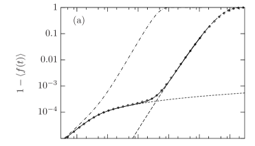
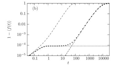
Figure 6: The complement of the average fidelity amplitude $1-\langle f(t)\rangle$, for a weak perturbation, $\epsilon=5\times 10^{-5}$. Frame (a) shows the GOE case with a purely imaginary antisymmetric random Gaussian perturbation. Frame (b) shows the GUE case, with an independent GUE with deleted diagonal as perturbation. The exponentiated linear response approximations are plotted with short dashed lines (for comparison, the exact results for full GOE and GUE perturbations are shown with chain curves). The forth order results Schäfer et al. (2005) from time-independent perturbation theory are plotted with long dashed lines. In the GOE case, the exact analytical result is plotted with a solid line. The random matrix simulations are plotted with points. (Taken from Gorin et al. (2006c).)

Consider the case of a random perturbation (of GUE or GOE type) with diagonal elements set to zero. We have a clearcut stabilization of fidelity after the Heisenberg time because the double integral in the linear response expression cancels the linear term in $t$ exactly for the GUE case and (up to a logarithmic correction) the GOE case. As mentioned, above the quadratic term is absent, and decay, as obtained by linear response, essentially ends at the Heisenberg time. Decay at much larger times results from the next term in the Born series and will go as $\epsilon^{4}$.

We see in Figure 6 that Monte Carlo calculations agree perfectly with the exact solution for the GOE case with antisymmetric perturbation. Furthermore both the GOE and the GUE cases are well described by the linear response result up to the plateau and the end of the plateau agrees with the behavior of $\epsilon^{4}$ term. Experiments are not available yet, but good agreement was shown with a dynamical model Gorin et al. (2006b, c).

The case with zeros forced on the diagonal of the perturbation is not as artificial as it might seem, because is is a standard practice of mean field theory to include the diagonal part of the residual interaction, which does not affect eigenfunctions, in the zero order mean field Hamiltonian. This leaves the residual interaction with zero diagonal. Unfortunately, in such a situation, even if the single particle spectrum is of RMT type, the spectrum of the $n$-particle problem without residual interaction looks more like a random spectrum, and this gets worth if the diagonal term of the interaction is included in $H_{0}$. In such a case the linear term after Heisenberg time is not canceled, and we find linear decay after Heisenberg time Gorin et al. (2006b). In Pižorn et al. (2007) fidelity decay of two-body random ensembles for $n$ Fermions were studied including the diagonal part of the two-body interaction in $H_{0}$. The linear decay for the average fidelity decay was found. Yet remarkably it was shown, that the median behavior does display the freeze. This means, that in a typical realization the freeze is present and thus the time evolution of a mean field theory with weak residual interaction will follow the exact one, after some initial deviation, for a long time.

4 Purity

We now turn our attention to the second problem addressed in the introduction. We shall study the loss of coherence due to coupling to, and entanglement with, some outer system. This is what people often refer to as decoherence. Quantifying and eventually controlling the degree of decoherence is a mayor problem of quantum information. Assuming a pure state in a bipartite system $\mathcal{H}=\mathcal{H}_{A}\otimes\mathcal{H}_{B}$, one can quantify the degree of entanglement via the purity. Let $|\psi\rangle\in\mathcal{H}$ be the pure state in the whole Hilbert space. The reduced density matrix of system $A$ ($B$) is then $\rho_{A}=\mathop{\mathrm{tr}}\nolimits_{B}|\psi\rangle\langle\psi|$ ($\rho_{B}=\mathop{\mathrm{tr}}\nolimits_{A}|\psi\rangle\langle\psi|$). Purity is simply

$$P=\mathop{\mathrm{tr}}\nolimits\rho_{A}^{2}=\mathop{\mathrm{tr}}\nolimits\rho_{B}^{2}$$ (31)

which measures the degree of mixedness of each reduced density matrix. One could also use other mixedness measures such as the von Neumann entropy. We prefer purity above others because it has an analytic structure that simplifies analytic treatment. In particular it is not necessary to diagonalize the density matrix to obtain purity.

In this section we discuss purity decay, thus quantifying decoherence. First we derive a general expression for purity decay of $n$ non interacting qubits. We shall obtain a sum rule where each term involves a single qubit and its entanglement with the remaining ones Gorin et al. (2007). After that, we assume random matrix environments and couplings, following the scheme proposed in Gorin et al. (2004a); Pineda and Seligman (2007) and developed in detail in Pineda et al. (2007). We shall not develop the model with full generality to keep the discussion at a basic level, allowing us to go slowly through the simplest (though representative) cases.

4.1 $n$ qubit purity decay

First we derive a general formula for purity decay of $n$ qubits under very general assumptions. The problem is solved using the enlarged Hilbert space

$$\mathcal{H}=\mathcal{H}_{\mathrm{e}}\otimes\mathcal{H}_{\mathrm{c}}$$ (32)

where $\mathcal{H}_{\mathrm{c}}$ is the Hilbert space of the central system and $\mathcal{H}_{\mathrm{e}}$ (with dimension $N_{\mathrm{e}}$) is the Hilbert space of the environment. The central system itself has a structure as it is composed of several qubits: $\mathcal{H}_{\mathrm{c}}=\bigotimes_{i=1}^{n}\mathcal{H}_{i}$ with $\dim\mathcal{H}_{i}=2$. The Hamiltonian governing the system has the usual structure

$$H_{\lambda}=H_{\mathrm{c}}+H_{\mathrm{e}}+\lambda V,$$ (33)

where $H_{\mathrm{c}}$ acts on the central system, $H_{\mathrm{e}}$ on the environment and $\lambda V$ is the coupling between central system and environment. We shall moreover require that the Hamiltonian of the central system is local, i.e. $H_{\mathrm{c}}=\sum_{i=1}^{n}H_{i}$ where $H_{i}$ acts on $\mathcal{H}_{i}$. We further require that each qubit is separately coupled to the environment:

$$\lambda V=\sum_{i=1}^{n}\lambda_{i}V^{(i)}$$ (34)

with $V^{(i)}$ acting on $\mathcal{H}_{\mathrm{e}}\otimes\mathcal{H}_{i}$. We do not restrict any component of the Hamiltonian to be time independent, though we shall not explicitly show the time orderings required if such dependence exists.

The state in the whole Hilbert space after a time $t$ is $|\psi(t)\rangle=U_{\lambda}(t)|\psi_{0}\rangle$. $U_{\lambda}(t)$ is the evolution operator at time $t$ associated with the Hamiltonian (33) and $|\psi_{0}\rangle=|\psi_{\mathrm{c}}\rangle\otimes|\psi_{\mathrm{e}}\rangle$ ($|\psi_{\mathrm{c}}\rangle\in\mathcal{H}_{\mathrm{c}}$, $|\psi_{\mathrm{e}}\rangle\in\mathcal{H}_{\mathrm{e}}$) is a separable pure initial state. We write this state as $|\psi_{0}\rangle=\sum_{\mu}x_{\mu}|\mu\rangle$ or, using tensor notation, $|\psi_{0}\rangle=\sum_{i,j,k}x_{ijk}|ijk\rangle$ with $|ijk\rangle$ being an element of an orthonormal separable basis in $\mathcal{H}=\mathcal{H}_{\mathrm{e}}\otimes\mathcal{H}_{\mathrm{q}}\otimes\mathcal{H}_{\mathrm{s}}$. We shall keep the convention that Greek indices are used in the whole Hilbert space whereas Latin ones are used for subsystems.

Purity is the trace of the square of the density matrix of the system in question [eq. (31)]. Thus, we are interested in calculating

$$P(t)=\mathop{\mathrm{tr}}\nolimits_{\mathrm{c}}\left(\mathop{\mathrm{tr}}\nolimits_{\mathrm{e}}|\psi(t)\rangle\langle\psi(t)|\right)^{2}=\mathop{\mathrm{tr}}\nolimits_{\mathrm{c}}\left[\mathop{\mathrm{tr}}\nolimits_{\mathrm{e}}M_{\lambda}(t)|\psi_{0}\rangle\langle\psi_{0}|M^{\dagger}_{\lambda}(t)\right]^{2}$$ (35)

where $M_{\lambda}(t)$ is the echo operator defined in conjunction with fidelity, see section 3. The last equality is obtained noticing that the difference between the forward evolution operator $U_{\lambda}(t)$ and the echo operator $M_{\lambda}(t)$ is the local (with respect to environment-central system separation) operation $U_{0}^{\dagger}(t)$. Since entanglement properties remain unchanged under local operations, purity has the same value for the state evolved with either the forward or the echo evolution operator. Since for large purities $M_{\lambda}(t)\approx\leavevmode\hbox{\small 1\kern-3.8pt\normalsize 1}$, a series expansion is again feasible for long times. We obtain

$$P(t)=1-2\lambda^{2}\int_{0}^{t}\mathrm{d}\tau\int_{0}^{t}\mathrm{d}\tau^{\prime}\mathop{\mathrm{Re}}\nolimits A(\tau,\tau^{\prime})+\mathord{\mathrm{O}}\left(\lambda^{4}\right),$$ (36)

where $A(\tau,\tau^{\prime})=A_{J}(\tau,\tau^{\prime})-A_{1}(\tau,\tau^{\prime})+A_{2}(\tau,\tau^{\prime})-A_{3}(\tau,\tau^{\prime})$ and

$$A_{J}(\tau,\tau^{\prime}) =p[\tilde{V}_{\tau}\tilde{V}_{\tau^{\prime}}\varrho_{0}\otimes\varrho_{0}]=x_{\mu}x_{i^{\prime}jk}^{*}x_{i^{\prime}j^{\prime}k^{\prime}}x_{ij^{\prime}k^{\prime}}^{*}[\tilde{V}_{\tau}\tilde{V}_{\tau^{\prime}}]_{ijk,\mu},$$ (37a)

$$A_{2}(\tau,\tau^{\prime}) =p[\tilde{V}_{\tau^{\prime}}\varrho_{0}\tilde{V}_{\tau}\otimes\varrho_{0}]=x_{\mu}x_{\nu}^{*}x_{i^{\prime}j^{\prime}k^{\prime}}x_{ij^{\prime}k^{\prime}}^{*}[\tilde{V}_{\tau}]_{ijk,\mu}[\tilde{V}_{\tau^{\prime}}]_{i^{\prime}jk,\nu}^{*},$$ (37b)

$$A_{3}(\tau,\tau^{\prime}) =p[\tilde{V}_{\tau^{\prime}}\varrho_{0}\otimes\varrho_{0}\tilde{V}_{\tau}]=x_{\mu}x_{i^{\prime}jk}^{*}x_{i^{\prime}j^{\prime}k^{\prime}}x_{\nu}^{*}[\tilde{V}_{\tau}]_{ijk,\mu}[\tilde{V}_{\tau^{\prime}}]_{ij^{\prime}k^{\prime},\nu}^{*}$$ (37c)

(summation over repeated indices is assumed in these equations). The bilinear functional $p[\rho_{1}\otimes\rho_{2}]=\mathop{\mathrm{tr}}\nolimits(\mathop{\mathrm{tr}}\nolimits_{\mathrm{e}}\rho_{1}\mathop{\mathrm{tr}}\nolimits_{\mathrm{e}}\rho_{2})$ has been introduced, together with $\rho_{0}=|\psi_{0}\rangle\langle\psi_{0}|$, to simplify the expressions. Notice that each term depends on the coupling in the interaction picture, see eq. (15).

Taking advantage of the particular structure of the coupling [eq. (34)] we can rewrite the integrand in eq. (36) as a sum of terms, each with two indices labeling the qubits.

$$\lambda^{2}A(\tau,\tau^{\prime})=\sum_{i,j=1}^{n}\lambda_{i}\lambda_{j}A^{(i,j)}(\tau,\tau^{\prime})$$

with

$$A^{(i,j)}(\tau,\tau^{\prime})=p[\tilde{V}^{(i)}_{\tau}\tilde{V}^{(j)}_{\tau^{\prime}}\varrho_{0}\otimes\varrho_{0}]-p[\tilde{V}^{(i)}_{\tau^{\prime}}\varrho_{0}\tilde{V}^{(j)}_{\tau}\otimes\varrho_{i}]\\ +p[\tilde{V}^{(i)}_{\tau}\varrho_{0}\otimes\tilde{V}^{(j)}_{\tau^{\prime}}\varrho_{0}]-p[\tilde{V}^{(i)}_{\tau^{\prime}}\varrho_{0}\otimes\varrho_{0}\tilde{V}^{(j)}_{\tau}]\;.$$ (38)

The terms $A^{(i,j)}(\tau,\tau^{\prime})$ are cross correlation functions for $i\neq j$ and autocorrelation functions for $i=j$. If the cross correlation functions drop to zero fast enough, these terms can be neglected. This happens if the environment Hamiltonian is chaotic Gorin et al. (2007) or if the couplings are independent from the outset. Assuming fast decay of cross correlation functions [$A^{(i\neq j,j)}\approx 0$] we obtain

$$P(t) =1-\sum_{i=1}^{n}\left(1-P^{(i)}_{\rm sp}(t)\right),$$ (39)

$$P^{(i)}_{\rm sp}(t) =1-2\lambda_{i}^{2}\int_{0}^{t}\mathrm{d}\tau\int_{0}^{t}\mathrm{d}\tau^{\prime}A^{(i,i)}(\tau,\tau^{\prime})+\mathord{\mathrm{O}}\left(\lambda_{i}^{4}\right).$$

Each term $P^{(i)}_{\rm sp}(t)$ represents purity decay of the whole register when only a single qubit is coupled to the environment. That configuration is called spectator configuration. Eq. (39) is a sum rule for decoherence and is the central result of Gorin et al. (2007).

4.2 RMT in the spectator configuration

We now solve the problem of a single qubit in the spectator configuration, when the Hamiltonian of the environment and the coupling are chosen from the classical ensembles. We use the following subscripts: “c” (for central system), “e” (for environment) , “q” (for the coupled qubit), and “s” (for the spectator).

We have seen that the problem can be formulated in terms of the echo operator. However, in the spectator configuration, the echo operator does not contain the internal Hamiltonian of the spectator space. Effectively one can thus drop those terms and write $H_{0}=H_{\mathrm{e}}+H_{\mathrm{q}}$ (with $H_{\mathrm{q}}$ the internal Hamiltonian of the coupled qubit) and $H_{\lambda}=H_{0}+\lambda V$ with $\lambda V$ the coupling between the coupled qubit and the environment. Notice how no part of the Hamiltonian is acting on the spectator space.

At this point we rederive a result from Pineda et al. (2007). Purity decay in the spectator configuration depends only on $\rho_{\mathrm{q}}=\mathop{\mathrm{tr}}\nolimits_{\mathrm{s}}|\psi_{\mathrm{c}}\rangle\langle\psi_{\mathrm{c}}|$ the reduced density matrix of the coupled qubit alone:

$$P(t) =\mathop{\mathrm{tr}}\nolimits_{\mathrm{c}}\left[\mathop{\mathrm{tr}}\nolimits_{\mathrm{e}}M_{\lambda}\otimes\leavevmode\hbox{\small 1\kern-3.8pt\normalsize 1}_{\mathrm{s}}|\psi_{0}\rangle\langle\psi_{0}|M_{\lambda}^{\dagger}\otimes\leavevmode\hbox{\small 1\kern-3.8pt\normalsize 1}_{\mathrm{s}}\right]^{2}$$ (40)

$$=\mathop{\mathrm{tr}}\nolimits_{\mathrm{e}}\left[\mathop{\mathrm{tr}}\nolimits_{\mathrm{c}}M_{\lambda}\otimes\leavevmode\hbox{\small 1\kern-3.8pt\normalsize 1}_{\mathrm{s}}|\psi_{0}\rangle\langle\psi_{0}|M_{\lambda}^{\dagger}\otimes\leavevmode\hbox{\small 1\kern-3.8pt\normalsize 1}_{\mathrm{s}}\right]^{2}$$ (41)

$$=\mathop{\mathrm{tr}}\nolimits_{\mathrm{e}}\left[\mathop{\mathrm{tr}}\nolimits_{\mathrm{q}}M_{\lambda}(\mathop{\mathrm{tr}}\nolimits_{\mathrm{s}}|\psi_{0}\rangle\langle\psi_{0}|)M_{\lambda}^{\dagger}\right]^{2}$$ (42)

$$=\mathop{\mathrm{tr}}\nolimits_{\mathrm{e}}\left[\mathop{\mathrm{tr}}\nolimits_{\mathrm{q}}M_{\lambda}(\rho_{\mathrm{q}}\otimes|\psi_{\mathrm{e}}\rangle\langle\psi_{\mathrm{e}}|)M_{\lambda}^{\dagger}\right]^{2}.$$ (43)

The first step uses only that the dynamics in the spectator space is trivial. In the second step we use the property that for a pure bipartite system, purity does not depend on the subsystem observed. Thus instead of measuring purity of the quantum register we formally calculate purity of the environment. In the next step we split the trace over all the register into the trace over the coupled qubit and the trace over the spectator qubits. Next, we explicitly shift the trace over the spectator space to one over the initial state obtaining the final result: purity decay in the spectator configuration will only depend on the reduced density matrix of the coupled qubit.

Since to purify a qubit we only need one additional qubit, we can replace $\mathcal{H}_{\mathrm{s}}$ by the Hilbert space of a single qubit thus greatly reducing the complexity of the problem! We can now refer to the solution published in Pineda et al. (2007) for two qubits without loosing generality. We carry on the explicit calculations, in a simple case.

We assume that the nontrivial part of $V$ is well described by the GUE, with a normalization set by the condition

$$\langle V_{ij,kl}\rangle=0,\quad\langle V_{ij,kl}V_{i^{\prime}j^{\prime},k^{\prime}l^{\prime}}\rangle=(\delta_{j,l}\delta_{j^{\prime},l^{\prime}})(\delta_{i,k^{\prime}}\delta_{i^{\prime},k})$$ (44)

where the $i$s and $k$s run over the environment and the coupled qubit whereas the $i$s and $j$s run over the spectator qubit. The first set of $\delta$s describe the fact that the spectator is not coupled, and the second set of $\delta$s is the usual GUE relation. The normalization condition is no restriction as an arbitrary factor can be absorbed in the coupling constant $\lambda$. However this normalization guarantees that decoherence decay is roughly independent on the environment size, for big environments. One could also assume that $V$ is well described by the GOE, however this leads to complications (due to the weaker invariance properties of the ensemble) on which we do not want to dwell Kaplan et al. (2007). We first average over the coupling. To do so we chose a basis that diagonalizes $H_{0}$. In this basis, $[\tilde{V}_{\tau}]_{ij,i^{\prime}j^{\prime}}=\delta_{j,j^{\prime}}\mathrm{e}^{\mathrm{i}tE_{i}}V_{i,i^{\prime}}\mathrm{e}^{-\mathrm{i}tE_{i^{\prime}}}$. The $i$s and $j$s run over $\mathcal{H}_{\mathrm{e}}\otimes\mathcal{H}_{\mathrm{q}}$ and $\mathcal{H}_{\mathrm{s}}$ respectively, and both $E_{i}$ and $E_{i^{\prime}}$ are eigenenergies of $H_{0}$. As long as $V$ and $H_{0}$ are independent, relations (44) remain unchanged, so we can write

$$\langle[\tilde{V}_{\tau}\tilde{V}_{\tau^{\prime}}]_{ij,i^{\prime}j^{\prime}}\rangle=\sum_{i^{\prime\prime}=1}^{2N_{\mathrm{e}}}\sum_{j^{\prime\prime}=1}^{2}\mathrm{e}^{\mathrm{i}\tau(E_{i}-E_{i^{\prime\prime}})+\mathrm{i}\tau^{\prime}(E_{i^{\prime\prime}}-E_{i^{\prime}})}\langle V_{ij,i^{\prime\prime}j^{\prime\prime}}V_{i^{\prime\prime}j^{\prime\prime},i^{\prime}j^{\prime}}\rangle=\delta_{ij,i^{\prime}j^{\prime}}\sum_{i^{\prime\prime}}\mathrm{e}^{\mathrm{i}(\tau-\tau^{\prime})(E_{i}-E_{i^{\prime}})}\\$$ (45)

and

$$\langle[\tilde{V}_{\tau}]_{ij,kl}[\tilde{V}_{\tau^{\prime}}]_{i^{\prime}j^{\prime},k^{\prime}l^{\prime}}\rangle=\langle[\tilde{V}_{\tau}]_{ij,kl}[\tilde{V}_{\tau^{\prime}}]_{k^{\prime}l^{\prime},i^{\prime}j^{\prime}}^{*}\rangle=\\ \mathrm{e}^{\mathrm{i}\tau(E_{i}-E_{k})+\mathrm{i}\tau^{\prime}(E_{i^{\prime}}-E_{k^{\prime}})}\langle V_{ij,kl}V_{i^{\prime}j^{\prime},k^{\prime}l^{\prime}}\rangle=\delta_{ij,k^{\prime}l}\delta_{kj^{\prime},i^{\prime}l^{\prime}}\mathrm{e}^{\mathrm{i}(\tau-\tau^{\prime})(E_{i}-E_{k})}.$$ (46)

This greatly simplifies eqs. (37).

A further step towards obtaining the final expression is to average over the state of the environment. In order to ease the following work, we rewrite the separability condition as $x_{ijk}=\psi_{i}\phi_{jk}$ where $|\psi_{\mathrm{c}}\rangle=\sum_{i}\psi_{i}|i\rangle$ is the initial state of the environment and $|\psi_{\mathrm{c}}\rangle=\sum_{j,k}\phi_{jk}|jk\rangle$ the state of the two qubits. However, we wish to write $|\psi_{\mathrm{c}}\rangle$ in its simplest form. We use the invariance properties of the ensemble defined by $H_{\lambda}$, but under the restriction that $H_{0}$ is still diagonal [to be able to write eqs. (45) and (46)]. This freedom allows any unitary operation on the purifying qubit, and a phase transformation $\exp(\mathrm{i}\alpha H_{\mathrm{q}})$ of the eigenvectors of $H_{\mathrm{q}}$ ($\alpha\in\mathbb{R}$). Taking into account this freedom we now show how to construct a basis $\{|0\rangle,|1\rangle\}\otimes\{|0\rangle,|1\rangle\}$ in which an arbitrary initial state of the central system can be written as

$$|\psi_{\mathrm{c}}\rangle=\cos\theta_{1}(\cos\theta_{2}|0\rangle+\sin\theta_{2}|1\rangle)|0\rangle+\sin\theta_{1}(\sin\theta_{2}|0\rangle-\cos\theta_{2}|1\rangle)|1\rangle,$$ (47)

and still, $H_{\mathrm{q}}=\frac{\Delta}{2}|0\rangle\langle 0|-\frac{\Delta}{2}|1\rangle\langle 1|$ is diagonal. To find this basis we start using the Schmidt decomposition to write

$$|\psi_{\mathrm{c}}\rangle=\cos\theta_{1}|\tilde{0}_{1}\tilde{0}_{2}\rangle+\sin\theta_{1}|\tilde{1}_{1}\tilde{1}_{2}\rangle$$ (48)

with $\{|\tilde{0}_{i}\rangle,|\tilde{1}_{i}\rangle\}$ being an orthonormal basis of particle $i$. For the coupled qubit, we fix the $z$ axis of the Bloch sphere (containing both $|0\rangle$ and $|1\rangle$) parallel to the eigenvectors of $H_{\mathrm{q}}$, and the $y$ axis perpendicular (in the Bloch sphere) to both the $z$ axis and $|\tilde{0}_{1}\rangle$. The states contained in the $xz$ plane are then real superpositions of $|0\rangle$ and $|1\rangle$, which implies that $|\tilde{0}_{1}\rangle=\cos\theta_{2}|0\rangle+\sin\theta_{2}|1\rangle$ and $|\tilde{1}_{1}\rangle=\sin\theta_{2}|0\rangle-\cos\theta_{2}|1\rangle$ for some $\theta_{2}$. In the second qubit it is enough to set $|0\rangle=|\tilde{0}_{2}\rangle$ and $|1\rangle=|\tilde{1}_{2}\rangle$. This freedom is also related to the fact that purity only depends on $\rho_{\mathrm{q}}=\mathop{\mathrm{tr}}\nolimits_{\mathrm{s}}|\psi_{\mathrm{c}}\rangle\langle\psi_{\mathrm{c}}|$. A visualization of this procedure is found in fig. 7. The angle $\theta_{1}\in[0,\pi/4]$ measures the entanglement between the coupled qubit and the spectator space whereas the angle $\theta_{2}\in[0,\pi/2]$ is related to an initial magnetization of the coupled qubit.

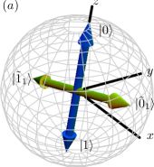
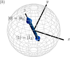
Figure 7: (Color online) We present a plot to help visualize the way the initial condition is parametrized. On the left, the coupled qubit. The eigenvectors of its internal Hamiltonian ($|0\rangle$ and $|1\rangle$) are represented in blue. The $z$ axis is chosen parallel to the vector $|0\rangle$. The $x$ axis is chosen in such a way as to make both $|\tilde{0}_{1}\rangle$ and $|\tilde{1}_{1}\rangle$ have real coefficients i.e. such that the $xz$ plane contains $|\tilde{0}_{1}\rangle$ and $|\tilde{1}_{1}\rangle$. On the right we represent the second qubit where we have absolute freedom to choose the basis (even if an internal Hamiltonian is present), and thus we choose it according to the natural Schmidt decomposition.

We have then that

$$\mathop{\mathrm{Re}}\nolimits\langle A_{J}\rangle =\mathop{\mathrm{Re}}\nolimits\sum_{i,i^{\prime}=1}^{N_{\mathrm{e}}}\sum_{j,j^{\prime},k,k^{\prime}=0}^{1}|\psi_{i}|^{2}|\psi_{i^{\prime}}|^{2}|\phi_{jk}|^{2}|\phi_{j^{\prime}k^{\prime}}|^{2}\sum_{i^{\prime\prime}=1,j^{\prime\prime}=0}^{N_{\mathrm{e}},1}\mathrm{e}^{\mathrm{i}(\tau-\tau^{\prime})(E_{ij}-E_{i^{\prime\prime}j^{\prime\prime}})}$$

$$\approx\mathop{\mathrm{Re}}\nolimits\sum_{i}\left(|\psi_{i}|^{2}\sum_{i^{\prime\prime}}\mathrm{e}^{\mathrm{i}(\tau-\tau^{\prime})(E_{i}-E_{i^{\prime\prime}})}\right)\mathop{\mathrm{Re}}\nolimits\sum_{jk}\left(|\phi_{jk}|^{2}\sum_{j^{\prime\prime}}\mathrm{e}^{\mathrm{i}(\tau-\tau^{\prime})(E_{j}-E_{j^{\prime\prime}})}\right)$$

$$\approx\frac{1}{N_{\mathrm{e}}}\left(\mathop{\mathrm{Re}}\nolimits\sum_{i,i^{\prime\prime}}\mathrm{e}^{\mathrm{i}(\tau-\tau^{\prime})(E_{i}-E_{i^{\prime\prime}})}\right)\left(\sum_{jk}|\phi_{jk}|^{2}\mathop{\mathrm{Re}}\nolimits\mathrm{e}^{\mathrm{i}(\tau-\tau^{\prime})E_{j}}\right)\left(\sum_{j^{\prime\prime}}\mathrm{e}^{\mathrm{i}(\tau-\tau^{\prime})E_{j^{\prime\prime}}}\right)$$

$$=2\cos^{2}\left[\frac{(\tau-\tau^{\prime})\Delta}{2}\right]\mathop{\mathrm{Re}}\nolimits K_{2}(\tau-\tau^{\prime})$$ (49)

$$=\mathop{\mathrm{Re}}\nolimits K_{2}(\tau-\tau^{\prime})\left[1+\cos(\Delta(\tau-\tau^{\prime})\right]$$ (50)

Several approximations have been done. In the first step we assume that the imaginary contribution from the environment is very small. This is justified noticing that the form factor of a random matrix ensemble is real [eq. (7)]. We also take into account the normalization condition of the states. In the second step we consider that all eigenstates contribute similarly and replace each $|\psi_{i}|^{2}$ by its average value $1/N_{\mathrm{e}}$. We end up with an simple expression in the qubit (independent of the initial condition) and the form factor [eq. (7)] of the environment. We are also assuming that the level separation in $H_{\mathrm{q}}$ is $\Delta$ so $E_{0}=-E_{1}=\Delta/2$.

Studying the average over initial conditions in the environment leads to the observation that $\langle A_{1}\rangle=\langle A_{2}\rangle=\mathord{\mathrm{O}}(1/N_{\mathrm{e}})$. The remaining term can be computed along the same lines (i.e. same techniques and assumptions), however its calculation is both cumbersome and boring. We leave it to the enthusiastic student. Its result is

$$\mathop{\mathrm{Re}}\nolimits\langle A_{3}\rangle=\mathop{\mathrm{Re}}\nolimits K_{2}(\tau-\tau^{\prime})\left\{1-g_{1}(\theta_{1},\theta_{2})+\left[1-g_{2}(\theta_{1},\theta_{2})\right]\cos[\Delta(\tau-\tau^{\prime})]\right\}$$ (51)

where $g_{1}(\theta_{1},\theta_{2})$ and $g_{2}(\theta_{1},\theta_{2})$ are geometric factors that depend on the initial state. Their values are given by

$$g_{1}({\theta_{1},\theta_{2}}) =g(\theta_{1})[1-g(\theta_{2})]+g(\theta_{2})[1-g(\theta_{1})]$$ (52)

$$g_{2}({\theta_{1},\theta_{2}}) =2[1-g(\theta_{1})]-g(\theta_{2})[1-2g(\theta_{1})],$$ (53)

where $g(\theta)=\cos^{4}\theta+\sin^{4}\theta$.

The general solution for purity using this parametrization is

$$P(t)=1-2\lambda^{2}\int_{0}^{t}\mathrm{d}\tau\int_{0}^{\tau}\mathrm{d}\tau^{\prime}[1+\delta(\tau^{\prime}/\tau_{\mathrm{H}})-b_{2}(\tau^{\prime}/\tau_{\mathrm{H}})]\\ \times\big{[}g_{1}(\theta_{1},\theta_{2})+g_{2}(\theta_{1},\theta_{2})\cos\Delta\tau^{\prime}\big{]}+\mathord{\mathrm{O}}(\lambda^{4}).$$ (54)

Two meaningful limits can be studied, the degenerate limit, in which the spacing of the internal Hamiltonian is much smaller than the inverse of the Heisenberg time of the environment ($\Delta\ll 1/\tau_{\mathrm{H}}$), and the fast limit ($\Delta\gg 1/\tau_{\mathrm{H}}$) in which the opposite condition is met. In the degenerate limit purity decay is given by

$$P_{\rm D}(t)=1-\lambda^{2}(2-g_{\theta_{1}})r(t),$$ (55)

where

$$r(t)=t\max\{t,\tau_{\mathrm{H}}\}+\frac{2}{3\tau_{\mathrm{H}}}\min\{t,\tau_{\mathrm{H}}\}^{3}.$$ (56)

The result is independent of $\theta_{2}$ since a degenerate Hamiltonian is, in this context, equivalent to no Hamiltonian at all. The $\theta_{1}$-dependence in this formula shows that an entangled qubit pair is more susceptible to decoherence than a separable one. In the fast limit we obtain

$$P_{\rm F}(t)=1-\lambda^{2}\left[g_{1}(\theta_{1},\theta_{2})r(t)+2\tau_{\mathrm{H}}g_{2}(\theta_{1},\theta_{2})t\right].$$ (57)

For initial states chosen as eigenstates of $H_{\mathrm{q}}$ we find linear decay of purity both below and above Heisenberg time. In order for $\rho_{\mathrm{q}}$ to be an eigenstate of $H_{\mathrm{q}}$ it must, first of all, be a pure state (in $\mathcal{H}_{\mathrm{q}}$). Therefore this behavior can only occur if $\theta_{1}=0$ or $\theta_{1}=\pi/2$. Apart from that particular case, we observe in both limits, the fast as well as the degenerate limit, the characteristic linear/quadratic behavior before/after the Heisenberg time similar to the behavior of fidelity decay.

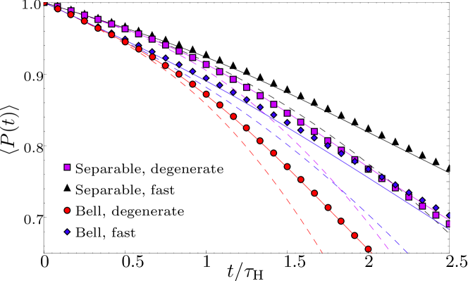
Figure 8: (Color online) Numerical simulations for the average purity as a function of time in units of the Heisenberg time of the environment (spectator configuration, GUE case). For the coupling strength $\lambda=0.03$ we show the dependence of $\langle P(t)\rangle$ on the level splitting $\Delta$ in $H_{1}$ and on the initial degree of entanglement between the two qubits (in all cases $\theta_{2}=\pi/4$): $\theta_{1}=0$ (separable states), $\Delta=8$ (black triangles); $\theta_{1}=\pi/4$ (Bell states), $\Delta=8$ (blue rhombus); $\theta_{1}=0$, $\Delta=0$ (purple squares); $\theta_{1}=\pi/4$, $\Delta=0$ (red circles). We also show the corresponding linear response results (dashed lines) and exponentiated linear response results (solid lines). They are plotted with the same color, as the respective numerical data. In all cases $N_{\mathrm{e}}=1024$.

In Fig. 8 we show numerical simulations for the average purity decay. We average over 30 different Hamiltonians each probed with 45 different initial conditions. We contrast Bell states ($\theta_{2}=\pi/4$, $\theta_{1}=\pi/4$) with separable states ($\theta_{2}=\pi/4$, $\theta_{1}=0$), and also systems with a large level splitting ($\Delta=8$) in the first qubit with systems having a degenerate Hamiltonian ($\Delta=0$). The results presented in this figure show that entanglement generally enhances decoherence. This can be anticipated since for fixed $\theta_{2}$, increasing the value of $\theta_{1}$ (and hence entanglement) increases both $g_{1}(\theta_{1},\theta_{2})$ and $g_{2}(\theta_{1},\theta_{2})$. At the same time we find again that increasing $\Delta$ tends to reduce the rate of decoherence, while a strict inequality only holds among the two limiting cases (just as in the one qubit case). From $g_{2}(\theta_{1},\theta_{2})=2-g_{1}(\theta_{1},\theta_{2})-g(\theta_{1})$, it follows that $(P_{\rm F}-P_{\rm D})/\lambda^{2}=g_{2}(\theta_{1},\theta_{2})[r(t)-2t\tau_{\mathrm{H}}]\geq 0$. Therefore, for fixed initial conditions and $t$ greater than 0, $P_{\rm F}(t)>P_{\rm D}(t)$. This is the second aspect illustrated in fig. 8.

The linear response formulae derived throughout this section are expected to work for high purities or, equivalently, when the second order Born expansion of the echo operator is a good approximation; it is of obvious interest to extend them to cover a larger range. The extension of fidelity linear response formulae has, in some cases, been done with some effort using super-symmetry techniques. This has been possible partly due to the simple structure of the fidelity amplitude, but trying to use this approach for a more complicated object such as purity seems to be out of reach for the time being. Exponentiating the formulae obtained from the linear response formalism has proven to be in good agreement with the exact super-symmetric and/or numerical results for fidelity, if the perturbation is not too big. The exponentiation of the linear response formulae for purity can be compared with Monte Carlo simulations in order to prove its validity. We now explain the details required to implement this procedure.

Given a linear response formula $P_{\rm LR}(t)$ for which $P(0)=1$ [like eqs. (54), (55), or (57)], and an expected asymptotic value for infinite time $P_{\infty}$, the exponentiation reads

$$P_{\rm ELR}(t)=P_{\infty}+(1-P_{\infty})\exp\left[-\frac{1-P_{\rm LR}(t)}{1-P_{\infty}}\right].$$ (58)

This particular form guaranties that $P_{\rm ELR}$ equals $P_{\rm LR}$ for short times, and that $\lim_{t\to\infty}P_{\rm ELR}(t)=P_{\infty}$ The particular value of $P_{\infty}$ will depend on the physical situation; in our case it will depend on the configuration and on the initial conditions.

Consider the spectator configuration. Let us write the initial condition as

$$|\psi_{\mathrm{c}}(\theta)\rangle=\cos\theta_{1}|\tilde{0}_{\mathrm{q}}\tilde{0}_{\mathrm{s}}\rangle+\sin\theta_{1}|\tilde{1}_{\mathrm{q}}\tilde{1}_{\mathrm{s}}\rangle$$ (59)

for some rotated basis. We assumed that for long enough times, the totally depolarizing channel $\mathcal{E}_{\rm d}$ will act (recall that the totally depolarizing channel is defined as $\mathcal{E}_{\rm d}[\rho]=\leavevmode\hbox{\small 1\kern-3.8pt\normalsize 1}/\mathop{\mathrm{tr}}\nolimits\leavevmode\hbox{\small 1\kern-3.8pt\normalsize 1}$ for any density matrix $\rho$) on the coupled qubit. Hence, for the spectator configuration, the final value of purity is assumed to be

$$P_{\infty}=P\left(\mathcal{E}_{\rm d}\otimes\leavevmode\hbox{\small 1\kern-3.8pt\normalsize 1}[|\psi_{\mathrm{c}}(\theta)\rangle\langle\psi_{\mathrm{c}}(\theta)|]\right)=\frac{g(\theta_{1})}{2}.$$ (60)

Good agreement is found with Monte Carlo simulations for moderate and strong couplings, see fig 8. For weak coupling $P_{\infty}$ depends on the coupling strength.

4.3 Two qubit concurrence decay

\psfrag{a}{}\psfrag{C}{$C$}\psfrag{P}{$P$}\psfrag{dimHe}{$\dim\mathcal{H}_{\mathrm{e}}$}\psfrag{8}{8}\psfrag{16}{16}\psfrag{32}{32}\psfrag{64}{64}\psfrag{128}{128}\psfrag{256}{256}\includegraphics{ConvergeNoConvergeCPBW}

Figure 9: (Color online) We present the concurrence-purity $CP$ plane. The area allowed for physical states is the gray area plus the set $\{(0,P),P\in[1/4,1/3]\}$. The Werner curve eq. (62) is shown as a thick black solid line. We show curves $(\langle C(t)\rangle,\langle P(t)\rangle)$ as obtained from numerical simulations of the spectator Hamiltonian. We choose $\Delta=1$ and vary $\dim(\mathcal{H}_{\mathrm{e}})$ for two different coupling strengths $\lambda=0.02$ (thick lines) and $\lambda=0.14$ (thin lines). The resulting curves are plotted with different colors, according to $\dim(\mathcal{H}_{\mathrm{e}})$ as indicated in the figure.

In the previous section we studied purity decay of $n$ qubits. Purity measures entanglement with the environment, but we can wonder how decoherence affects the internal quantum mechanical properties of the central system. Possibly the most important quantum mechanical property of a multi-particle system is its internal entanglement. We consider the simples scenario in which it is possible to have entanglement: a two qubit subsystem. Two qubit entanglement can measured with the concurrence $C$, a measure used extensively in the literature Mintert et al. (2005) that is straightforward to calculate. It is closely related to the entanglement of formation, which measures the minimum number of Bell pairs needed to create an ensemble of pure states representing the state to be studied Hill and Wootters (1997). Given a density matrix $\rho$ representing the state of two qubits, concurrence is defined as

$$C(\rho)=\max\{0,\Lambda_{1}-\Lambda_{2}-\Lambda_{3}-\Lambda_{4}\}$$ (61)

where $\Lambda_{i}$ are the eigenvalues of the matrix $\sqrt{\rho(\sigma_{y}\otimes\sigma_{y})\rho^{*}(\sigma_{y}\otimes\sigma_{y})}$ in non-increasing order. The superscript ^∗ denotes complex conjugation in the computational basis and $\sigma_{y}$ is a Pauli matrix Wootters (1998). The concurrence has a maximum value of one for Bell states, and a minimum value of zero for separable states. Furthermore, it is invariant under bi-local unitary operations. However, since concurrence is defined in terms of the eigenvalues of a hermitian $4\times 4$-matrix, an analytical treatment, even in linear response approximation, is much more involved than in the case of purity, and has not been performed.

We shall first explore a relation (first found in Pineda and Seligman (2006), partly explained in Ziman and Buzek (2005), and further studied in Pineda and Seligman (2007); Pineda et al. (2007)) between concurrence and purity. We show that this relation is valid in a wide parameter range. Combining it with the appropriate formula for purity decay, we obtain an analytic prediction for concurrence decay. We compare our prediction with Monte Carlo simulations. It is essential that the two qubits do not interact; otherwise the coupling between the qubits would act as an additional sink (or source) for internal entanglement – a complication we wish to avoid.

\psfrag{q}[cb]{$\log_{2}N_{\mathrm{e}}$}\psfrag{dimHe}[lb]{$N_{\mathrm{e}}$}\psfrag{E}[c]{$\log_{2}D$}\psfrag{a}{(a)}\psfrag{b}{(b)}\psfrag{d}[cb]{$\lambda$}\psfrag{l1}{$\lambda=0.14$}\psfrag{l2}{$\lambda=0.02$}\includegraphics[height=156.49014pt]{onvergeNoConvergeAreaFF_BW}

\psfrag{q}[cb]{$\log_{2}N_{\mathrm{e}}$}\psfrag{dimHe}[lb]{$N_{\mathrm{e}}$}\psfrag{E}[c]{$\log_{2}D$}\psfrag{a}{(a)}\psfrag{b}{(b)}\psfrag{d}[cb]{$\lambda$}\psfrag{l1}{$\lambda=0.14$}\psfrag{l2}{$\lambda=0.02$}\includegraphics[height=156.49014pt]{Error_Vs_DeltaFF_BW}

Figure 10: (Color online) We show $D$ [eq. (63)] which measures a “distance” in the $CP$ plane between numerical curves for the RMT model and the Werner curve. In (a) its dependence on the size of the environment is studied for two cases. For $\lambda=0.02$ a finite value is approached, whereas for $\lambda=0.14$ algebraic decay is seen. The thick line, which is proportional to $N_{\mathrm{e}}^{-1}$, is meant as a guide to the eye. In (b) we plot $D$ as a function of the coupling $\lambda$, for various values of $N_{\mathrm{e}}$. In the large environment limit, and for $\lambda\ll 0.1$, we have a noticeable deviation from the Werner curve. In all cases $\Delta=1$.

We study the relation between concurrence and purity using the $CP$-plane, where we plot concurrence against purity with time as a parameter. This plane is plotted in fig. 9. The gray area indicates the region of physically admissible states Munro et al. (2001). The upper boundary of this region is given by the maximally entangled mixed states. The Werner states $\rho_{\rm W}=\alpha\frac{\leavevmode\hbox{\small 1\kern-3.8pt\normalsize 1}}{4}+(1-\alpha)|\rm{Bell}\rangle\langle\rm{Bell}|$, $0\leq\alpha\leq 1$, define a smooth curve on the $CP$-plane (black solid line). The analytic form of this curve is Pineda and Seligman (2007)

$$C_{\rm W}(P)=\max\left\{0,\frac{\sqrt{12P-3}-1}{2}\right\},$$ (62)

and will be referred to as the Werner curve. However, note that states mapped to the Werner curve are not necessarily Werner states. We perform numerical simulations in the spectator configuration. We compute the average concurrence for a given interval of purity using 15 different Hamiltonians and 15 different initial states for each Hamiltonian. We fix the level splitting in the coupled qubit to $\Delta=1$ and consider two different values $\lambda=0.02$ and $0.14$ for the coupling to the environment. Fig. 9 shows the resulting $CP$-curves for different dimensions of $\mathcal{H}_{\mathrm{e}}$. Observe that for both values of $\lambda$, the curves converge to a certain limiting curve as $\dim(\mathcal{H}_{\mathrm{e}})$ tends to infinity. While for $\lambda=0.02$, this curve is at a finite distance of the Werner curve, for $\lambda=0.14$ it practically coincides with $C_{\rm W}(P)$. Varying the configuration, the coupling strength, the level splitting, or the ensemble (GOE/GUE), gives the same qualitative results in the $CP$ plane, for large dimensions. In some cases we have an accumulation towards the Werner curve, in others there is a small variation.

To study this situation in more detail, consider a $CP$-curve $C_{\rm num}(P)$, obtained from our numerical simulations, and define its “distance” $D$ to the Werner curve as

$$D=\int_{P_{\rm min}}^{1}\mathrm{d}P\left|C_{\rm num}(P)-C_{\rm W}(P)\right|.$$ (63)

The behavior of $D$ as a function of the size of the system is shown in Fig. 10(a). For $\lambda=0.14$ (dark dots), the error goes to zero in an algebraic fashion, at least in the range studied. In fact, from a comparison with the black solid line we may conclude that the deviation $D$ is inversely proportional to the dimension of $\mathcal{H}_{\mathrm{e}}$. By contrast, for $\lambda=0.02$ (light red dots), $D$ tends to a finite value, in line with the assertion that the numerical results converge to a different curve. In Fig. 10(b) we plot the error $D$ as a function of $\lambda$, for different dimensions of $\mathcal{H}_{\mathrm{e}}$. The results suggest an exponential decay of $D$ with the coupling strength. The simplest dependence of the deviation in agreement with these two observations is

$$D_{\Delta=1}=\frac{1}{2^{3.5}N_{\mathrm{e}}}+\frac{1}{2^{5+50\lambda}}.$$ (64)

We also plot the curves corresponding to this ansatz in fig. 10. Good agreement is observed for $D\ll 1$. Notice the exponential decay of $D$ with respect to $\lambda$. One can thus, in an excellent approximation for large $\lambda$, say that for large dimensions the limiting curve is the Werner curve. For $\Delta=0$, all studied couplings numerical convergence to the Werner curve was observed in the large $N_{\mathrm{e}}$ limit.

\psfrag{a}{}\psfrag{b}{(b)}\psfrag{C}{$C$}\psfrag{P}{$P$}\psfrag{toth}[b]{$t/\tau_{\mathrm{H}}$}\includegraphics{ConcurrenceAndCPOne}

Figure 11: We show numerical simulations for the average concurrence as a function of time when both qubits are coupled with equal strength $\lambda$ to the environment. We consider small couplings $\lambda=0.01$ which lead to the Gaussian regime for purity decay. The large dots show the result without internal dynamics, whereas the small ones are obtained for fast internal Rabi oscillations ($\Delta=10$ for both qubits). The theoretical expectation for concurrence decay based on eq. (66) are also plotted. The inset displays the corresponding evolution in the $CP$-plane with the same symbols as used in the main graph. In all cases $N_{\mathrm{e}}=1024$

Sufficiently close to $P=1$, the above arguments imply a one to one correspondence between purity and concurrence, which simply reads $C\approx P$. This allows to write an approximate expression for the behavior of concurrence as a function of time

$$C_{\rm lr}(t)=P_{\rm LR}(t),$$ (65)

using the appropriate linear response result for purity decay. The corresponding expressions for purity decay have been discussed in detail above. Eq. (65) has similar limits of validity as the linear response result for the purity. As it implies this approximation, we call it the linear response expression for concurrence decay.

In those cases where the deviation from the Werner curve [see eq. (62)] is small and where the exponentiated linear response expression holds for the average purity, we can write down a phenomenological formula for concurrence decay, which is valid over the whole range of the decay

$$C_{\rm elr}(t)=C_{\rm W}(P_{\rm ELR}(t))\;.$$ (66)

In Fig. 11 we show random matrix simulations when both qubits are coupled with equal strength $\lambda$ to an environment. We consider small couplings $\lambda_{1}=\lambda_{2}=0.01$ which lead to the Gaussian regime for purity decay. We find good agreement with the prediction of eq. (66), except when we switch-on a fast internal dynamics in both qubits ($\Delta=10$) and consequently $D$ is large. See the inset in fig. 11.

A similar analysis can be carried if one starts with a non-Bell state. However, as the reader can suspect this introduces more difficulties and more complicated expressions. The details can be found in Pineda et al. (2007).

5 Conclusions and outlook

The stability of quantum computation is the core of this course. We have given models for both fidelity decay and decoherence, based on random matrix theory. The most common exponential decay is a standard limit in both cases, but we have shown, that RMT not only reproduces the usual results in these cases, but provides a richer spectrum of behavior. Basically it introduces the Heisenberg time (of the total system or of the environment) as an additional time scale. This time scale in the case of fidelity decay defines the transition between quadratic (Gaussian) or perturbative and linear (exponential) or Fermi golden rule decay. Both regimes were known but with RMT the transition is well described. Furthermore it marks a clear difference to the behavior of integrable systems, where the size of the effective Hilbert space tends to be much smaller. This leads to faster decay, as the onset of quadratic behavior is much earlier.

This brings us to an interesting discussion of great practical importance. Chaotic perturbations seem to be less harmful than integrable ones. This statement has given rise to many discussions with experimentalists Pastawski (2007), who, with good reason, say that the argument is doubtful because, with some adequate pulse in quantum optics or NMR (nuclear magnetic resonance), an integrable perturbation can be corrected for. Discussions of such corrections are found, e.g., in Berman et al. (2003); Lṕez et al. (2007).

Yet there is an important alternate aspect: By chaotizing an algorithm (after doing all the corrections possible) one can reach additional stabilization. This was first discussed for a quantum Fourier transform by Prosen and Žnidarič Prosen and Žnidarič (2002). They showed, that by introducing additional gates they can decrease correlations between perturbations and by consequence slow down fidelity decay. The idea to use random matrix theory to optimize such a method Frahm et al. (2004) took hold later and opens up very attractive alternatives. The basis of the idea is to randomly change the computational basis between gates. This field is just developing, and we refer the reader to Kern and Alber (2006) for recent advances. Fidelity freeze provides an additional option to improve fidelity decay. If we can show that pulse manipulation can eliminate, or reduce, the diagonal part of the perturbation, a freeze situation can be induced. The fact that even in the absence of strong spectral correlations a freeze can be typical, if not the ensemble average, opens a new alley of research.

References

- Loschmidt (1876) J. Loschmidt, Sitzungsberichte der Akademie der Wissenschaften, Wien, II 73, 128–142 (1876).
- Thompson (1874) W. Thompson, Proceedings of the Royal Society of Edinburgh 8, 325–334 (1874), [reprinted in Brush (1966)].
- Wigner (1951) E. P. Wigner, Ann. Math. 53, 36 (1951).
- Guhr et al. (1998) T. Guhr, A. Müller-Groeling, and H. A. Weidenmüller, Phys. Rep. 299, 189–425 (1998), cond-mat/9707301.
- Wishart (1928) J. Wishart, Biometrika A20, 32–52 (1928).
- Baier et al. (2007) G. Baier, M. Müller, U. Stephani, and H. Muhle, Phys. Lett. A 363, 290–296 (2007).
- Potters et al. (2005) M. Potters, J. P. Bouchaud, and L. Laloux, Acta Physica Polonica B 36, 2767 (2005).
- Lillo and Mantegna (2005) F. Lillo, and R. N. Mantegna, Phys. Rev. E 72, 016219 (2005).
- Lutz and Weidenmüller (1999) E. Lutz, and H. A. Weidenmüller, Physica A 267, 354 (1999).
- Gorin et al. (2004a) T. Gorin, T. Prosen, and T. H. Seligman, New J. Phys. 6, 20:1–29 (2004a).
- Gorin and Seligman (2003) T. Gorin, and T. H. Seligman, Phys. Lett. A 309, 61–67 (2003).
- Gorin et al. (2004b) T. Gorin, T. Prosen, and T. H. Seligman, New J. Phys. 6, 20 (2004b).
- Schäfer et al. (2005a) R. Schäfer, T. Gorin, T. H. Seligman, and H.-J. Stöckmann, New J. Phys. 7, 152 (2005a).
- Schäfer et al. (2005b) R. Schäfer, H.-J. Stöckmann, T. Gorin, and T. H. Seligman, Phys. Rev. Lett. 95, 184102 (2005b).
- Gorin et al. (2006a) T. Gorin, T. H. Seligman, and R. L. Weaver, Phys. Rev. E 73, 015202(R) (2006a).
- Gorin et al. (2006b) T. Gorin, T. Prosen, T. H. Seligman, and M. Žnidarič, Phys. Rep. 435, 33 (2006b), quant-ph/0607050.
- Pineda and Seligman (2007) C. Pineda, and T. H. Seligman, Phys. Rev. A 75, 012106 (2007).
- Pineda et al. (2007) C. Pineda, T. Gorin, and T. H. Seligman, New J. Phys. 9, 106 (2007), ISSN 1367-2630, quant-ph/0702161.
- Cartan (1935) É. Cartan, Abh. Math. Sem. Hamburg 11, 116 (1935).
- Mehta (1991) M. L. Mehta, Random Matrices, Academic Press, San Diego, California, 1991, second edn.
- Balian (1968) R. Balian, Il Nuovo Cimento B p. 183 (1968).
- Dittes et al. (1991) F.-M. Dittes, I. Rotter, and T. H. Seligman, Phys. Lett. A 158, 14–18 (1991).
- Nielsen and Chuang (2000) M. A. Nielsen, and I. L. Chuang, Quantum Computation and Quantum Information, Cambridge University Press, Cambridge, U.K., 2000.
- Berman et al. (1998) G. P. Berman, G. D. Doolen, R. Mainieri, and V. I. Tsifrinovich, Introduction to Quantum Computers, World Scientific, Singapore, 1998, 1. publ. edn.
- Barth et al. (1999) M. Barth, U. Kuhl, and H.-J. Stöckmann, Phys. Rev. Lett. 82, 2026–2029 (1999).
- Pižorn et al. (2007) I. Pižorn, T. Prosen, and T. H. Seligman, Phys. Rev. B 76, 035122 (2007).
- Gorin et al. (2006c) T. Gorin, H. Kohler, T. Prosen, T. H. Seligman, H.-J. Stöckmann, and M. Žnidarič, Phys. Rev. Lett. 96, 244105 (2006c).
- Jacquod et al. (2001) P. Jacquod, P. Silvestrov, and C. Beenakker, Phys. Rev. E 64, 055203(R) (2001).
- Cerruti and Tomsovic (2002) N. Cerruti, and S. Tomsovic, Phys. Rev. Lett. 88, 054103 (2002).
- Jalabert and Pastawski (2001) R. Jalabert, and H. Pastawski, Phys. Rev. Lett. 86, 2490 (2001).
- Prosen and Žnidarič (2002) T. Prosen, and M. Žnidarič, J. Phys. A 35, 1455 (2002).
- Prosen et al. (2003) T. Prosen, T. Seligman, and M. Žnidarič, Prog. Theor. Phys. Suppl. 150, 200–228 (2003).
- Schäfer et al. (2005) R. Schäfer, T. Gorin, H.-J. Stöckmann, and T. H. Seligman, New J. Phys. 7, 152:1–14 (2005).
- Stöckmann and Schäfer (2004) H.-J. Stöckmann, and R. Schäfer, New J. Phys. 6, 199 (2004), math-ph/409057.
- Stöckmann and Schäfer (2005) H.-J. Stöckmann, and R. Schäfer, Phys. Rev. Lett. 94, 244101:1–4 (2005).
- Haug et al. (2005) F. Haug, M. Bienert, W. Schleich, T. Seligman, and M. Raizen, Phys. Rev. A 71, 043803 (2005).
- Kohler et al. (2007) H. Kohler, C. Pineda, T. Guhr, and T. H. Seligman (2007), to be published.
- Pineda et al. (2006) C. Pineda, R. Schäfer, T. Prosen, and T. Seligman, Phys. Rev. E 73, 066120 (2006).
- Prosen (2002) T. Prosen, Phys. Rev. E 65, 036208 (2002).
- Alt et al. (1995) H. Alt, H. D. Gräf, H. L. Harney, R. Hofferbert, H. Lengeler, A. Richter, P. Schardt, and H. A. Weidenmüller, Phys. Rev. Lett. 74, 62–65 (1995).
- Lobkis and Weaver (2003) O. I. Lobkis, and R. L. Weaver, Phys. Rev. Lett. 90, 254302:1–4 (2003).
- Gorin et al. (2004c) T. Gorin, T. Prosen, T. H. Seligman, and W. T. Strunz, Phys. Rev. A 70, 042105:1–5 (2004c).
- Andersen et al. (2003) M. Andersen, A. Kaplan, and N. Davidson, Phys. Rev. Lett. 90, 023001 (2003).
- Prosen and Žnidarič (2003) T. Prosen, and M. Žnidarič, New J. Phys. 5, 109 (2003).
- Prosen and Žnidarič (2005) T. Prosen, and M. Žnidarič, Phys. Rev. Lett. 94, 044101 (2005).
- Stöckmann and Kohler (2006) H. Stöckmann, and H. Kohler, Phys. Rev. E 73, 066212 (2006).
- Gorin et al. (2007) T. Gorin, C. Pineda, and T. H. Seligman (2007), quant-ph/0703190.
- Kaplan et al. (2007) L. Kaplan, F. Leyvraz, C. Pineda, and T. H. Seligman (2007), arXiv:0709.3353v1[quant-ph].
- Mintert et al. (2005) F. Mintert, A. R. R. Carvalho, M. Kuś, and A. Buchleitner, Phys. Rep. 415, 207 (2005).
- Hill and Wootters (1997) S. Hill, and W. K. Wootters, Phys. Rev. Lett. 78, 5022 (1997).
- Wootters (1998) W. K. Wootters, Phys. Rev. Lett. 80, 2245 (1998).
- Pineda and Seligman (2006) C. Pineda, and T. H. Seligman, Phys. Rev. A 73, 012305 (2006).
- Ziman and Buzek (2005) M. Ziman, and V. Buzek, Phys. Rev. A 72, 052325 (2005).
- Munro et al. (2001) W. J. Munro, D. F. V. James, A. G. White, and P. G. Kwiat, Phys. Rev. A 64, 030302 (2001).
- Pastawski (2007) H. Pastawski (2007), private communication.
- Berman et al. (2003) G. P. Berman, D. I. Kamenev, R. B. Kassman, C. Pineda, and V. I. Tsifrinovich, Int. J. Quantum Inf. 1, 51–77 (2003), quant-ph/0212070.
- Lṕez et al. (2007) G. V. Lṕez, T. Gorin, and L. Lara (2007), arXiv:0705.3688v1[quant-ph].
- Frahm et al. (2004) K. M. Frahm, R. Fleckinger, and D. L. Shepelyansky, Eur. Phys. J. D 29, 139–155 (2004), quant-ph/0312120.
- Kern and Alber (2006) O. Kern, and G. Alber, Phys. Rev. A 73, 062302 (2006).
- Brush (1966) S. Brush, Kinetic Theory, Vol. 2, Irreversible processes, Pergamon Press, Oxford, 1966.