V838 Monocerotis: A Geometric Distance from Hubble Space Telescope Polarimetric Imaging of its Light Echo

Abstract

Following the outburst of the unusual variable star V838 Monocerotis in 2002, a spectacular light echo appeared. A light echo provides the possibility of direct geometric distance determination, because it should contain a ring of highly linearly polarized light at a linear radius of $ct$, where $t$ is the time since the outburst. We present imaging polarimetry of the V838 Mon light echo, obtained in 2002 and 2005 with the Advanced Camera for Surveys onboard the Hubble Space Telescope, which confirms the presence of the highly polarized ring. Based on detailed modeling that takes into account the outburst light curve, the paraboloidal echo geometry, and the physics of dust scattering and polarization, we find a distance of $6.1\pm 0.6$ kpc. The error is dominated by the systematic uncertainty in the scattering angle of maximum linear polarization, taken to be $\theta_{\rm max}=90^{\circ}\pm\,5^{\circ}$. The polarimetric distance agrees remarkably well with a distance of $6.2\pm 1.5$ kpc obtained from the entirely independent method of main-sequence fitting to a sparse star cluster associated with V838 Mon. At this distance, V838 Mon at maximum light had $M_{V}\simeq-9.8$, making it temporarily one of the most luminous stars in the Local Group. Our validation of the polarimetric method offers promise for measurement of extragalactic distances using supernova light echoes.

1 Introduction

In early 2002, the previously unknown variable star V838 Monocerotis underwent an unusual outburst. Its eruption light curve showed an initial brightening to 10th magnitude, followed about a month later by a dramatic rise to a sharp blue peak at 6th magnitude. Over the ensuing nearly three months there were several further episodes of re-brightening, after which it faded at optical wavelengths to near its pre-outburst brightness. Unlike a classical nova, V838 Mon became progressively redder, eventually becoming the coolest known luminous star (e.g., Bond et al. 2003; Evans et al. 2003; and papers in the proceedings of a conference on the object, edited by Corradi & Munari 2007).

Early in the outburst, a light echo surrounding V838 Mon was discovered by Henden, Munari, & Schwartz (2002). The echo phenomenon occurs when light from an eruptive variable is scattered by dust in its vicinity, reaching the Earth at progressively later times as the wave of illumination propagates outward.

Galactic light echoes are extremely rare. The only other known example of extent similar to that of V838 Mon was the echo produced by Nova GK Persei 1901 (Kapteyn 1902; Perrine 1902; Ritchey 1902). Following early misunderstandings, light-echo geometry was properly described by Couderc (1939), and more recent discussions are given by many authors, including Chevalier (1986), Felten (1991), Sparks (1994), Sugerman (2003), and references therein. For an instantaneous light flash, the echo surface at a given time is an ellipsoid with the source at one focus and the Earth at the other. For astronomical distances, this ellipsoid is well approximated by the paraboloid given by $z=x^{2}/2ct-ct/2$, where $x$ is the projected distance from the star in the plane of the sky, $z$ is the distance from this plane along the line of sight (LOS) toward the Earth, $c$ is the speed of light, and $t$ is the time since the outburst.

The appearance of a light echo is governed by the time-dependent brightness of the illuminating source, the density and scattering properties of the dust, and the distance to the star. Sparks (1994, 1996) showed that polarimetric observations of a light echo may be used to derive a purely geometric distance to the source. While the intensity distribution of an echo can be highly complex since it depends largely on the density of the scattering medium, the linear-polarization distribution should be simple, smooth, and dependent only on projected linear radius from the star and the time since the outburst. This is true because the degree of linear polarization depends almost exclusively on the scattering angle, which in turn is a monotonically decreasing function of projected radius due to the parabolic geometry of a light echo.

Furthermore, linear polarization due to scattering typically maximizes at a scattering angle of $90^{\circ}$, i.e., for dust located in the plane of the sky. As the above equation shows, the $90^{\circ}$ scattering, occurring for dust at $z=0$, takes place at a linear distance of $x=ct$ from the star. Hence there should be a ring of linearly polarized light surrounding the source, whose radius expands linearly with time, and whose angular radius yields the distance geometrically. See Sparks (1994) for a detailed description of this novel method for geometric determination of astronomical distances.

The spectacular light echo of V838 Mon thus offers a unique opportunity to test this technique, and also to contribute to a physical understanding of this extraordinary object by determining its distance and luminosity.

2 Hubble Space Telescope Observations

We have obtained polarimetric images of the V838 Mon light echo using the Wide Field Channel (WFC) of the Advanced Camera for Surveys (ACS) onboard the Hubble Space Telescope (HST). Polarimetric observations were made on five dates in 2002, and on one in 2005. Table 1 presents an observing log, including the dataset numbers in the HST archive. The polarimetry was part of a larger, ongoing program of HST imaging of the light echo, as described in Bond et al. (2003) and Bond (2007).

The polarimetric observations were made by imaging the echo through a bandpass filter combined successively with three different polarizers. These polarizers are oriented at relative position angles of $0^{\circ}$, $60^{\circ}$, and $120^{\circ}$. The ACS has two sets of polarizers, one optimized for ultraviolet wavelengths, and the other for visual. They are designated “POL0UV,” “POL60UV,” and “POL120UV” for the ultraviolet, and “POL0V,” “POL60V,” and “POL120V” for the visual. The bandpass filter chosen for our first two observations was the ACS “$B$” filter (F435W), and for the remaining four observations it was the “Broad $V$” filter (F606W). Each exposure through each polarizer was repeated twice for cosmic-ray removal, and the exposure times given in column 3 of Table 1 are the totals for the two exposures. For all of the $B$-band observations, the expected location of the linear-polarization ring proved to be within a cavity in the dust around the star, and the $B$-band images were therefore not analyzed further. The remainder of this paper deals with the F606W $V$-band images, which were obtained at four different epochs.

The polarizing filters are relatively small, designed to fill only the field of view (FOV) of the High-Resolution Channel (HRC) of the ACS. Therefore they do not cover the entire FOV of the WFC. When the WFC is used, the polarimetric images occupy approximately half the FOV of one of the two WFC CCDs (i.e., one quadrant of a full WFC image), and only this quadrant is read out at the end of each exposure.

In addition to the polarimetric images, we make use below of $B$- and $I$-band direct images that were obtained contemporaneously with the polarimetric observations of 2002 December 17. These direct images utilized the full WFC FOV, and were used to create a three-color map of the echo for that epoch. On 2005 December 16 the light echo overfilled the FOV of the polarization quadrant of the WFC, and so we also used the contemporaneous unpolarized full-field F606W image obtained at the same epoch, in order to estimate the background sky level underlying the polarimetric images, as described below. These unpolarized images are listed in Table 2.

3 Data Processing and Polarimetric Analysis

3.1 Pre-Processing Procedures

The data were first processed through the standard Space Telescope Science Institute (STScI) calibration pipeline in order to de-bias and flat-field the individual images. In order simultaneously to remove cosmic rays, correct for geometric distortion, and register images spatially, we used the STSDAS/PyRAF task “multidrizzle” in stand-alone mode. The final images were rectified onto a spatial grid with pixel size $0\farcs 05\times 0\farcs 05$, and were registered to place V838 Mon at the same location for each polarization sequence at each epoch.

Because of a small optical magnification on the polarizers, the geometric corrections are slightly different for each one. Small positional offsets are also introduced by the polarizers, but then removed in the HST pointing-control software; however, this procedure leads to small differences in pipeline output image dimensions, and this too was adjusted in the stand-alone multidrizzle runs so that the necessary image manipulations could be performed on any given sequence of polarimetric observations. We retained a detector coordinate system since the polarizer angles are fixed relative to the instrument. Multidrizzle can be used with either exposure-time weighting (“EXP”) or photon-statistical weighting (“ERR”) (Pavlovsky et al. 2006b). With just two images per pointing, the EXP weighting gives a robust, unbiased estimate of the underlying count rate. The ERR weighting scheme biases the flux estimate, since statistical fluctuations in flux level propagate into statistical fluctuations in the error estimate (which is derived from the flux). Empirical tests of both weighting schemes using simulated noisy data confirmed the bias in the ERR weighting, but demonstrated to our satisfaction the unbiased nature of the EXP weighting and validated our noise model described below. Therefore, in the final data processing we used only the EXP weighting.

3.2 Sky Background Subtraction

Prior to the polarimetric analysis, we subtracted a constant background sky level from each image. To estimate this underlying sky level, we measured the mean level in twelve regions of each image well outside of, and distributed around, the light echo. The local standard deviation of the sky was consistent with our noise model; however there were small but significant differences between the twelve measurements, corresponding to fluctuations in the background of $\sim$3 to 5%. Taking the mean of these measurements, we derived an uncertainty in the sky level of approximately $\pm$0.001 counts s^-1 for a sky level that ranged from about 0.04 to 0.09 counts s^-1. Typical count rates for faint portions of the light echo are generally around 0.1 counts s^-1, so that uncertainties in the sky level should not be a significant contributor to the error budget. For the 2005 December observation, direct sky measurement was not possible because at that epoch the echo filled the entire polarimetric FOV. However, at the same epoch we had also obtained an unpolarized direct image in F606W using the entire FOV of the WFC, as listed in Table 2. In this image sky measurement outside the echo is straightforward. To estimate the sky level in the polarimetric images, we registered the unpolarized image with the polarimetric image, and estimated the sky backgrounds by plotting, on a pixel-by-pixel basis, the flux of the unpolarized image against that of the polarized data. By using a linear fit, we derived the sky level of each polarized image, knowing the sky level of the unpolarized image.

3.3 Polarimetric Analysis

The output, sky-subtracted multidrizzled images were used to perform the polarization analysis. As input to this analysis, we need the position angles of the polarizers’ electric vectors in detector coordinates, and the relative throughputs of the three polarizers. For the polarizer position angles, we adopted the ACS design specifications as given by Biretta et al. (2004, their Table 19). Note that Biretta & Kozhurina-Platais (2004) have confirmed empirically that the ACS position-angle design specifications were met closely (within $0\fdg 3$) in the flight instrument. For the relative throughputs we adopted those given by Biretta et al. (2004, their Table 17) for the three polarizers combined with the F606W filter. For convenience, we list the adopted angles and throughputs in Table 3. We then corrected the sky-subtracted count rates for these relative throughputs.

Linear polarization is defined, at any point in an image, by the three Stokes parameters, $I$, $Q$, and $U$, where $I$ is the total intensity, and $Q$ and $U$ are the linear-polarization components of the Stokes polarization vector. These parameters can be derived using linear combinations of the three images obtained with the polarizing elements (see, e.g., Collett 1992 and Tinbergen 1996 for basic polarization concepts), in tandem with a noise model derived from the data. We used the analysis procedure described by Sparks & Axon (1999), which, for perfectly efficient ideal polarizers oriented at relative position angles of $60^{\circ}$, embodies the following conventions for the Stokes parameters:

$$I=(2/3)\,[r({\rm POL0})+r({\rm POL60})+r({\rm POL120})]\,,$$

$$Q=(2/3)\,[2r({\rm POL0})-r({\rm POL60})-r({\rm POL120})]\,,$$

$$U=(2/\sqrt{3})\,[r({\rm POL60})-r({\rm POL120})]\,,$$

where $r({\rm POL0})$, etc., are the source count rates in the three polarimetric images.

From the Stokes parameters, we then derive the degree of linear polarization, $p$, according to the convention

$$p=\sqrt{Q^{2}+U^{2}}/I\,,$$

although, in detail, the Sparks & Axon (1999) procedure also includes a correction for the bias in these quantities introduced by their positive definite nature.

The polarization electric-vector position angle in detector coordinates, $\theta_{D}$, is given by

$$\theta_{D}=(1/2)\tan^{-1}(U/Q)-38\fdg 2\,,$$

where the $-38\fdg 2$ zero-point offset is the orientation of the POL0V polarizer’s electric vector projected onto the WFC detector, relative to the spacecraft V3 axis, as listed in Table 3. To convert this electric-vector position angle in the detector frame to an astronomical position angle on the sky, $\theta_{S}$ (defined, as usual, with north at $0^{\circ}$ and east at $90^{\circ}$), we used the formula

$$\theta_{S}=\theta_{D}+\theta_{\rm V3}\,,$$

where $\theta_{\rm V3}$ is the position angle of the spacecraft V3 axis on the sky, available in ACS images as the FITS image-header keyword “PA_V3.”

An important step in the polarization analysis is to establish a “noise model” (i.e., the relationship between intensity at each point in the image and its uncertainty). This model is used to enable correction for the positive-definite bias of polarization, due to the quadratic summation terms in the definition of $p$.

To derive a noise model we started with the error images provided by the pipeline at the “flt” or “crj” stage (i.e., after flat-fielding but before geometric correction). These error images are established using the standard noise model described in Pavlovsky et al. (2004). We then drizzled the error images to register them spatially with the drizzled data images, adjusting them to units of count rates per second. At the geometrically corrected (“drizzled”) stage, adjacent pixel values in images are spatially correlated (Casertano et al. 2000). However, in order to improve signal-to-noise, the polarization analysis also bins the data, which reduces this spatial correlation from bin to bin. To estimate the smoothing introduced by these transformations taken together, we processed a simulated noise image containing a standard normal distribution of pixel values. The amount by which the simulated data were smoothed (determined empirically) was assumed to apply to the drizzled error image, and hence the estimated uncertainty on each pixel intensity was determined. Polarization bias was then corrected for according to the procedure described by Sparks & Axon (1999), which yields a zero mean polarization degree in the absence of source polarization. Uncertainties in the derived polarization parameters are also provided in this processing.

As an overall verification of our procedures, we derived polarimetric properties for a polarized star (Vela I star 81; Bassino et al. 1982) observed in the HST calibration program 10055 (P.I.: J. Biretta). In this program, the star was placed at the center of the ACS WFC FOV, and polarimetric observations were taken at three different spacecraft roll angles ($\rm PA\_V3=348\fdg 1,48\fdg 1,$ and $108\fdg 0$) on three different dates in 2003-2004. Our analysis resulted in polarization degrees of $p=5.8,$ 7.2, and 5.1%, for a mean of 6.0%. This can be compared with the published ground-based measurement of $p=6.9\%$ (Whittet et al. 1992). Our derived polarization position angles, $\theta_{S}$, were $6\fdg 4,4\fdg 3$, and $0\fdg 5$ for a mean of $\theta_{S}=3\fdg 4$, vs. the published $1\fdg 0$.

In a second phase of the same calibration program, on 2004 July 20-21, the Vela I star was placed at five different locations on the CCD, at a fixed roll angle of $348\fdg 1$. The results at the five locations gave a very similar mean of $p=5.7\%$ with a standard deviation of only 0.2%, and a mean position angle of $7\fdg 5$ with standard deviation $0\fdg 9$. These results suggest that the variance seen between different roll angles is most likely due to instrumental effects at the 1-2% level in polarization degree and a few degrees in position angle.

A final check was performed in which we constructed a set of artificial “flt” images with associated Poisson noise, which spanned a range of surface brightness, and contained a ring of polarized light similar to that of the V838 Mon light echo. Artificial “error images” were constructed from the noisy data, and the whole series was run through multidrizzle and our polarization analysis software. For the exposure-time weighting scheme of multidrizzle, the artificial noisy data properly reproduced both the polarization pattern and its estimated errors without any apparent bias.

3.4 Polarimetry of the V838 Mon Images

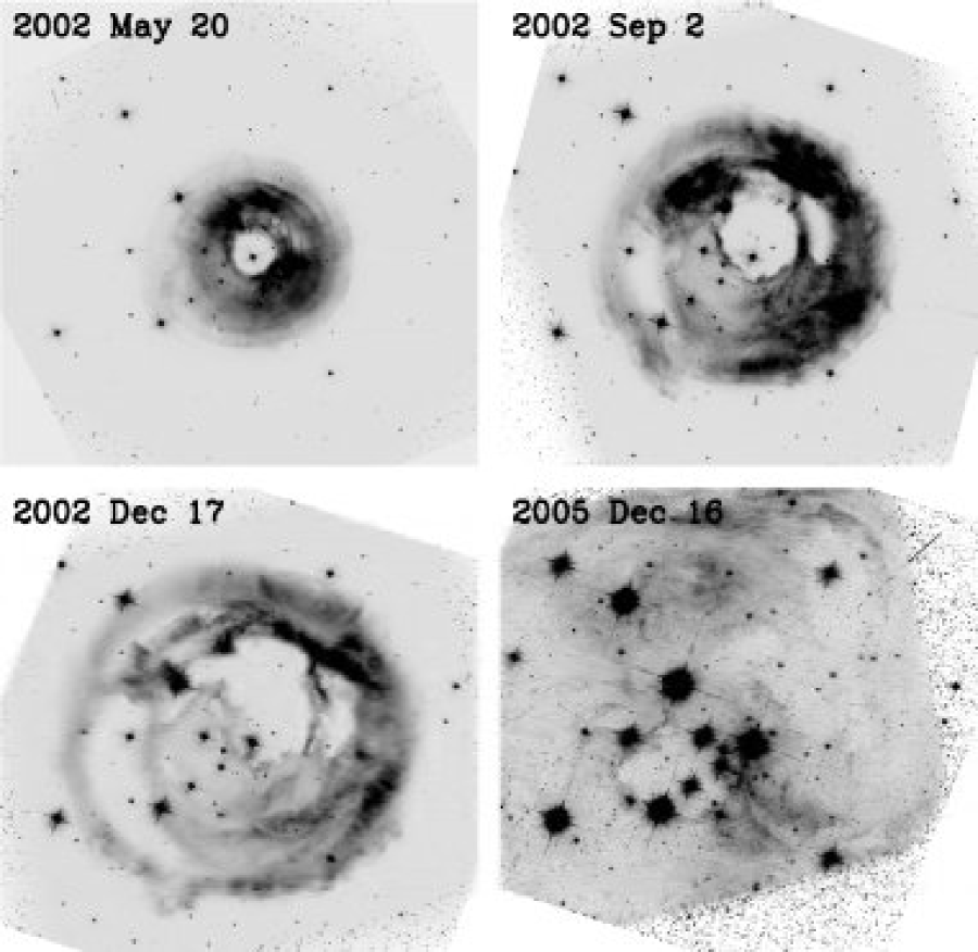
Figure 1: Total-intensity (i.e., Stokes $I$) HST ACS images of the V838 Mon light echo in the $V$ (F606W) filter for each of the four epochs of polarimetric data. The images have been rotated to place north up and east on the left, and each frame is $97^{\prime\prime}$ wide. Polarimetric observations were obtained on 2002 May 20, September 2, and December 17, and on 2005 December 16, as labelled in the figure. The image stretch is linear, and the fading of the light echo has been compensated by scaling the image intensities. V838 Mon itself is located near the center of the cavity in the 2002 May 20 image.

In Fig. 1 we show pictorial representations of the total-intensity (i.e., Stokes $I$) images of V838 Mon at the four epochs of $V$-band HST polarimetric imaging. The sequence of three images from 2002 shows the rapid apparent increase in size of the echo from May through December, and by 2005 the echo was larger than the FOV of the ACS polarimetry mode. For the 2002 images we placed V838 Mon at the center of the FOV. In 2005, however, since we anticipated that the diameter of the light-echo polarization ring would be larger than the size of the FOV, we placed the star near a corner of the FOV.

In Fig. 2 we use image brightness to represent the linear-polarization degree, $p$. Here we see that the complex structures seen in the intensity images of Fig. 1 give way to a smooth, azimuthally symmetric morphology, just as expected from a straightforward scattering configuration. The 2002 May image shows that the linear polarization increases inward toward the star, but does not reach a maximum before encountering the prominent cavity surrounding the star. Hence this image can be used only to derive an upper limit to the radius of the polarization ring, and thus only a lower limit to the distance to the star. By 2002 September, it appears that the peak of the polarization ring has been reached only on the south side of the star, but not elsewhere, where the cavity radius measured from the central star is larger. By 2002 December, and also in 2005, there is dust present at many azimuths that contain the maximum of the polarization ring. In the latter two images, the percent polarization at the ring location is extremely high, approximately 50%, as expected for light scattered at $90^{\circ}$ off small particles (e.g., White 1979).

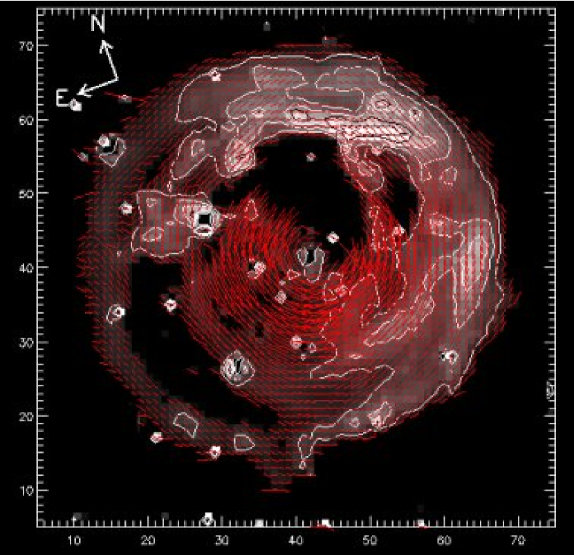
Figure 3: The echo image of 2002 December 17 (contours and greyscale image) with polarization electric vectors superimposed. The directions of the electric vectors are indicated by the red lines, whose lengths are proportional to the degree of polarization. The largest values are about 50%. Vectors are shown every 30 pixels, and the polarization and position angles are the means and medians, respectively, averaged over $30\times 30$-pixel boxes. This image has not been rotated to place north at the top, but instead remains in detector coordinates. Small tickmarks on the axes are separated by $1\farcs 5$. Note that the electric vectors are generally perpendicular to the direction to the central star, as expected for light scattered off dust particles.

In Fig. 3 we represent the linear polarization in the image of 2002 December 17, using red line segments, which are oriented to show the direction of the electric vectors, and whose lengths are proportional to the degree of polarization. Here we have left the image in detector coordinates and orientation, rather than rotating it to place north at the top as in Figs. 1 and 2. The electric vectors are seen generally to be oriented perpendicular to the direction to the central star. Again, this behavior is just as expected for dust scattering, and it strongly confirms both the dust-scattering nature of the light echo and our data-reduction procedures.

3.5 Cleaning the Polarimetric Images

For comparison to dust-scattering models of the light echo, and before using the polarimetry to determine the distance to the star, it was necessary to carry out two steps of cleaning the basic polarization images presented above. First, we wished to accept only data of good signal-to-noise (S/N) ratio level. The polarization uncertainties are provided by our noise model as described above, and we chose to reject regions of the polarization-degree images having a 1$\sigma$ uncertainty in $p$ greater than 10% of the value of $p$. In order to retain an acceptable fraction of useful data, we first box-car smoothed the 2002 data using a $7\times 7$-pixel box before the S/N-rejection process. In 2005 December the echo was much fainter, and we used $11\times 11$-pixel smoothing.

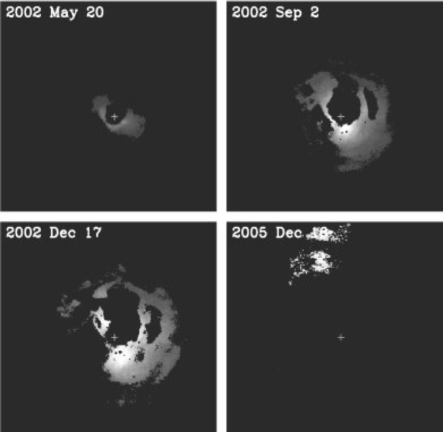
Figure 4: The images illustrating polarization degree shown in Fig. 2 are here masked to retain only regions free of stars and with linear polarization degree detected with $\rm S/N>10$, as described in the text. Image scale, orientation, and stretch are the same as in Fig. 2. The location of V838 Mon in each masked image is marked with a white cross.

Second, the presence of a substantial number of stars in the FOV complicates the analysis. For each epoch, we generated a catalog of the field stars, measured their fluxes, and generated an artificial star-field image from the catalog using an empirical PSF derived from stars clear of the echo. Many of the stars are significantly saturated, so our photometric procedure used a correction for saturation based on the ratio of flux in an unsaturated annulus to the total flux. For the same reason, a composite empirical PSF was used that combined the broad halo of a saturated star with the core region of a different star with much reduced saturation. Then, following the same principles as in the previous paragraph, we eliminated regions of the data where the stellar halos exceeded 10% of the total Stokes $I$ intensity (which would introduce a 10% error in $p$). Beyond the stellar image cores, in the region where the halo has less than a 10% influence on polarization, we subtracted the estimated stellar halo from the Stokes $I$ image and corrected the polarization-degree image accordingly for this small effect. Fig. 4 shows the result of masking out regions with $\rm S/N<10$ and regions near bright stars, as described above, for each of the four epochs.

4 Modeling the Light Echo

4.1 Outburst Light Curve

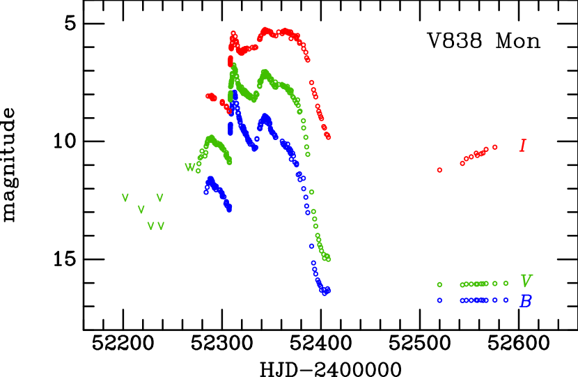
Figure 5: Outburst light curves adopted for V838 Mon in the ground-based Johnson-Kron-Cousins $B$, $V$, and $I$ bandpasses, colored blue, green, and red respectively. “V” signs mark upper limits before the onset of the outburst. The data are the same as used by Bond et al. (2003), but are plotted here as stellar magnitudes rather than on a linear flux scale.

We next need to know the time behavior of the echo illumination due to the outburst of V838 Mon. Fig. 5 shows the light curves that we adopted. These are ground-based Johnson-Kron-Cousins $B$, $V$, and $I$ magnitudes, which are presented as a function of time. They are taken from a variety of ground-based sources, and are the same data used in Bond et al. (2003), which can be consulted for the original references.

We then estimated the equivalent ACS count rates in the F435W, F606W, and F814W filters, using the equations in Sirianni et al. (2005). These are the total count rates from the star in electrons s^-1 that ACS would have detected throughout the eruption.

To characterize the light curve and outburst, we derived several fiducial characteristic quantities, as follows. For modeling purposes, we used only the portion of the light curve between $(\rm HJD-2400000)=52307$ and 52404, that is, the 97-day interval from 2002 February 2 to May 10. This interval excludes the initial precursor rise prior to the sudden peak in early February; however all of the flux emitted in the 32 days before February 2 constitutes only about 3.9% of the total emitted flux, and its omission significantly reduces the complexity of our analysis. Over the 97 outburst days, the derived average count rate in the F606W plus POLV filter was $1.14\times 10^{7}$ counts s^-1, and the total counts emitted over the 97 days was $9.55\times 10^{13}$. The flux-averaged mean Johnson $V$ magnitude is $\langle V\rangle=7.95$. The peak-brightness Johnson $V$ magnitude is $V_{\rm max}=6.77$, with a peak ACS F606W count rate of $2.89\times 10^{7}$ counts s^-1. Thus the total emitted flux is equivalent to the $V_{\rm max}$ brightness shining for 38 days. The intensity-weighted mean date of the outburst is HJD 2,452,343, or 2002 March 9. Hence, the four epochs of our F606W polarimetric imaging correspond to times after the outburst mean of about 72, 177, 282 and 1377 days. Note that, for the first epoch, the outburst had ended, with the above conventions, only 9 days earlier.

4.2 Three-Dimensional Geometry and Appearance of the Light Echo

As a prelude to the polarization analysis, it is useful to visualize the geometry of the light echo at each of the epochs of observation. Figure 6 shows the geometric configuration at the four epochs. Anticipating the results below, we show the locations of the light-echo paraboloids for an assumed distance of 6.1 kpc. The observer lies in the direction of the $+z$ axis. The linear distances on the $x$ axis have been converted to WFC pixels, whose $0\farcs 05$ pixel scale corresponds to 0.0015 pc at the adopted distance. The $z$ distances are shown in the same units.

Due to the protracted duration of the outburst, the dust illuminated at a given epoch spans a significant depth in the LOS, especially at the earlier epochs. For each of the four epochs, Figure 6 shows light from the beginning of the outburst as dashed lines, and light from the end (97 days later) as solid lines. Along each LOS, the scattering material is illuminated by a replica of the complete light curve, which is somewhat distorted because of the non-linear mapping of $t$ to $z$.

Figure 6 shows that, for almost any assumed distribution of clumpy dust, the LOS at a larger projected separation $x$ from the star corresponds to light emitted earlier in the outburst. Thus, since the earliest light was much bluer than light emitted toward the end of the outburst (see Figure 5), we generally expect to see outer blue rims in the light echo.

Figure 7 shows a color rendition of the 2002 December 17 observations prepared by one of us (Z. L.) by combining the images in $B$ (F435W), $V$ (F606W), and $I$ (F814W). This representation bears out beautifully the expectation described above, since it shows numerous outer blue rims throughout the light echo. This color information will allow us to determine three-dimensional depths for the dust clouds, which will be done in a separate paper.

4.3 Quantitative Source Functions for the Echo

In order to model the polarization distribution of the echo, we began by combining the light-curve data given in §4.1 and plotted in Fig. 5 with the three-dimensional geometry described in §4.2 and illustrated in Fig. 6, to produce a set of source functions. These are two-dimensional functions (projected distance from the star and line-of-sight distance), with rotational symmetry assumed for the third dimension. The source functions were then integrated along the LOS to produce simulated polarization and intensity curves for comparison with the actual data.

For each LOS at each radius at each of the four epochs, we first established the range of $z$ distances that corresponded to the beginning and end of the outburst, as shown in Fig. 6. This $z$ range was then divided into equally spaced sampling points, each of which corresponds to a particular time during the outburst. Next we interpolated in the light curve to determine the flux illuminating each of these $z$ volume elements (“voxels”). The illuminating flux is given by $L(t)/4\pi d^{2}$, where $L(t)$ is the luminosity of the star at time $t$ and $d$ is the distance of the voxel from the star.

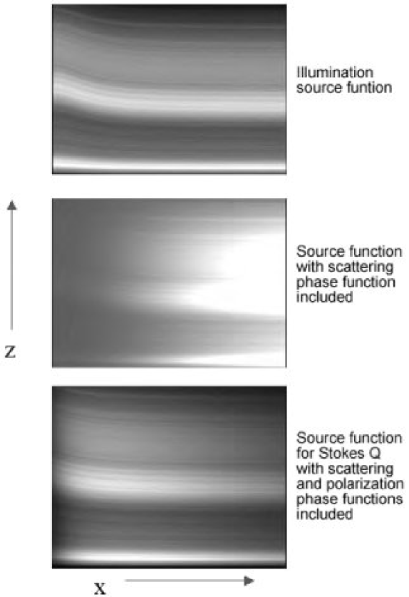
Figure 8: Source functions for the V838 Mon light echo, illustrated for a particular stellar distance (6.1 kpc) and epoch (2002 December 17). In each panel the source functions are represented by brightness as functions of projected $x$ distance from the star, and $z$ depth in the line of sight on a linear distance scale from the largest time lag (bottom of each panel) to the smallest lag (top of each panel). The top panel shows the illumination function from the outburst light curve; the middle panel also includes the dust scattering function; and the bottom panel adds the polarization function. See text for details. Such source functions were constructed for all four epochs and for a large range of plausible stellar distances.

Figure 8 gives an illustration of the steps in the calculation of the source functions. The top panel shows a representation of the illumination function for the 2002 December 17 epoch. The horizontal axis is projected distance from the star, and the vertical axis corresponds to distance along the $z$ axis toward the observer, plotted on a linear distance scale from the largest time lag at the bottom to the smallest lag at the top. As illustrated in Fig. 6, the physical length along the $z$ axis increases from left to right. The thin, nearly horizontal stripe at the bottom of the illumination function corresponds to the initial sharp spike in the light curve, and then moving up we see the subsequent dip in brightness, followed by a second brightening and then the final fading. The distortion of the light curve, especially noticeable at small projected $x$ distances, is due to the parabolic geometry of the echo.

Next we included the angular dependence of the efficiency of light scattering off small particles. We adopted the usual Henyey-Greenstein (1941) phase function

$$\Phi(\theta)=(1-g^{2})/[4\pi(1+g^{2}-2g\cos\theta)^{3/2}]\,,$$

where $\theta$ is the scattering angle, with $\theta=0^{\circ}$ corresponding to forward scattering. This function contains a parameter $g$, for which we adopt the empirical value of $g=0.6$ (e.g., White 1979; Draine 2003). The second panel in Figure 8 shows the effect of including the scattering phase function. Here we see the enhancement of the source function at larger values of $x$, where, because of the parabolic geometry, we are closer to the highly efficient forward-scattering regime.

Finally, we included the dependence of degree of linear polarization on scattering angle. We chose the classical polarization function for Rayleigh scattering,

$$p=p_{\rm max}\,(1-\cos^{2}\theta)/(1+\cos^{2}\theta)$$

(e.g., Born & Wolf 1980, section 13.5.2), which has its maximum value of $p_{\rm max}$ at $\theta=90^{\circ}$. In the calculations below, we take $p_{\rm max}$ to be a free parameter. For pure Rayleigh scattering, $p_{\rm max}=1$, but in typical astronomical situations it is smaller. The bottom panel in Figure 8 shows the final source function with this factor included. We now see all of the contributors along the LOS to the value of the Stokes $Q$ parameter. The axial symmetry of the echo geometry means there is no loss of generality from computing only one of the two linear-polarization parameters, $Q$ and $U$.

We can now integrate along the $z$ axis of each LOS, with the contributors to the surface brightness in Stokes $I$ given by

$$dI(z)=n_{H}(z)\,\omega\sigma\{L(t)\Phi(z)/(4\pi d^{2}D^{2})\}dz\,,$$

and those to Stokes $Q$ by

$$dQ(z)=n_{H}(z)\,\omega\sigma p_{\rm max}\{L(t)\Phi(z)/(4\pi d^{2}D^{2})\}\{(1-\cos^{2}\theta)/(1+\cos^{2}\theta)\}dz\,,$$

where $n_{H}(z)$ is the volume density of hydrogen atoms, $\omega$ is the dust albedo, and $\sigma$ is the scattering cross-section per atom. We take $\omega=0.6$ (Mathis, Rumpl, & Nordsieck 1977) and $\sigma=4.4\times 10^{-22}\,\rm cm^{2}$ at 6000 Å (Savage & Mathis 1979). $L(t)$ is the time-dependent luminosity of the star, and $\Phi(z)$ is the phase function for the scattering angle $\theta$ corresponding to depth $z$. The terms in curly braces may be recognized as the intensity, scattering, and polarization source functions, with additional normalization for the distance $D$ of V838 Mon.

Quantitatively, we used units of ACS count rate for the term $L(t)/(4\pi D^{2})$, which is the flux that V838 Mon itself would have had, if it had been observed throughout its outburst by the ACS. (This is the light curve computed in §4.1.) With this definition, summation of the voxels along each LOS yielded an ACS count rate for each spatial pixel for an assumed constant density of $n_{H}=1\,\rm cm^{-3}$. Note that comparison of the integrated intensity with the observed count rate yields an average density at each position, which will be the subject of a separate paper.

To generate a polarization model for comparison with the data, we calculated the contribution to Stokes $Q$ for each voxel in a similar fashion, and also summed these along the LOS, assuming constant density. Division of the integrated Stokes $Q$ function by the integrated intensity $I$ yielded a model polarization degree, which was used for comparison with the data. Strictly speaking, the polarization will depend on the density distribution, as this influences the average intensity-weighted scattering angle along the LOS. However, these integrations are only along a relatively narrow range in $z$, as shown in Fig. 6. The total range of scattering angle along any given LOS for the 2002 December echo geometry is less than $20^{\circ}$, and is typically in the range 10–20^∘. Further, given a random distribution of dust clouds, we expect the azimuthal averaging process to bring the actual average scattering angle for a particular radius close to the idealized mean value of the models. A grid of models was computed in this way for each epoch and for a range of distances from 4 to 12 kpc.

5 Geometric Distance

5.1 Polarization Profiles

Figure 9 shows plots of the azimuthally averaged degree of polarization vs. radius for the F606W polarimetric observations obtained in 2002 September and December. These curves were calculated from the fully cleaned $7\times 7$-binned polarization images, derived as described in §§3.3-3.5, and illustrated in Figure 4. The azimuthal averages were calculated for annuli centered on V838 Mon.

The 2002 September data show a polarization maximum fairly close to the outer edge of the central cavity around the star (see Fig. 1, upper-right panel). By the time of the 2002 December observation, this maximum had moved to a larger radius and had become well defined. The overall appearance of both the polarization maps in Figure 4 and the azimuthally averaged polarization profiles in Figure 9 is encouragingly smooth. This appearance is quite similar to expectation (e.g., Sparks 1994, 2005), with a central dark hole, a smooth and fairly wide maximum, and a shallow outer decline in polarization. The light echo is about 50% linearly polarized at the location of the maximum.

To derive a geometric distance, we begin with simple approximations and work through to a detailed numerical analysis which takes into account the extended duration of the outburst and the dust scattering and polarization properties.

5.2 Approximate Estimates

First, to obtain a sense of the approximate distance implied by these data, we located the peaks of the polarization rings for 2002 September and December. This was done by fitting parabolas to the peaks depicted in Figure 9, using only polarization values greater than 0.4. The distance then follows by equating the angular radius of the peak location to a linear radius of $ct$. We find the respective peaks to lie at radii 99 and 167 pixels, corresponding to angular radii of $4\farcs 95$ and $8\farcs 35$. Adopting an instantaneous approximation to the outburst light curve, and delay times of $t=177$ and 282 days (cf. §4.1), these radii imply distances of $6.19\pm 0.29$ and $5.85\pm 0.13$ kpc, where the uncertainties are the formal fitting errors and do not include systematic uncertainties. The peak degrees of polarization are 48.5% and 48.8%, respectively.

The apparent outward motion of the polarization peak can also be used to obtain a distance, without knowing the outburst date, by setting the angular motion to a linear motion at the speed of light (e.g., Sparks 1997). The measured motion of $3\farcs 40$ in 105 days implies a distance of $5.36\pm 0.47$ kpc. The uncertainty is higher here since the errors on both individual measurements combine quadratically.

5.3 Detailed Modeling of the 2002 September and December Data

Our detailed modeling concentrated initially on the observations of 2002 December. We compared the full azimuthally averaged polarimetric data to model polarization curves determined numerically as described in §4, for a range of assumed distances $D$ and fitting $p_{\rm max}$ as a free parameter. Fig. 10 shows three examples of such fits to the 2002 December data. For each distance we computed the rms residuals of the model fit to the polarization data, and found a well-defined minimum corresponding to a distance $D=5.69$ kpc. The best-fit value of $p_{\rm max}$ at this distance is 53.7%. This best model polarization curve is the middle one plotted in Fig. 10, which also illustrates the rapid degradation of fit quality away from the best-fit distance.

Applying the same procedure to the 2002 September data, we found a very similar best-fitting distance of 5.59 kpc, with $p_{\rm max}=51.7\%$. The best fits to the 2002 September and December data are shown together in Figure 11.

To test the robustness of this approach, and reduce sensitivity to the shape of the broad, low-polarization wings, we also derived rms residuals restricting the models and data just to regions where the polarization degree was greater than 0.4, i.e., fitting the models just to the peak of the curve. For the 2002 December data, the best-fit distance increased slightly to 5.79 kpc from the 5.69 kpc of the fit to the whole curve, and for 2002 September it increased from 5.59 to 5.84 kpc. The peak polarizations are 51.3% and 50.5%, respectively.

One reason that the derived distance depends on the $p$ cutoff value is that, as Fig. 11 shows, the observed polarization curves depart somewhat from the Rayleigh-type model curves: the models have sharper and higher peaks, and they decline more rapidly with radius than the actual data. Hence we turn to a different way of looking at the data, which is to adopt a distance and then derive the polarization degree as a function of scattering angle which is implied by the data. In other words, we derive the empirical polarization phase function that would be implied at each assumed distance. This approach makes use of the fact that the assumed distance defines the relationship between angular radius and scattering angle. Such phase curves have the advantage that we expect them to be quite symmetric, unlike the significantly asymmetric spatial polarization curves, given the exactly symmetric Rayleigh phase function $p/p_{\rm max}=(1-\cos^{2}\theta)/(1+\cos^{2}\theta)$. A second advantage is that we are now making a simpler and more direct comparison with a basic physical property of the dust.

For each numerical model, at each assumed distance, we calculated the intensity-weighted mean scattering angle as a function of radius, taking into account the geometry, light curve, and scattering functions described above. We then plotted the observed degree of polarization against this mean scattering angle. Fig. 12 shows examples of empirical scattering curves derived for assumed distances of 4, 6, and 8 kpc from the 2002 December data. It is apparent from Fig. 12 that the effect of assumed distance on the polarization scattering function is indeed to move the location of the peak. For reference we also show the Rayleigh phase function as a smooth curve in Fig. 12.

We fitted parabolas to the peaks of the phase functions, using only polarization values $p>0.3$, in order to derive the locations of the peaks as a function of assumed distance. The results are shown in Fig. 13, which again shows that the derived distance decreases with increasing $\theta_{\rm max}$. To estimate the distance geometrically, we return to the basic assumption that polarization maximizes at a scattering angle of $90^{\circ}$. The 2002 December curve (solid line in Fig. 13) intersects $90^{\circ}$ for a distance of 6.07 kpc. The 2002 September data (dashed line) give a nearly identical distance of 6.12 kpc. We may ask how robust is our assumption that the polarization maximum occurs at $90^{\circ}$. Laboratory measurements of a variety of mineral dust particles typically give polarization maxima in the range $90^{\circ}$–$100^{\circ}$ (Dumont 1973; Muñoz, Volten, & Hovenier 2002), while cometary dust is found empirically to have a maximum polarization of about 30% at about $90^{\circ}$ (Moreno, Muñoz, & Molina 2002 and references therein). Theoretically, White (1979) used Mie theory to calculate the scattering properties of the Mathis et al. (1977) grain distribution. His analysis yields $\theta_{\rm max}$ values between $88^{\circ}$ and $95^{\circ}$ at wavelengths of 6000–6500 Å. On this basis we adopt $\theta_{\rm max}=90^{\circ}\pm 5^{\circ}$ as a reasonable estimate of the angle of maximum polarization and its systematic uncertainty.

In the case of an instantaneous outburst, it can be shown that the actual distance is given exactly by $D=D_{90}(1+\cos\theta_{\rm max})/\sin\theta_{\rm max}$, where $\theta_{\rm max}$ is the actual scattering angle for maximum polarization and $D_{90}$ is the distance derived assuming $\theta_{\rm max}=90^{\circ}$. We overlay this function in Figure 13 for $D_{90}=6.1$ kpc, where it may be seen that this analytical expression is very close to the numerical model. In the neighborhood of $\theta_{\rm max}=90^{\circ}$, the derived distance decreases by 1.7% for each one-degree increase in $\theta_{\rm max}$.

Thus, if the peak polarization were to occur $5^{\circ}$ on either side of $90^{\circ}$, the derived distance would change by about 9%, corresponding to a distance range of 5.5 to 6.7 kpc. This conclusion is robust to the cut-off polarization degree assumed, as might be expected from the smooth and roughly parabolic nature of the phase curves, as shown in Fig. 12.

Next we tried the experiment of adopting the polarization phase function implied by the 2002 September observations, and then using it to predict the spatial distribution of polarization for the scattering-angle distribution at the time of the 2002 December observation. The results are nearly independent of distance and are shown in Fig. 14, which tests how consistent the polarization profiles derived at the two epochs are. In fact, the consistency between the predicted and observed curves is remarkably good.

In Fig. 15 we show the polarization phase curves derived from the 2002 September and December data for an adopted distance of 6.1 kpc, corresponding to $\theta_{\rm max}=90^{\circ}$. The two phase curves are nearly identical, which lends considerable confidence to our analysis methods.

As shown in Fig. 15, we fitted parabolas to the two phase functions, using only the portions with $p>0.3$. We then used the parabolic phase functions to predict the spatial polarization profiles at the 2002 September and December epochs. Fig. 16 compares these predictions with the actual data. The fit to the observed peaks is excellent.

5.4 The First and Fourth Epochs

Polarization observations in the F606W filter were also obtained in 2002 May and 2005 December, as described in §2 and summarized in Table 1. The 2002 May data are unsuitable for distance measurement because the location of polarization maximum was well within a cavity in the light echo at that epoch.

The data from 2005 December were also processed as described above. At that late epoch, the echo was of much lower surface brightness than in 2002, and relatively little of the image has polarization degree measured at high S/N, as illustrated in Figs. 2 and 4. Hence a distance derived from such data would be liable to significant uncertainties. Instead, we content ourselves with a comparison of the observed polarization to what is expected based on the results of the late-2002 analysis. Fig. 17 shows the predicted polarization degree as a function of projected radius. The predictions are based on the same line-of-sight integrations described above, the Rayleigh formula for the polarization phase function, and an assumed distance of 6.1 kpc. We found that a slightly higher maximum polarization degree of 0.55 instead of 0.5 appeared to provide a better description of the data, but otherwise Fig. 17 shows that the 2005 data are reasonably consistent with the results obtained from the 2002 data.

6 The Distance and Nature of V838 Mon

The uncertainty in our final distance estimate is dominated by systematic errors, with the primarily source being the uncertainty in the scattering angle that produces maximum linear polarization. As discussed in §5.3, we adopted $\theta_{\rm max}=90^{\circ}\pm 5^{\circ}$. This leads to our final best estimate of $D=6.1\pm 0.6$ kpc.

Initial estimates of the distance to V838 Mon ranged over more than an order of magnitude. Shortly after the appearance of the light echo, a very short distance ($\sim$0.7 kpc) was derived under the assumption that the outer edge of the echo lies at a projected radius of $ct$ (e.g., Munari et al. 2002; Kimeswenger et al. 2002). As explained by Munari et al. (2005), the implicit assumption had been made that the dust formed a face-on disk around the star, but we now know that this is not the case. In fact, the apparent expansion rate of a light echo is almost always superluminal. Using the proper paraboloidal geometry, Bond et al. (2003) showed, from the apparent expansion rates of the echo, that the distance must be substantially larger than 2 kpc.

As V838 Mon declined in visual light in late 2002, spectroscopic observations revealed an unresolved B3 V companion star (Munari & Desidera 2002; Wagner & Starrfield 2002). Giving high weight to a spectroscopic parallax of the B3 companion, Munari et al. (2005) favored a much larger distance of $\sim$10 kpc. However, Afşar & Bond (2007) have argued that this is an overestimate because the B star suffers extinction over and above that due to the foreground interstellar medium; this extra extinction would be due to the B star lying within (or behind) dust ejected from V838 Mon during the 2002 outburst. This argument appears to have been confirmed by recent dramatic episodes of fading of light from the B3 star (Goranskij 2006; Bond 2006; Munari et al. 2007), attributed to dust from V838 Mon engulfing or passing in front of it.

A more reliable distance comes from the discovery by Afşar & Bond (2007) that V838 Mon belongs to a sparse young cluster, containing three B-type stars in addition to the unresolved B3 companion. By photometric main-sequence fitting of the three B stars, Afşar & Bond find a reddening of $E(B-V)=0.85$ and a distance of $6.2\pm 1.2$ kpc. The agreement with the polarimetric distance of $6.1\pm 0.6$ kpc is excellent. We are attempting to identify more members of the cluster in order to refine the distance estimate, which would provide additional support for our assumption of $\theta_{\rm max}=90^{\circ}$ in the polarization analysis.

The apparent magnitude of V838 Mon at its maximum in early 2002 February was $V=6.77$ (see Fig. 5). At a distance of 6.1 kpc, and for the reddening given above, the absolute magnitude at maximum was an extraordinary $M_{V}=-9.8$, making V838 Mon temporarily one of the visually brightest stars in the entire Local Group (e.g., Humphreys 1983, Table 3). V838 Mon was brighter at maximum than all but the very fastest of classical novae (e.g., Downes & Duerbeck 2000, their Fig. 17).

In 1988, a luminous cool object appeared in the nuclear bulge of M31. This object, called the “M31 red variable” or “M31 RV,” is widely considered to be an analog of V838 Mon (e.g., Bond & Siegel 2006 and references therein). Photometric coverage of its outburst, collected by Boschi & Munari (2004, their Table 5), was unfortunately fairly sparse, especially in the $V$ band. However, by combining the brightest observed $B$ magnitude, $B=17.3$, with a color index of $B-V=1.89$ observed later in the outburst, we can estimate $V_{\rm max}\simeq 15.4$. Adopting $E(B-V)=0.12$ and $(m-M)_{0}=24.48$ for M31 RV from Boschi & Munari, we find $M_{V\rm,max}\simeq-9.4$, similar to the maximum brightness of V838 Mon.

The Galactic star V4332 Sgr is a third object that was also a red supergiant throughout its outburst (Martini et al. 1999; Tylenda et al. 2005 and references therein). Its distance is, however, poorly constrained.

The outburst mechanism for this new class of objects remains uncertain. Their outburst behavior, featuring a rapid expansion to a very cool, luminous supergiant, is unlike that of any previously known type of variable star. A thermonuclear runaway on a white dwarf in a nova-like system is probably ruled out by the very young age of the cluster surrounding V838 Mon, $<$25 Myr (Afşar & Bond 2007), which appears to be too short to allow formation of a close binary containing a white dwarf. An explosive event in a massive star seems to be excluded by the fact that the population surrounding M31 RV contains only old red giants (Bond & Siegel 2006). The high luminosities and rapid expansion timescales appear to disallow a “born-again” event in a low-mass pre-white dwarf.

Thus recent discussions of these objects have concentrated on stellar-merger scenarios (e.g., Tylenda & Soker 2006 and references therein) and even planet-star mergers (e.g., Retter et al. 2006). Mergers have the advantage of possibly occurring in both young and old populations. Moreover, they lead to an expectation of a wide range of outburst luminosities, determined by the potentially wide range of parameters of the merging objects. This expectation appears to be borne out by the recent discovery of an apparently V838 Mon-like event in the Virgo galaxy M85 (Rau et al. 2007; Kulkarni et al. 2007), which, at a peak absolute magnitude of $M_{V}\simeq-13$, was at least $\sim$20 times more luminous than V838 Mon and M31 RV at maximum.

A related issue, which also bears on outburst mechanisms for V838 Mon, is the origin of the dust being illuminated in the light echo. Different authors have argued that the dust was ejected from V838 Mon in a previous outburst, or that it is ambient interstellar dust whose origin is unrelated to V838 Mon itself. If the dust did come from a previous outburst, it would cast doubt on the stellar-merger scenarios, which presumably would be one-time events. These issues do not affect our distance determination, and are thus beyond the scope of the present paper; see the recent conference proceedings for discussions of the origin of the dust (Corradi & Munari, eds., 2007).

7 The Utility of Light Echoes for Geometric Distance Measurement

The use of light-echo polarimetry to obtain geometric distances of supernovae (SNe) was proposed by Sparks (1994). The method has now found its application to the distance to an extraordinary outburst event within the Milky Way. The result agrees extremely well with the distance obtained from a completely independent, classical method of cluster main-sequence fitting, thus providing strong support for the validity of the polarimetric technique.

SN light echoes offer the prospect of geometric distance measurements on an extragalactic scale. In fact, SNe form a more favorable class of object than V838 Mon, because of the short outburst timescale, and because SNe are intrinsically extremely bright and can potentially illuminate bright, long-duration light echoes. However, there must be interstellar dust distributed sufficiently in the vicinity of the SN to produce both a light echo and a clear maximum of linear polarization, corresponding to the dust lying in the plane of the sky.

The angular diameter of the linear-polarization ring in a SN light echo (corresponding to a linear diameter of $2ct$) is given by $\theta=0\farcs 126\,(t/{\rm 1\,yr})\,({\rm 1\,Mpc}/D)$. Such sizes make the polarimetric method feasible with ground-based techniques within and perhaps slightly outside the Local Group. At HST resolution, geometric distance measurements to galaxies within several Mpc should be feasible. In fact, linear polarization was detected in HST polarimetry of a light echo around SN 1991T in the Virgo galaxy NGC 4527; modeling of the polarization (Sparks et al. 1999) showed consistency with a distance of $\sim$15 Mpc, but these images, taken at $t\simeq 6$–8 yr after the outburst, only marginally resolved the echo.

8 Conclusions

We have applied the method of light-echo polarimetric imaging described by Sparks (1994) to the derivation of a geometric distance to V838 Mon. Following a careful reduction of polarimetric images of the light echo, obtained with the Advanced Camera for Surveys onboard the Hubble Space Telescope, we confirmed the presence of an apparently expanding ring of highly polarized light surrounding V838 Mon. Setting the radius of this ring to a linear size of $ct$ yielded initial distance estimates of 5.4–6.2 kpc. We then developed modeling and fitting procedures of increasing complexity, which yielded consistent results.

Our final best value for the distance is $6.1\pm 0.6$ kpc, where the error is dominated by the systematic uncertainty in the scattering angle of maximum linear polarization. This distance agrees extremely well with a value of $6.2\pm 1.2$ kpc, obtained by an entirely independent method of main-sequence fitting, applied to a sparse stellar cluster to which V838 Mon belongs.

At this distance, the outburst of V838 Mon in early 2002 is shown to have been extremely luminous—it was brighter than all but the most luminous classical novae, and temporarily one of the brightest stars in the entire Local Group. The mechanism that produced such an outburst remains uncertain, but scenarios involving stellar mergers may be the most plausible.

Our results strongly verify the polarimetric method for determining geometric distances. The technique shows great promise for application to distance determinations for extragalactic supernovae.

Figure 2: Images representing the degree of linear polarization, $p$, for each of the four epochs of data shown in Fig. 1. Image scales and orientations are the same as in Fig. 1. The image stretch is linear, ranging from black representing zero linear polarization to full white representing $\sim$50% linear polarization. These images illustrate the apparent outward motion of a ring of highly polarized light in the light echo.

Figure 6: Spatial locations of the light-echo paraboloids for our four epochs of F606W polarimetric imaging. The observer is located on the $+z$ axis, V838 Mon lies at the (0,0) origin, and the $x$ and $z$ distances from the star are in units of ACS pixels ($0\farcs 05$) for an adopted distance of 6.1 kpc. The 850-pixel width of the diagram corresponds to a linear width of 1.26 pc. At each epoch, the solid line marks light from the end of the outburst (shortest time delay), and the dashed line marks the beginning of the outburst (longest time delay). Blue represents the paraboloids for 2002 May, green for 2002 September, red for 2002 December, and cyan for 2005 December.

Figure 7: Color rendition of the V838 Mon light echo on 2002 December 17, prepared from the HST $B$, $V$, and $I$ images listed in Tables 1 and 2. Note the prevalence of blue outer edges and red inner ones, which arise as a consequence of the echo geometry and the time behavior of the outburst light, as described in the text. The image is $90^{\prime\prime}$ high and has north at the top and east on the left.

Figure 9: Azimuthally averaged polarization profiles for 2002 September and December, including only data for the regions illustrated in Fig. 4.

Figure 10: Azimuthally averaged polarization data for 2002 December (noisy line) compared with numerical model Rayleigh-type polarization scattering functions for distances of 8, 5.7, and 4 kpc (smooth curves). The best fit is for 5.7 kpc.

Figure 11: Azimuthally averaged polarization data for 2002 December (right-hand noisy line) with best-fit Rayleigh-type polarization scattering function for a distance of 5.7 kpc (right-hand smooth curve), both repeated from Fig. 10. Also shown are the data (left-hand noisy line) and a similar fit (left-hand smooth curve) for the 2002 September polarimetric data, which yield a best-fit distance of 5.6 kpc.

Figure 12: Linear polarization degree plotted as a function of scattering angle, as derived for the 2002 December data and assumed distances of 8 kpc (inner curve), 6 kpc (middle noisy curve), and 4 kpc (outer curve). If V838 Mon lies at a distance of 4 kpc, peak linear polarization occurs at a scattering angle of $\sim$$110^{\circ}$. If it is at a distance of 8 kpc, the peak is at an angle of $\sim$$75^{\circ}$. For reference the smooth curve shows a standard Rayleigh polarization curve given by $p/p_{\rm max}=(1-\cos^{2}\theta)/(1+\cos^{2}\theta)$, with $p_{\rm max}=0.5$, which peaks at a scattering angle of $90^{\circ}$.

Figure 13: Derived scattering angle for peak polarization as a function of distance. The solid line shows the result for the 2002 December data, and the dashed line for the 2002 September data. The dotted curve is the analytic solution for an instantaneous outburst with $D_{90}=6.1$ kpc. The horizontal dotted line shows a $90^{\circ}$ scattering angle, which intersects both observed curves at a distance of 6.1 kpc.

Figure 14: Result of mapping the 2002 September polarization profile forward to its equivalent in 2002 December, using the phase function (i.e., the relationship between polarization and scattering angle) implied by the September data. The left-hand curve is the observed polarization profile in 2002 September. The right-hand curve is the profile predicted for 2002 December using the September phase function. The dashed line on the right is the actual December data.

Figure 15: Polarization as a function of scattering angle (“polarization phase curves”) derived from the 2002 September and December data (dotted and dashed lines, respectively). The adopted distance is 6.1 kpc, which yields a peak polarization at a scattering angle of $90^{\circ}$. The solid curves show parabolic least-squares fits to the two data sets for values of $p>0.3$ only.

Figure 16: Polarization as a function of radius for the 2002 September and December epochs, calculated for the phase functions represented by the parabolic fits shown in Fig. 15 (smooth curves). The actual data are shown as noisy curves.

Figure 17: The crosses show the azimuthally averaged polarization profile for 2005 December 16, based on the masked data shown in Fig. 4. The smooth curve is the predicted profile, calculated using the polarization phase function of 2002 December 17 and an assumed distance of 6.1 kpc. Here $p_{\rm max}$ was set to 0.55 rather than 0.5, but otherwise the observations are reasonably consistent with expectation.

Table 1: Log of HST ACS WFC Polarimetric Observations of V838 Mon

Dataset	UT Date	Exposure (s)	Filters	Proposal ID & PI
J8GG01011	2002 Apr 30	506	F435W;POL0UV	9587 Starrfield
J8GG01021	2002 Apr 30	506	F435W;POL60UV	9587 Starrfield
J8GG01031	2002 Apr 30	506	F435W;POL120UV	9587 Starrfield
J8GG02011	2002 May 20	506	F435W;POL0UV	9587 Starrfield
J8GG02021	2002 May 20	506	F435W;POL60UV	9587 Starrfield
J8GG02031	2002 May 21	506	F435W;POL120UV	9587 Starrfield
J8GL03011	2002 May 20	362	F606W;POL0V	9588 Bond
J8GL03021	2002 May 20	362	F606W;POL60V	9588 Bond
J8GL03031	2002 May 20	362	F606W;POL120V	9588 Bond
J8JY04011	2002 Sep 2	960	F606W;POL0V	9694 Bond
J8JY04021	2002 Sep 2	960	F606W;POL60V	9694 Bond
J8JY04031	2002 Sep 2	960	F606W;POL120V	9694 Bond
J8JY06011	2002 Dec 17	910	F606W;POL0V	9694 Bond
J8JY06021	2002 Dec 17	910	F606W;POL60V	9694 Bond
J8JY06031	2002 Dec 17	910	F606W;POL120V	9694 Bond
J9BS06030	2005 Dec 16	1374	F606W;POL0V	10618 Bond
J9BS06040	2005 Dec 16	1374	F606W;POL60V	10618 Bond
J9BS06050	2005 Dec 16	1374	F606W;POL120V	10618 Bond

Table 2: Log of HST ACS WFC Non-Polarimetric Observations Used in This Paper

Dataset	UT Date	Exposure (s)	Filter	Proposal ID & PI
J8JY06041	2002 Dec 17	1070	F435W	9694 Bond
J8JY06051	2002 Dec 17	1540	F435W	9694 Bond
J8JY06NOQ	2002 Dec 17	0100	F814W	9694 Bond
J8JY06OQQ	2002 Dec 17	0100	F814W	9694 Bond
J9BS06020	2005 Dec 16	3262	F606W	10618 Bond

Table 3: Position Angles and Throughputs for ACS WFC Polarizers

Polarizer	Position Angle	Throughput
POL0V	$-$$38\fdg 2$	1.000
POL60V	$21\fdg 8$	0.979
POL120V	$81\fdg 8$	1.014

Note. — Values are adopted from Biretta et al. 2004.

References

- (1)
- (2)
- (3) Afşar, M., & Bond, H. E. 2007, AJ, 133, 387
- (4)
- (5) Bassino, L. P., Dessaunet, V. H., Muzzio, J. C., & Waldhausen, S. 1982, MNRAS, 201, 885
- (6)
- (7) Biretta, J., & Kozhurina-Platais, V. 2004, ACS Polarization Calibration. II. The POLV Filter Angles (Instrum. Sci. Rep. ACS 2004-10) (Baltimore: STScI)
- (8)
- (9) Biretta, J., Kozhurina-Platais, V., Boffi, F., Sparks, W., & Walsh, J. 2004, ACS Polarization Calibration. I. Introduction and Status Report (Instrum. Sci. Rep. ACS 2004-09) (Baltimore: STScI)
- (10)
- (11) Bond, H. E., et al. 2003, Nature, 422, 405
- (12)
- (13) Bond, H. E. 2006, The Astronomer’s Telegram, 966, 1
- (14)
- (15) Bond, H. E., et al. 2007, in The Nature of V838 Mon and its Light Echo, ed. R. L. M. Corradi & U. Munari (San Francisco: ASP), 130
- (16)
- (17) Bond, H. E., & Siegel, M. H. 2006, AJ, 131, 984
- (18)
- (19) Born, M., & Wolf, E. 1980, Principles of Optics (6th corrected ed.; Oxford: Pergamon Press)
- (20)
- (21) Boschi, F., & Munari U. 2004, A&A, 418, 869
- (22)
- (23) Casertano, S., et al. 2000, AJ, 120, 2747
- (24)
- (25) Chevalier, R. A. 1986, ApJ, 308, 225
- (26)
- (27) Collett, E. 1992, Polarized Light: Fundamentals and Applications (New York: M. Dekker)
- (28)
- (29) Corradi, R. L. M., & Munari, U., eds., 2007, The Nature of V838 Monocerotis and its Light Echo (San Francisco: ASP)
- (30)
- (31) Couderc, P. 1939, Ann. d’Astrophys., 2, 271
- (32)
- (33) Desidera, S., et al. 2004, A&A, 414, 591
- (34)
- (35) Downes, R. A., & Duerbeck, H. W. 2000, AJ, 120, 2007
- (36)
- (37) Draine, B. T. 2003, ARA&A, 41, 241
- (38)
- (39) Dumont, R. 1973, Planet. Space Sci., 21, 2149
- (40)
- (41) Evans, A., Geballe, T. R., Rushton, M. T., Smalley, B., van Loon, J. T., Eyres, S. P. S., & Tyne, V. H. 2003, MNRAS, 343, 1054
- (42)
- (43) Felten, J. E. 1991, S&T, 81, 153
- (44)
- (45) Goranskij, V. 2006, The Astronomer’s Telegram, 964, 1
- (46)
- (47) Henden, A., Munari, U., & Schwartz, M. 2002, IAU Circ., 7859
- (48)
- (49) Henyey, L. G., & Greenstein, J. L. 1941, ApJ, 93, 70
- (50)
- (51) Humphreys, R. M. 1983, ApJ, 269, 335
- (52)
- (53) Kapteyn, J. C. 1902, Astron. Nachr., 157, 201
- (54)
- (55) Kimeswenger, S., Lederle, C., Schmeja, S., & Armsdorfer, B. 2002, MNRAS, 336, L43
- (56)
- (57) Kulkarni, S. R., et al. 2007, Nature, 447, 458
- (58)
- (59) Martini, P., Wagner, R. M., Tomaney, A., Rich, R. M., della Valle, M., & Hauschildt, P. H. 1999, AJ, 118, 1034
- (60)
- (61) Mathis, J. S., Rumpl, W., & Nordsieck, K. H. 1977, ApJ, 217, 425
- (62)
- (63) Moreno, F., Muñoz, O., & Molina, A. 2002, in Optics of Cosmic Dust, eds. G. Videen, M. Kocifaj, (Dordrecht: Kluwer), 171
- (64)
- (65) Munari, U., et al. 2002, A&A, 389, L51
- (66)
- (67) Munari, U., et al. 2005, A&A, 434, 1107
- (68)
- (69) Munari, U., et al. 2007, A&A, in press
- (70)
- (71) Munari, U., & Desidera, S., 2002, IAU Circ., 8005
- (72)
- (73) Muñoz, O., Volten, H., & Hovenier, J.W. 2002, in Optics of Cosmic Dust, eds. G. Videen, M. Kocifaj, (Dordrecht: Kluwer), 57
- (74)
- (75) Pavlovsky, C., et al. 2006a, ACS Instrument Handbook, Version 7.0 (Baltimore: STScI)
- (76)
- (77) Pavlovsky, C., et al. 2006b, ACS Data Handbook, Version 5.0 (Baltimore: STScI)
- (78)
- (79) Perrine, C. D. 1902, ApJ, 16, 257
- (80)
- (81) Rau, A., Kulkarni, S. R., Ofek, E. O., & Yan, L. 2007, ApJ, 659, 1536
- (82)
- (83) Retter, A., Zhang, B., Siess, L., & Levinson, A. 2006, MNRAS, 370, 1573
- (84)
- (85) Ritchey, G. W. 1902, ApJ, 15, 129
- (86)
- (87) Savage, B. D., & Mathis, J. S. 1979, ARA&A, 17, 73
- (88)
- (89) Sirianni, M., et al. 2005, PASP, 117, 1049
- (90)
- (91) Sparks, W. B. 1994, ApJ, 433, 29
- (92)
- (93) Sparks, W. B. 1996, ApJ, 470, 195
- (94)
- (95) Sparks, W. B. 1997, in The Extragalactic Distance Scale, ed. M. Livio, M. Donahue, & N. Panagia (Cambridge: Cambridge Univ. Press), 281
- (96)
- (97) Sparks, W. B. 2005, in Astronomical Polarimetry: Current Status and Future Directions, ed. A. Adamson, C. Aspin, C.J. Davis, & T. Fujiyoshi (San Francisco: ASP), 452
- (98)
- (99) Sparks, W. B. 2007, in The Nature of V838 Mon and its Light Echo, ed. R. L. M. Corradi & U. Munari (San Francisco: ASP), 153
- (100)
- (101) Sparks, W. B., & Axon, D.J. 1999, PASP, 111, 1298
- (102)
- (103) Sparks, W. B., Macchetto, F., Panagia, N., Boffi, F. R., Branch, D., Hazen, M. L., & della Valle, M. 1999, ApJ, 523, 585
- (104)
- (105) Sugerman, B. E. K. 2003, AJ, 126, 1939
- (106)
- (107) Tinbergen, J. 1996, Astronomical Polarimetry (Cambridge: Cambridge U. Press)
- (108)
- (109) Tylenda, R., Crause, L. A., Górny, S. K., & Schmidt, M. R. 2005, A&A, 439, 651
- (110)
- (111) Tylenda, R., & Soker, N. 2006, A&A, 451, 223
- (112)
- (113) Wagner, R. M., & Starrfield, S. G. 2002, IAU Circ., 7992
- (114)
- (115) White, R. L. 1979, ApJ, 229, 954
- (116)
- (117) Whittet, D. C. B., Martin, P. G., Hough, J. H., Rouse, M. F., Bailey, J. A., & Axon, D. J. 1992, ApJ, 386, 562
- (118)