Expected $z>5$ QSO number counts in large area deep near-infrared surveys.

Abstract

The QSO luminosity function at $z>5$ provides strong constraints on models of joint evolution of QSO and their hosts. However, these observations are challenging because the low space densities of these objects necessitate surveying of large areas, in order to obtain statistically meaningful samples, while at the same time cosmological redshifting and dimming means that rather deep Near Infrared (NIR) imaging must be carried out. Several upcoming and proposed facilities with wide-field NIR imaging capabilities will open up this new region of parameter space. In this paper we present predictions for the expected number counts of $z>5$ QSOs, based on simple empirical and semi-empirical models of QSO evolution, as a function of redshift, depth and surveyed area. We compute the evolution of observed-frame QSO magnitudes and colors in a representative photometric system covering the wavelength range $550\,\rm{nm}<\lambda<1800\,\rm{nm}$, and combine this information with different estimates for the evolution of the QSO luminosity function. We conclude that planned ground-based surveys such as Pan-STARRS and VISTA should be able to detect a large number of luminous QSOs up to $z\la 7.5$, but that space-based missions such as EUCLID (formerly SPACE/DUNE) or SNAP are probably required in order to obtain substantial samples at higher redshift. We also use our models to predict the expected number counts for future X-ray space missions (such as XEUS and Constellation-X), and show that because of their small field-of-view, these telescopes are unlikely to discover significant numbers of AGN at very high redshift. However, X-ray follow-up of objects detected at longer wavelength will be an important means of confirming their identity as AGN and constraining obscuration.

1 Introduction

A number of observations point towards a tight relationship between the properties of the AGN/QSO population and their host galaxies. This evidence includes the local relation between the mass of the central supermassive black hole (SMBH) and the mass of the spheroidal component of the host (e.g. Häring & Rix, 2004), and the apparent common “downsizing” behavior of star formation and black hole accretion (Hasinger, Miyaji & Schmidt, 2005). As well, it is now becoming fairly widely accepted that the energy released by accretion onto SMBH is an important mechanism in regulating galaxy growth and star formation, although the details of how this “AGN feedback” process works remain unclear.

In recent years, several theoretical studies have attempted to understand the complex interplay between the physical mechanisms that lead to the observed properties of galaxies and SMBH and their evolution with redshift (for recent implementations see e.g., Monaco, Fontanot & Taffoni, 2007; Hopkins et al., 2007; Somerville et al., 2007; Croton et al., 2006; Bower et al., 2006). It has become evident that the redshift evolution of the QSO population provides some of the strongest constraints on this class of models (Fontanot et al., 2006; Bromley, Somerville & Fabian 2004). It is therefore of fundamental importance to determine the statistical properties of high-redshift QSOs, and in particular their luminosity function (LF), up to the highest possible redshifts (Richards et al., 2006; Jiang et al., 2007; Fontanot et al., 2007, hereafter F07). In addition, samples of high redshift QSOs are important in order to place constraints on when and how SMBH formed, and are of interest for studying the reionization epoch (Gallerani et al. 2007).

A considerable difficulty in determining the high-z QSO LF is due to the very low space-density of these objects, which are detected in considerable numbers only in very large area surveys such as the Two Degree Field QSO Redshift Survey (2QZ, Croom et al. 2004) and the third edition of the Sloan Digital Sky Survey (SDSS) Quasar Catalog (SDSSqso3, Schneider et al. 2005). As well, cosmological redshifting and dimming, and the severe IGM absorption at such redshifts require fairly deep Near-Infrared (NIR) observations. This combination of area and depth in the NIR has not been achievable up until now.

However, a number of upcoming and proposed projects will begin to change this situation. For example, several deep-wide NIR surveys from the ground are in progress or planned, such as the UKIDSS Large Area Survey (LAS), Deep Extragalactic Survey (DXS), and Ultra Deep Survey (UDS), the Panoramic Survey Telescope and Rapid Response System (Pan-STARRS) and VISTA Ultra-VISTA, VIKING, VHS, and VIDEO surveys. Hopefully, Wide Field Camera 3 (WFC3) will soon be installed on the Hubble Space Telescope, and with its 4.8 arcmin² Field of View (FOV), it will greatly improve our current abilities to survey relatively large areas in the NIR from space. However, major progress in characterizing the very high redshift QSO population will probably have to wait for two kinds of future space telescopes. The James Webb Space Telescope (JWST) will have a large aperture (6.5 m) and high sensitivity ($\sim 3.5$ nJy), but its NIR imager NIRCAM will have a relatively small FOV (2 $\times$ 4.7 arcmin²). On the other hand, several new space telescopes have been proposed with smaller apertures ($\sim 1-2$ m) but with very large ($\sim 0.5$–1 sq. deg.) optical and NIR cameras, such as SNAP and EUCLID (formerly DUNE and SPACE). While the main motivation of these latter kinds of missions is to constrain dark energy through Supernovae, weak lensing, or baryon oscillations, as we will show in this paper, they are also very well suited for the important goal of studying the QSO population at very high redshift.

Complementary information on the evolution of the QSO population will be provided by the next generation of X-ray space observatories. Two proposed missions are of particular interest in this regard: XEUS and Constellation-X. The former is a 4.2 m telescope (minimum effective area 3 m² from 2 to 10KeV), with an imaging resolution better than 5 arcsec; the latter consists of four coaligned 1.3 m telescopes on a single spacecraft (minimum effective area 4 $\times$ 0.1 m²), reaching 30 arcsec resolution in the hard band. Both have a relatively small FOV ($\sim 7$–10 and 5 arcmin², respectively).

The goal of this paper is to present predictions for the observed-frame near-infrared colors and expected number density of $z>5$ QSOs, which may help to guide the planning for future surveys with these kinds of facilities. For comparison we also present predictions in terms of the flux limit in the hard X-ray band. Of particular interest is the trade-off between area and depth. Although it is possible to make predictions for the relevant quantities using physically motivated semi-analytic models set within the hierarchical structure formation paradigm (e.g. Volonteri & Rees 2006; Salvaterra et al. 2007; Rhook et al. 2008), there are extremely large uncertainties in these predictions at high redshift, associated with our lack of knowledge about such factors as the nature of seed black holes, the efficiency with which early black holes can grow, and whether these holes can be ejected from their host galaxies by effects such as the gravitational rocket (see e.g. Volonteri & Rees 2006). We therefore adopt a more empirical approach, in which we make use of observed AGN luminosity functions at the highest available redshifts ($z\sim 5.5$–6) and template AGN spectral energy distributions (SEDs). We combine these with an array of simple assumptions about how the QSO population evolved with time to predict the observable properties back to $z\sim 10$. In our simplest and most optimistic model, we assume that the intrinsic properties of the underlying population do not evolve at all. In the absence of strong evolution in the SEDs of QSOs, this should be an upper limit to the number of objects that can be detected at high redshift. In an intermediate model, we extrapolate the observed evolution in the redshift interval $3.5<z<5.2$ to higher redshift using a simple parameterization of luminosity/density evolution developed by Fontanot et al. (2007). Finally, in a semi-empirical model, we compute the backwards evolution of the luminosity function assuming that QSOs at $z\sim 6$ have grown by steadily accreting at their Eddington luminosity. Although simple, these three models are empirically motivated and probably provide a reasonable bracketing of the expected results. As well as providing a good guess for the parameters of the populations to be targetted by the future NIR and X-ray space missions that we have mentioned, they will provide a useful foil for predictions from more physically motivated formation models.

The structure of the paper is as follows. In section 2 we describe our technique for computing observed-frame QSO colors as a function of redshift. In section 3 we then combine this information with different estimates for the evolution of the LF, in order to bracket the expected QSO counts as a function of redshift, area and depth. In section 4 we use a similar approach to predict the corresponding quantities as a function of X-ray flux in the $2-10\,{\rm keV}$ band. Finally in Section 5 we present our conclusions. Throughout this paper we assume a cosmology with $h$, $\Omega_{\rm tot}$, $\Omega_{m}$, $\Omega_{\Lambda}$ = 0.7, 1.0, 0.3, 0.7; magnitudes and colors are in the AB system.

2 Predicted QSO colors

In order to estimate observed frame QSO colors and magnitudes at $z>5$, we adopt the procedure described in F07. We consider a sample of high-quality spectroscopic observations from SDSS, in the redshift interval $2.2<z<2.25$, where the sample has the highest possible level of completeness and, at the same time, the continuum of the QSOs is sampled over the largest possible wavelength interval longwards of $\mathit{Ly}_{\alpha}$. The final library consists of 215 SDSS spectra. Then, for each object in the sample, we estimate the rest-frame spectra, extending them up to near-infrared wavelengths using the continuum fitting technique of Natali et al. (1998). Blueward of the $\mathit{Ly}_{\alpha}$ a fixed continuum slope has been assumed following Telfer et al. (2002). The final library is then used to clone QSO colors. In order to simulate the spectra at different cosmic epochs, each template has been redshifted and the IGM absorption computed by using the Madau, Haardt & Rees (1999) model, modified to match the Songaila (2004) observations at $3<z<6$ (see the original F07 paper for more details on the modified IGM model). It is worth noting that this model provides a deterministic prediction of IGM absorption as a function of redshift. At $z>6$ in particular the absorption is so severe that almost no flux is predicted blueward of $\mathit{Ly}_{\alpha}$. The variance in the IGM absorption along different lines of sight at fixed redshift is expected to be important at such high optical depth (Fan et al., 2006). The effect is particularly relevant for the tailoring of high-completeness selection criteria based on color-color criteria, but it is less important for the computation of the k-corrections and the prediction of number counts, which are based on observed magnitudes. Therefore in the following we will not consider a detailed treatment of IGM statistics. We take advantage of the different continuum slopes and strengths of the emission lines among the template spectra to statistically estimate both the mean expected QSO color and its variance as a function of redshift. In the original F07 paper the authors demonstrated that this procedure is able to recover the colors of observed QSO in the SDSS photometric system up to $z\sim 5.2$.

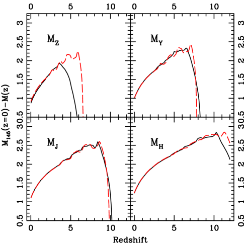
Figure 1: Evolution of $M_{145}(z=0)-M(z)$ in the mock top-hat photometric system (solid lines) and in the UKIDSS photometric system (dashed lines).

We explore a standard color-color selection technique for identifying $z>5$ QSOs. To select objects in the redshift range of interest, we require observations in roughly the $z$ through $H$ or $K$ bands. For illustrative purposes, we consider a representative filter system similar to the one being considered for the DUNE project. This consists of four top-hat filters: a broad optical filter covering the $550$ to $920$ nm interval (roughly corresponding to the $r$, $i$ and $z$ bands; in the following we refer to this filter as $Z$); a $Y$-like filter from $920$ to $1146$ nm; a $J$-like filter from $1146$ to $1372$ nm; and an $H$-like filter from $1372$ to $1800$ nm. This system has the advantage of perfect coverage of the wavelength interval of interest at $5<z<12$, and it gives a good representation of the real filter configurations being considered by the projects we have discussed. In fig. 1 we show the predicted redshift evolution of the difference between the absolute restframe magnitude at 145 nm ($M_{145}$) and the absolute magnitude corresponding to the four filters. We chose $M_{145}$ as a reference magnitude to compare our prediction to the estimate of the QSO LF given in F07. We note that the $\mathit{Ly}_{\alpha}$ line exits each of our four filters at $z=6.57$, $z=8.42$, $z=10.28$ and $z=13.80$ respectively. Given the strong IGM $Ly_{\alpha}$ resonance absorption at $z>6$, for each band these correspond to the redshifts at which the QSOs become “drop-outs”. In the same figure we also plot the predictions of our approach for a more realistic photometric system, namely the UKIDSS ZYJH filter system (dashed line). It is evident from the figure that the response of two photometric systems are in good agreement in the redshift range of interest.

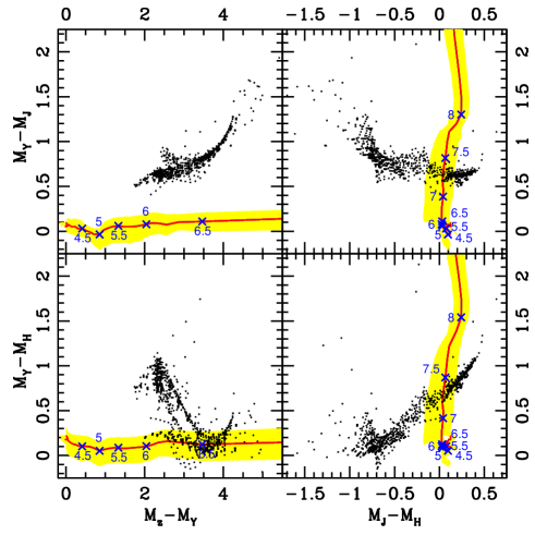
Figure 2: QSO color evolution as a function of redshift in the mock top-hat photometric system. The shaded region represent the scatter in the template library ($5\%$ and $95\%$ percentiles of the distribution). Dots mark the expected colors of brown dwarfs.

We show in fig. 2 four sections of the four dimensional color spaces. The most numerous astrophysical contaminants in dropout searches for high-redshift quasars are cool, low-mass stars (brown dwarfs). The surface density of brown dwarfs at the extremely faint magnitudes considered here is completely unknown and cannot be extrapolated from existing brown-dwarf surveys, though an upper limit is given by the number of dwarf stars in the Milky Way (Wolfgang Brandner, priv. comm.). This is because faint brown dwarfs are the oldest, coolest objects, and their exact magnitude and color distribution depends on the details of the cooling process as well as the distribution of ages and initial masses. For the same reason, it is impossible to quantify the likely number of large-sigma outliers from the mean brown-dwarf locus that would be scattered into the quasar locus. Hence, any brown dwarf sample discovered as by-product of a quasar search would be extremely valuable to the brown-dwarf field. A large fraction of them would be distinguishable from quasars by the $H-K$ color, which is very blue in cold brown dwarfs due to their much higher opacity in the $K$-band than in $H$. We therefore compare our color evolution with the expected colors for brown dwarfs, computed using both the spectral library defined by Reid et al. (2001), and the theoretical spectral model from Burrows et al. (2003,2006) and Hubeny & Burrows (2007). It is evident from fig. 2 that it is possible to define suitable color criteria in order to largely disentangle the two populations. However, since our filter system is only representative, we do not attempt to define quantitative color criteria here. We compare our predictions with simulations and observed colors of quasars in the SDSS and UKIDSS systems (see Chiu et al., 2005, 2007; Hewett et al., 2006); a comparable paper for Pan-STARRS is in preparation (S. Jester, et al. in prep). The good agreement of fig. 2 with, i.e., fig. 11 in Chiu et al. (2005) provides additional evidence that our results are representative, despite the idealized photometric system we assume. We also considered a more standard (narrower) $z$-band instead of the broad-band $Z$ filter. We find that the predicted locus of QSO candidates (yellow shaded region) is not affected by the change; however the narrower filter shows a faster color evolution with respect to fig. 2. The difference is due to the larger $\mathit{Ly}_{\alpha}$ forest flux in the broad-band filter at $z<6$. We therefore conclude that the use of a broader filter allows for a more reliable photometric redshift estimate.

3 Expected QSO counts

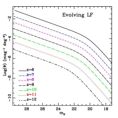
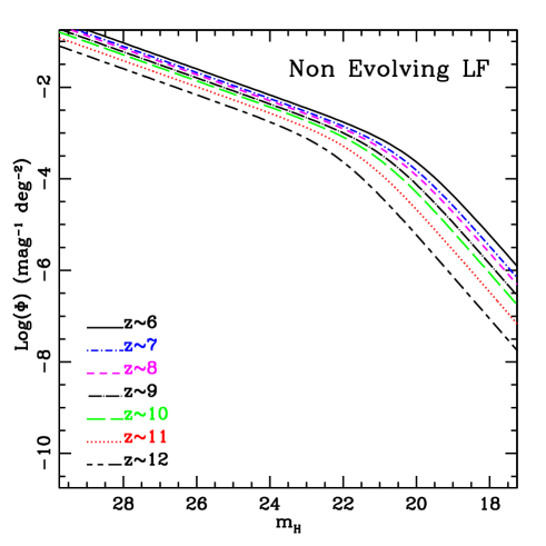
Figure 3: Expected QSO LF evolution in apparent $m_{H}$ magnitude at different redshifts. The left panel shows the non-evolving LF prescription, the right panel the evolving LF prescription, based on the best-fit F07 LF (Nr.13a; see text).

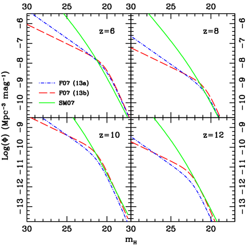
Figure 4: Comparison between the LFs in apparent $m_{H}$ magnitude predicted by the model of F07 (dot-dashed and dashed line refer respectively to model Nr. 13a and Nr. 13b respectively) and SM07 (solid line) models at different redshifts.

3.1 Models for QSO Evolution

Combining our estimate of $M_{145}-m_{H}$ with an estimate of the QSO LF at $z>5$, we can now compute the expected QSO counts in a hypothetical survey as a function of redshift, area and $H$-band depth. We will consider three different models for the evolution of the intrinsic properties of the QSO population: non-evolving luminosity function, evolving luminosity function, and Eddington-limited accretion. In the first model (non-evolving LF), the comoving space density of QSOs is kept fixed to the observed value given by the adopted $z=5$ LF, so that the evolution in the observed population is entirely driven by dimming due to the growing luminosity distance, plus k-corrections. In the second class of models, we make use of the analysis of F07, in which they combined a faint QSO sample obtained from the GOODS survey (Giavalisco et al., 2004), with a bright QSO sample extracted from the SDSSqso3, in order to study the QSO LF and its evolution in the redshift interval $3.5<z<5.2$. They found that Pure Density Evolution models were a better representation of the observed QSO population at these redshifts than Pure Luminosity Evolution models. Their best fit model (Nr. 13a in the original paper) requires an evolution of the magnitude of the knee of the double power law, a relatively steep faint-end slope and a bright-end slope as steep as local observations (in disagreement with Richards et al., 2006; for a discussion of the slope estimates we refer the reader to F07). However, F07 also found a good match between observations and the prediction of a similar model, with a shallower faint-end slope (their model Nr. 13b). These two models roughly correspond to the faint-end slope estimates at lower redshifts given by Richards et al. (2005). Given the importance of the faint-end slope for the prediction of QSO number counts in small area deep surveys, we therefore consider both models in the following discussion.

In fig. 3, we show our assumed LFs, as a function of apparent $m_{H}$, based on the best-fit F07 model (13a), for both the non-evolving and evolving LF. We compare the F07 results with the recent analysis of the QSO-LF at $5<z<6.5$ proposed by Shankar & Mathur (2007, hereafter SM07). They have re-analyzed the SDSS bright sample at $z>5$ (Fan et al., 2001,2004), in the light of recent observations of faint QSOs (Willott et al. 2005; Cool et al. 2006). Their LF has the same double power-law functional form as in F07, while Fan et al. (2004) used a single power law; in order to correctly reproduce the redshift evolution of the SDSS bright sample, SM07 renormalized their LF to the cumulative number density given in Fan et al. (2004) at $z=6.07$, and at each redshift they required the bright-end to match the Fan et al. (2004) LF at $M_{145}=-27.00$ (Shankar, private communication). The SM07 LF has a redshift evolution as in Fan et al. (2001), and a steeper faint-end slope ($<-2.0$) with respect to the F07 results. In the following we consider the 90% CL faint-end slope for the optical LF given in SM07. In fig. 4 we compare the predictions for this model and the two F07 models at different redshift. It is worth noting here that the two groups worked at different redshifts ($3.5<z<5.2$ for F07 and $5.0<z<6.5$ for SM07) and that we are extrapolating their results well beyond these confidence intervals. Keeping these caveats in mind, the overall agreement is quite good.

We compute the number of expected QSO per unit area by integrating the resulting LF up to a limiting magnitude. In order to account for the uncertainties in the evolution of the LF we apply a bootstrap technique. For both F07 models, the redshift evolution is quantified using an exponential form: the authors also give an estimate for the error on this parameter based on their minimization algorithm. Here we consider 1000 Monte Carlo realizations of the expected QSO counts, randomly varying the value of $k_{z}$ over the range of the quoted error. We repeat the procedure for both models for the evolving LF/non-evolving LF and we use the results (mean and variance) to define our predicted range in number counts.

In our third class of models (Eddington), we compute the LF evolution under the hypothesis that the SMBHs responsible for the observed LF at $z\sim 6$ have accreted at the Eddington rate during their entire past history. This gives an exponential mass evolution (see i.e. Volenteri & Rees, 2006):

$$M_{BH}(t)=M_{BH}(0)\exp\big{(}\frac{1-\eta}{\eta}\frac{t}{t_{Edd}}\big{)}$$ (1)

where $t_{Edd}=0.45$ Gyr and $\eta=0.1$ is the radiative efficiency. We convert the mass evolution to luminosity evolution and we predict the corresponding number counts as a function of redshift and depth. We consider both F07 parameterizations (13a and 13b) of the LF as well as the SM07 results and we fixed $z=6$ as the initial redshift for the accretion at the Eddington rate.

3.2 Results

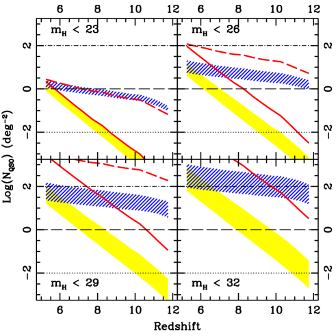
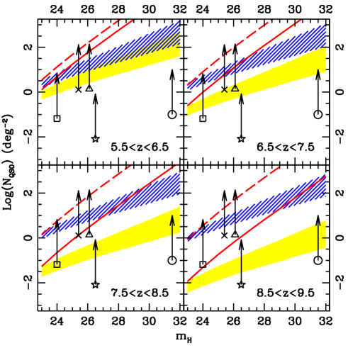
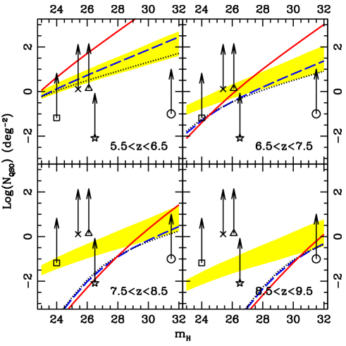
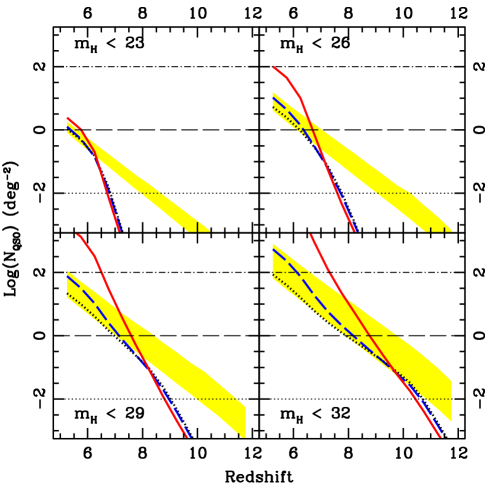
Figure 5: In both panels, the diagonal hatched area shows the predictions of the non-evolving LF model, and the shaded area shows the evolving LF model, both based on the best-fit F07 LF. The shaded regions are estimated via Monte Carlo simulations accounting for the errors in the LF parameters. The solid/dashed line shows the predictions for the evolving/non-evolving LF models based on the SM07 LF. Left Panel: QSO counts as a function of limiting magnitude. The symbols mark the surface density (see also tab. 1) corresponding to one detected QSO in UDS (cross), Ultra-VISTA (triangle), VISTA VIDEO (square), DUNE (star), JWST (circle), while the tip of the arrow shows the surface density that would result in the detection of at least 100 QSOs. Right Panel: QSO counts as a function of redshift. The thin dotted, dashed and dot-dashed horizontal lines mark the levels corresponding to $0.01$, $1$ and $100$ QSO per square degree respectively.

Fig. 5 (left panel) shows the predicted number of QSOs per square degree as a function of limiting magnitude for four redshift intervals ($5.5<z<6.5$, $6.5<z<7.5$, $7.5<z<8.5$, $8.5<z<9.5$). We also show the same quantity as a function of redshift in the right panel. The four panels refer to different magnitude depths ($23.0$, $26.0$, $29.0$, $32.0$). As a reference a $m_{H}=23.00$ magnitude limit corresponds to absolute magnitudes $M_{145}=-23.46$, $-23.73$, $-23.90$ and $-24.16$ at $z=6$, $7$, $8$ and $9$ respectively. We show both the non-evolving and evolving versions of models based on both the F07 LF and the steeper SM07 LF. The difference (several orders of magnitude) at faint magnitudes between the F07-based and the SM07-based models underlines the large uncertainties associated with the faint end of the AGN LF even at lower redshifts, which naturally blow up as we extrapolate these results to higher redshift.

Survey	Depth ($m_{H}$)	Area ($deg^{2}$)
UDS	25.4	0.77
Pan-STARRS Medium Deep Survey	$y<24.8$	80
Pan-STARRS $3\pi$ Survey (extragalactic part)	$y<21.5$	20,000
Ultra-VISTA	26.1	0.73
VISTA VIDEO	24.0	15
SPACE All Sky Survey	23.0	30,000
SPACE Deep Survey	26.0	10
DUNE Medium-Deep	26.5	120
JWST	31.5	10
	Point Source sensitivity	Field of View
	(for 1 Ms observation)	(${\rm arcmin}^{2}$)
XEUS	$3\times 10^{-18}\,{\rm erg/s/cm^{-2}}$	7
Constellation-X	$2\times 10^{-17}\,{\rm erg/s/cm^{-2}}$	5

Table 1: Planned depth and area for the surveys mentioned in the text.

In fig. 5, the symbols show the surface density that would result in the detection of at least one QSO in the UDS, Ultra-Vista, and VISTA-VIDEO surveys at the corresponding $H$-band magnitude depth of the survey, while the tip of the arrow shows the surface density that would result in the detection of at least 100 QSOs. In addition to these already-approved ground-based surveys, we show space-based surveys that could be carried out with the EUCLID and JWST missions. We collect the information about the depth and area of each survey in table 1, where we also list the $y$-band depths of the Pan-STARRS $3\pi$ and Medium Deep Surveys; however since those surveys do not include an $H$-band filter, we do not show them in the plot. For a given magnitude limit and area, the shaded swaths or lines should lie above the arrow tip in order to obtain $>$100 QSOs, or above the symbol in order to detect at least one QSO. One should keep in mind that the diagonal-hatched swaths and dashed lines assume no evolution in the underlying QSO number densities, and are probably overly optimistic. If we take our best-fit F07-based evolving LF model as representative, we see that both the JWST and EUCLID-like surveys are expected to detect a few hundred QSOs in the redshift ranges $6.5<z<7.5$ and $6.5<z<7.5$, and a few tens at $8.5<z<9.5$. However, JWST will mainly constrain the faint end of the QSO LF, while wide-field missions like EUCLID or SNAP are needed to detect significant numbers of bright QSOs.

Fig. 6 shows the prediction of the Eddington accretion model when calibrated to the SM07 and F07 (model Nr.13a and Nr.13b) LFs (see figure caption for model key). To guide the eye, in the same plots we repeat the predictions for the evolving F07 LFs as a shaded area. We can see that the Eddington model predicts much more rapid evolution in the numbers of luminous QSOs, while the predicted numbers of faint objects are within the shaded area of the F07 evolving LF predictions. This illustrates the importance of probing the luminous QSO population for constraining models of BH growth and evolution.

Figure 6: In both panels, the solid, dashed and dotted lines show the predictions for the Eddington accretion models calibrated to the SM07 and F07 (model Nr.13a and Nr.13b) LFs respectively. For comparison, the shaded region reproduces the predictions of the F07-based evolving LF model (as shown in Fig. 5). Symbols and thin lines are as in fig. 5. Left Panel: QSO counts as a function of limiting magnitude. Right Panel: QSO counts as a function of redshift.

We summarize the whole set of predictions for the empirical and semi-empirical models in tab. 2 and tab. 3 respectively.

4 X-ray Surveys

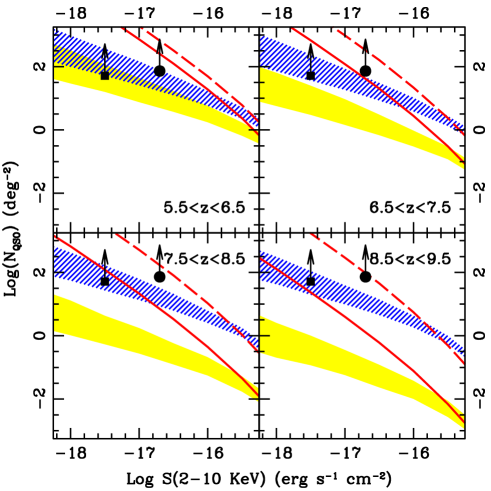
We can use the same approach to estimate the expected number of QSO detected in the hard ($2-10$ keV) X-ray band as a function of redshift, area and flux. We convert the $m_{145}$ magnitudes into X-ray fluxes using the same approach as Fontanot et al. (2006): we compute the bolometric LF using a restframe band correction between $145$ nm and the B-band and the bolometric correction of Elvis et al. (1994); we then convert bolometric into 2-10 keV luminosities following Marconi et al., (2004), and we apply a k-correction in the hard band, calibrated assuming a spectrum with photon index $\Gamma=-1.8$. We do not attempt to correct for the luminosity-dependent fraction of obscured and compton-thick objects. We show the predicted X-ray number counts in fig. 7 corresponding to the same LF models we introduced in 3. In a 1 Ms exposure, XEUS and Con-X are expected to be able to reach a point source sensitivity of $3\times 10^{-18}$ and $2\times 10^{-17}\,{\rm erg/s/cm^{2}}$, respectively (Hasinger et al., 2006). Assuming a maximum total exposure time of 10 Ms, the largest area survey possible with these missions will be about 100 arcmin² (or about $2.8\times 10^{-3}$ sq. deg.). We show the area/depth markings for XEUS and Con-X in fig. 7, as before, except that we show only the symbol that indicates ten AGN per field because the arrow tip would be off the top of the plot. From this we see that blank sky X-ray surveys even with this next generation of missions are unlikely to be an effective means of discovering very high redshift AGN. They may find a few tens to a hundred AGN at $z\sim 6$, but they are unlikely to detect any objects at higher redshift.

Figure 7: Predicted QSO counts in the X-ray 2-10 keV band, for non-evolving and evolving LF models as in Fig. 5. Left Panel: QSO counts as a function of limiting X-ray flux. The symbols mark the expected point source sensitivity and inverse survey area for Constellation-X and XEUS (tab. 1). Right Panel: QSO counts as a function of redshift. We see from this figure that blank sky X-ray surveys with these proposed missions are unlikely to be an effective means of discovering very high redshift AGN.

5 Discussion and Conclusions

In this paper we present empirical predictions of the observed colors and number densities of very high redshift ($z>5$) QSOs. We combine a representative photometric system with a QSO spectral template library to predict the evolution of QSO colors at $z>5$. Using a set of four optical-NIR filters, we show that it is possible to define color-color criteria that select high-z QSO candidates on the basis of their photometric properties. We then combine the estimated k-corrections with different models for the LF evolution in order to estimate the expected number of QSOs as a function of surveyed area, magnitude limit, and redshift.

We confront our findings with the parameters of existing, planned and proposed surveys. First, the SDSS has already covered the bright end of the LF to $M_{145}\approx-26.5$ at $z<6.4$, and is pursuing efforts to push another 2 magnitudes fainter over the 300 square degrees of its deep southern stripe (Jiang et al. 2007). The Pan-STARRS survey, which is about to begin data-taking, will reach $z$ magnitudes that are up to 1 mag fainter still over 20,000 square degrees of extragalactic sky in its $3\pi$ survey, putting of order 3000 low-luminosity quasars at $6<z<6.4$ within its reach (from an extrapolation of the Shankar & Mathur LF). Since the $3\pi$ survey includes deep $z$ and $y$ band imaging, it is also ideally suited for the discovery of quasars at redshifts $6.6\leq z\leq 7.3$. Again integrating the Shankar & Mathur LF to the $y$-band flux limit, we expect that Pan-STARRS will contain of order 150 quasars at $6.6\leq z\leq 7.3$.

In this paper we address the prospects for finding fainter quasars than are accessible with SDSS and Pan-STARRS at $5<z<7.5$, or any quasars at $z>7.5$, with currently planned or proposed surveys. It is evident from fig. 5 that up to $z\la 6.5$, the ground-based near-infrared UKIDSS and VISTA surveys should be able to produce samples of roughly tens to hundreds of low-luminosity QSOs, depending on the actual evolution of the LF. Finding quasars in the Pan-STARRS Medium Deep Survey (MDS) requires complementary near-infrared imaging (ideally in $J$) at the depth of VIDEO (3 of whose fields are included in 3 of the MDS fields); if such imaging is available, the larger area would make about 5-6 times more quasars accessible than VIDEO alone.

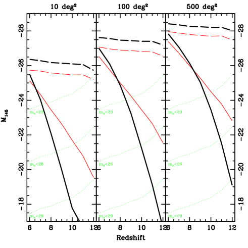
Even in the absence of a decline in the space density of QSOs, however, our results suggest that in order to obtain samples of substantially more than a hundred low-luminosity QSOs at $z\ga 6.5$, we will require the larger survey volumes that are accessible only from space (because of the much lower NIR background, a 2m telescope in space is more efficient at surveying large areas than an 8–10m on the ground). It is also possible to use our predictions to estimate the magnitude of the brightest QSO we expect, as a function of redshift, at a fixed surveyed area (fig. 8). We define this quantity as the magnitude corresponding to an integrated space density of 1 QSO over the surveyed volume (in order to compute the volumes we consider the same redshift intervals as in fig. 5, left panel). We consider the evolving and non-evolving prescriptions (solid and dashed line respectively) applied to the F07a and SM07 LFs (thick and thin line respectively). In the same plot we also show the faintest magnitude reached at a given depth in the $H$-band (dotted lines). Combining the two informations, we are then able to define an accessible magnitude interval.

Figure 8: The magnitude of the brightest QSO in a surveyed area of 10 deg² (left), 100 deg² (middle), 500 deg² (right). Solid and dashed lines correspond to the evolving LF and non-evolving LF prescription respectively. Thick and thin lines correspond to the F07a and SM07 LF respectively. Dotted lines show the faintest absolute limiting magnitude as a function of redshift for a magnitude-limited sample.

Our results highlight that, while JWST will be able to detect extremely faint QSOs, because of its small FOV it is unlikely that it will be possible to survey large enough areas to detect significant numbers of the most luminous QSOs at very high redshift. For this important goal, we need the wider-area surveys that could be carried out by missions like EUCLID or SNAP. Similar arguments hold if we consider planned X-ray surveys with missions such as XEUS and Constellation-X. The very small FOV of these surveys, combined with the relatively long exposure times needed to reach high enough sensitivity, probably preclude the possibility of detecting large samples of $z>6$ QSOs using the X-ray information alone. Targetted X-ray observations of objects detected in the NIR will, however, be crucial for confirming their identity as AGN and constraining obscuration.

The predictions presented here are complementary to those based on semi-analytic models set within the hierarchical structure formation paradigm. For example, Salvaterra, Haardt & Volonteri (2007) have presented predictions for the properties of the AGN population that could be observed in deep X-ray surveys with future surveys, based on the Volonteri & Rees (2006) models with different assumptions. They consider a merger tree based model based on the Press-Schechter formalism and Eddington accretion onto the SMBH. An alternative model has been presented by Rhook & Haehnelt (2008). Their hybrid models also assume that QSO activity is triggered by major merger events, and they combine this information with different sets of assumptions for the decline of the accretion rate onto the SMBH. As in our empirical models, their predicted counts span several orders of magnitude. This underlines the importance of the observational determination of the statistics of the QSO population in order to put constraints on models of SMBH growth. We plan to compare the empirical results presented here with additional semi-analytic, merger-tree based models for SMBH evolution (Fontanot et al. 2007; Somerville et al. 2008) in a forthcoming paper.

We expect that only for the brightest objects will spectroscopic follow-up be feasible. The development of adequate photometric redshift estimators, as well as a larger multi-wavelength coverage, is therefore fundamental for the study of the faint population. Moreover a simple drop-out technique is not able to disentangle a priori faint QSOs from Lyman Break Galaxies at comparable redshift. A key goal in the study of faint high-z QSOs is therefore the definition of reliable criteria to separate QSOs from galaxies. Here, we simply assume that we can perfectly disentangle the faint QSOs from the contaminants such as galaxies and stars. Under this hypothesis we consider a simple test to assess the impact of the uncertainties in the photometric redshift determination on the overall estimate of the QSO-LF and its space density evolution. We consider the F07 Monte Carlo algorithm for the estimate of the LF, which combines the GOODS and SDSS samples. We then introduce a random relative error in the redshifts of the faint (GOODS) objects, perform 1000 bootstrap realizations of LF fitting, and consider the new estimate of the LF parameters. We conclude that the F07 technique is still able to recover the statistical properties of the LF in the presence of these photometric redshift errors: assuming a $5\%$ ($10\%$) error for the photometric redshifts, we add only $0.3\%$ ($0.5\%$) to the error on the redshift evolution and $1.0\%$ ($1.5\%$) to the error on the faint-end slope. Moreover, if we assume a $5\%$ ($10\%$) error on the photometric redshift of all objects (both faint and bright) we add $5\%$ ($10\%$) to the error on the redshift evolution; $10\%$ ($20\%$) to the error on the faint-end slope and $5\%$ ($10\%$) to the error on the bright-end slope.

It seems very likely that at least one “dark energy” mission will fly in the next decade. We have shown here that several of the proposed designs for such missions are also very well-suited to addressing a completely different but important science goal: constraining the formation of massive black holes and luminous QSOs at the earliest epochs in the history of our Universe.

	Non-Evolving LF			Evolving LF			Edd. Accr. LF
	F07a	F07b	SM07	F07a	F07b	SM07	F07a	F07b	SM07
$m_{H}<23$
$5.0<z<5.5$	$1.7$	$1.4$	$2.8$	$1.3$	$1.1$	$2.2$	$1.2$	$1.1$	$2.4$
$5.5<z<6.0$	$1.4$	$1.2$	$2.1$	$0.6$	$0.5$	$1.0$	$0.5$	$0.5$	$1.0$
$6.0<z<6.5$	$1.2$	$1.0$	$1.6$	$0.2$	$0.2$	$0.4$	$0.1$	$0.1$	$0.2$
$6.5<z<7.0$	$1.0$	$0.9$	$1.2$	$0.1$	$0.1$	$0.2$	$1.3\times 10^{-2}$	$1.6\times 10^{-2}$	$7.5\times 10^{-3}$
$7.0<z<7.5$	$0.9$	$0.8$	$1.0$	$4.9\times 10^{-2}$	$4.9\times 10^{-2}$	$8.4\times 10^{-2}$	$5.6\times 10^{-4}$	$6.5\times 10^{-4}$	$3.3\times 10^{-4}$
$7.5<z<8.0$	$0.8$	$0.7$	$0.8$	$2.2\times 10^{-2}$	$2.3\times 10^{-2}$	$3.8\times 10^{-2}$	—	—	—
$8.0<z<8.5$	$0.7$	$0.6$	$0.7$	$1.1\times 10^{-2}$	$1.1\times 10^{-2}$	$2.0\times 10^{-2}$	—	—	—
$8.5<z<9.0$	$0.6$	$0.5$	$0.5$	$4.7\times 10^{-3}$	$5.2\times 10^{-3}$	$8.6\times 10^{-3}$	—	—	—
$9.0<z<9.5$	$0.5$	$0.5$	$0.4$	$2.2\times 10^{-3}$	$2.5\times 10^{-3}$	$4.0\times 10^{-3}$	—	—	—
$9.5<z<10.0$	$0.4$	$0.4$	$0.4$	$9.8\times 10^{-4}$	$1.2\times 10^{-3}$	$1.9\times 10^{-3}$	—	—	—
$10.0<z<10.5$	$0.4$	$0.4$	$0.3$	$4.6\times 10^{-4}$	$5.6\times 10^{-4}$	$9.8\times 10^{-4}$	—	—	—
$10.5<z<11.0$	$0.3$	$0.3$	$0.2$	$1.9\times 10^{-4}$	$2.5\times 10^{-4}$	$3.5\times 10^{-4}$	—	—	—
$11.0<z<11.5$	$0.2$	$0.2$	$0.1$	—	—	$1.2\times 10^{-4}$	—	—	—
$11.5<z<12.0$	$0.1$	$0.1$	$6.7\times 10^{-2}$	—	—	—	—	—	—
$m_{H}<26$
$5.0<z<5.5$	$14.9$	$6.9$	$1.2\times 10^{2}$	$10.9$	$5.3$	$94.3$	$10.3$	$5.3$	$1.0\times 10^{2}$
$5.5<z<6.0$	$12.2$	$6.1$	$92.9$	$4.7$	$2.4$	$42.2$	$4.3$	$2.4$	$43.5$
$6.0<z<6.5$	$10.6$	$5.3$	$74.7$	$2.1$	$1.2$	$19.3$	$1.4$	$0.9$	$10.1$
$6.5<z<7.0$	$9.0$	$4.7$	$58.5$	$1.0$	$0.6$	$8.8$	$0.3$	$0.3$	$0.7$
$7.0<z<7.5$	$7.9$	$4.2$	$47.6$	$0.4$	$0.3$	$4.2$	$6.1\times 10^{-2}$	$7.1\times 10^{-2}$	$5.5\times 10^{-2}$
$7.5<z<8.0$	$7.0$	$3.8$	$39.8$	$0.2$	$0.1$	$2.0$	$8.7\times 10^{-3}$	$1.1\times 10^{-2}$	$4.7\times 10^{-3}$
$8.0<z<8.5$	$6.3$	$3.5$	$36.5$	$9.6\times 10^{-2}$	$6.3\times 10^{-2}$	$1.0$	$9.0\times 10^{-4}$	$1.0\times 10^{-3}$	$5.1\times 10^{-4}$
$8.5<z<9.0$	$5.5$	$3.1$	$28.3$	$4.4\times 10^{-2}$	$3.1\times 10^{-2}$	$0.5$	—	—	—
$9.0<z<9.5$	$4.8$	$2.8$	$23.2$	$2.1\times 10^{-2}$	$1.5\times 10^{-2}$	$0.2$	—	—	—
$9.5<z<10.0$	$4.3$	$2.5$	$20.2$	$9.3\times 10^{-3}$	$7.3\times 10^{-3}$	$0.1$	—	—	—
$10.0<z<10.5$	$3.9$	$2.3$	$18.0$	$5.1\times 10^{-3}$	$3.6\times 10^{-3}$	$5.7\times 10^{-2}$	—	—	—
$10.5<z<11.0$	$3.1$	$1.9$	$12.0$	$2.0\times 10^{-3}$	$1.7\times 10^{-3}$	$2.2\times 10^{-2}$	—	—	—
$11.0<z<11.5$	$2.4$	$1.6$	$7.8$	$8.8\times 10^{-4}$	$7.7\times 10^{-4}$	$8.3\times 10^{-3}$	—	—	—
$11.5<z<12.0$	$1.8$	$1.2$	$5.2$	$3.3\times 10^{-4}$	$3.1\times 10^{-4}$	$3.2\times 10^{-3}$	—	—	—
$m_{H}<29$
$5.0<z<5.5$	$1.1\times 10^{2}$	$28.5$	$3.6\times 10^{3}$	$80.2$	$21.7$	$2.8\times 10^{3}$	$74.9$	$21.6$	$3.0\times 10^{3}$
$5.5<z<6.0$	$90.9$	$25.0$	$2.8\times 10^{3}$	$34.6$	$10.1$	$1.3\times 10^{3}$	$31.6$	$10.0$	$1.3\times 10^{3}$
$6.0<z<6.5$	$75.0$	$22.0$	$2.3\times 10^{3}$	$15.7$	$4.8$	$5.8\times 10^{2}$	$10.3$	$4.0$	$3.2\times 10^{2}$
$6.5<z<7.0$	$66.1$	$19.6$	$1.8\times 10^{3}$	$6.9$	$2.3$	$2.7\times 10^{2}$	$2.6$	$1.5$	$30.3$
$7.0<z<7.5$	$58.2$	$17.7$	$1.5\times 10^{3}$	$3.0$	$1.1$	$1.3\times 10^{2}$	$0.8$	$0.6$	$3.6$
$7.5<z<8.0$	$50.5$	$16.0$	$1.2\times 10^{3}$	$1.5$	$0.5$	$61.0$	$0.2$	$0.2$	$0.5$
$8.0<z<8.5$	$46.4$	$14.8$	$1.1\times 10^{3}$	$0.7$	$0.3$	$32.6$	$7.8\times 10^{-2}$	$8.9\times 10^{-2}$	$7.9\times 10^{-2}$
$8.5<z<9.0$	$40.1$	$13.1$	$9.0\times 10^{2}$	$0.3$	$0.1$	$14.7$	$1.9\times 10^{-2}$	$2.3\times 10^{-2}$	$1.2\times 10^{-2}$
$9.0<z<9.5$	$35.8$	$11.7$	$7.4\times 10^{2}$	$0.2$	$6.5\times 10^{-2}$	$7.1$	$3.7\times 10^{-3}$	$4.5\times 10^{-3}$	$1.9\times 10^{-3}$
$9.5<z<10.0$	$32.5$	$10.7$	$6.5\times 10^{2}$	$7.3\times 10^{-2}$	$3.1\times 10^{-2}$	$3.5$	$6.4\times 10^{-4}$	$7.3\times 10^{-4}$	$3.7\times 10^{-4}$
$10.0<z<10.5$	$28.4$	$9.8$	$5.8\times 10^{2}$	$3.7\times 10^{-2}$	$1.5\times 10^{-2}$	$1.8$	$1.2\times 10^{-4}$	$1.4\times 10^{-4}$	—
$10.5<z<11.0$	$23.7$	$8.4$	$4.0\times 10^{2}$	$1.5\times 10^{-2}$	$7.4\times 10^{-3}$	$0.7$	—	—	—
$11.0<z<11.5$	$18.2$	$6.9$	$2.7\times 10^{2}$	$6.4\times 10^{-3}$	$3.4\times 10^{-3}$	$0.3$	—	—	—
$11.5<z<12.0$	$12.1$	$4.9$	$1.9\times 10^{2}$	$2.6\times 10^{-3}$	$1.4\times 10^{-3}$	$0.1$	—	—	—
$m_{H}<32$
$5.0<z<5.5$	$7.5\times 10^{2}$	$1.1\times 10^{2}$	$9.9\times 10^{4}$	$5.6\times 10^{2}$	$85.2$	$7.8\times 10^{4}$	$5.3\times 10^{2}$	$84.7$	$8.3\times 10^{4}$
$5.5<z<6.0$	$6.3\times 10^{2}$	$98.3$	$7.8\times 10^{4}$	$2.5\times 10^{2}$	$39.6$	$3.5\times 10^{4}$	$2.3\times 10^{2}$	$39.2$	$3.6\times 10^{4}$
$6.0<z<6.5$	$5.4\times 10^{2}$	$86.5$	$6.3\times 10^{4}$	$1.1\times 10^{2}$	$19.0$	$1.6\times 10^{4}$	$74.1$	$16.0$	$8.9\times 10^{3}$
$6.5<z<7.0$	$4.7\times 10^{2}$	$77.1$	$5.0\times 10^{4}$	$49.3$	$9.1$	$7.5\times 10^{3}$	$18.7$	$6.1$	$9.0\times 10^{2}$
$7.0<z<7.5$	$4.0\times 10^{2}$	$69.7$	$4.1\times 10^{4}$	$23.1$	$4.4$	$3.6\times 10^{3}$	$5.8$	$2.6$	$1.2\times 10^{2}$
$7.5<z<8.0$	$3.7\times 10^{2}$	$63.1$	$3.5\times 10^{4}$	$10.6$	$2.1$	$1.7\times 10^{3}$	$2.1$	$1.3$	$22.3$
$8.0<z<8.5$	$3.4\times 10^{2}$	$58.3$	$3.2\times 10^{4}$	$5.3$	$1.1$	$9.1\times 10^{2}$	$0.9$	$0.6$	$4.8$
$8.5<z<9.0$	$2.9\times 10^{2}$	$51.7$	$2.5\times 10^{4}$	$2.4$	$0.5$	$4.1\times 10^{2}$	$0.4$	$0.3$	$1.0$
$9.0<z<9.5$	$2.6\times 10^{2}$	$46.5$	$2.1\times 10^{4}$	$1.1$	$0.3$	$2.0\times 10^{2}$	$0.2$	$0.2$	$0.2$
$9.5<z<10.0$	$2.2\times 10^{2}$	$42.3$	$1.8\times 10^{4}$	$0.5$	$0.1$	$99.6$	$6.4\times 10^{-2}$	$7.4\times 10^{-2}$	$6.0\times 10^{-2}$
$10.0<z<10.5$	$2.1\times 10^{2}$	$39.0$	$1.6\times 10^{4}$	$0.2$	$6.1\times 10^{-2}$	$52.1$	$2.6\times 10^{-2}$	$3.2\times 10^{-2}$	$1.7\times 10^{-2}$
$10.5<z<11.0$	$1.7\times 10^{2}$	$33.4$	$1.1\times 10^{4}$	$0.1$	$2.9\times 10^{-2}$	$21.0$	$7.4\times 10^{-3}$	$9.0\times 10^{-3}$	$3.9\times 10^{-3}$
$11.0<z<11.5$	$1.3\times 10^{2}$	$27.7$	$7.7\times 10^{3}$	$4.6\times 10^{-2}$	$1.4\times 10^{-2}$	$8.1$	$1.5\times 10^{-3}$	$1.7\times 10^{-3}$	$7.9\times 10^{-4}$
$11.5<z<12.0$	$86.7$	$19.4$	$5.4\times 10^{3}$	$1.7\times 10^{-2}$	$5.8\times 10^{-3}$	$3.3$	$2.8\times 10^{-4}$	$3.2\times 10^{-4}$	$1.7\times 10^{-4}$

Table 2: Predicted QSOs counts at different redshift (deg^-2)

	Non-Evolving LF			Evolving LF			Edd. Accr. LF
	F07a	F07b	SM07	F07a	F07b	SM07	F07a	F07b	SM07
$5.5<z<6.5$
$m_{H}<23.0$	$2.4$	$2.0$	$3.4$	$0.7$	$0.7$	$1.3$	$0.6$	$0.6$	$1.1$
$m_{H}<24.0$	$5.2$	$3.7$	$13.3$	$1.6$	$1.2$	$4.9$	$1.3$	$1.1$	$4.2$
$m_{H}<25.0$	$10.7$	$6.4$	$46.9$	$3.2$	$2.0$	$17.3$	$2.7$	$1.9$	$14.9$
$m_{H}<26.0$	$21.3$	$10.6$	$1.5\times 10^{2}$	$6.3$	$3.4$	$57.2$	$5.3$	$3.1$	$49.2$
$m_{H}<27.0$	$39.9$	$16.8$	$4.9\times 10^{2}$	$12.5$	$5.5$	$1.8\times 10^{2}$	$10.3$	$5.0$	$1.6\times 10^{2}$
$m_{H}<28.0$	$78.6$	$27.2$	$1.5\times 10^{3}$	$23.8$	$8.7$	$5.6\times 10^{2}$	$20.0$	$8.1$	$4.8\times 10^{2}$
$m_{H}<29.0$	$1.5\times 10^{2}$	$42.8$	$4.7\times 10^{3}$	$45.2$	$13.7$	$1.7\times 10^{3}$	$38.7$	$12.9$	$1.5\times 10^{3}$
$m_{H}<30.0$	$2.9\times 10^{2}$	$68.2$	$1.4\times 10^{4}$	$89.2$	$22.0$	$5.2\times 10^{3}$	$74.6$	$20.5$	$4.5\times 10^{3}$
$m_{H}<31.0$	$5.7\times 10^{2}$	$1.1\times 10^{2}$	$4.3\times 10^{4}$	$1.7\times 10^{2}$	$34.8$	$1.6\times 10^{4}$	$1.4\times 10^{2}$	$32.3$	$1.4\times 10^{4}$
$m_{H}<32.0$	$1.1\times 10^{3}$	$1.7\times 10^{2}$	$1.3\times 10^{5}$	$3.3\times 10^{2}$	$54.7$	$4.8\times 10^{4}$	$2.8\times 10^{2}$	$50.9$	$4.1\times 10^{4}$
$6.5<z<7.5$
$m_{H}<23.0$	$1.8$	$1.5$	$2.0$	$0.1$	$0.1$	$0.2$	$1.3\times 10^{-2}$	$1.6\times 10^{-2}$	$7.7\times 10^{-3}$
$m_{H}<24.0$	$3.9$	$2.8$	$8.0$	$0.3$	$0.3$	$1.0$	$4.9\times 10^{-2}$	$5.8\times 10^{-2}$	$4.0\times 10^{-2}$
$m_{H}<25.0$	$7.7$	$5.0$	$28.8$	$0.6$	$0.5$	$3.6$	$0.1$	$0.2$	$0.2$
$m_{H}<26.0$	$15.2$	$8.3$	$97.0$	$1.3$	$0.8$	$11.9$	$0.3$	$0.3$	$0.8$
$m_{H}<27.0$	$30.1$	$13.2$	$3.1\times 10^{2}$	$2.5$	$1.2$	$38.3$	$0.8$	$0.6$	$2.9$
$m_{H}<28.0$	$59.5$	$21.4$	$9.7\times 10^{2}$	$4.9$	$2.0$	$1.2\times 10^{2}$	$1.6$	$1.1$	$9.9$
$m_{H}<29.0$	$1.1\times 10^{2}$	$33.8$	$3.0\times 10^{3}$	$9.2$	$3.1$	$3.7\times 10^{2}$	$3.1$	$1.9$	$32.6$
$m_{H}<30.0$	$2.2\times 10^{2}$	$53.8$	$9.1\times 10^{3}$	$18.3$	$5.0$	$1.1\times 10^{3}$	$6.1$	$3.1$	$1.0\times 10^{2}$
$m_{H}<31.0$	$4.2\times 10^{2}$	$85.9$	$2.8\times 10^{4}$	$36.8$	$8.0$	$3.4\times 10^{3}$	$11.9$	$5.1$	$3.2\times 10^{2}$
$m_{H}<32.0$	$8.1\times 10^{2}$	$1.3\times 10^{2}$	$8.3\times 10^{4}$	$69.1$	$12.5$	$1.0\times 10^{4}$	$23.0$	$8.1$	$9.8\times 10^{2}$
$7.5<z<8.5$
$m_{H}<23.0$	$1.3$	$1.2$	$1.4$	$3.0\times 10^{-2}$	$3.2\times 10^{-2}$	$5.4\times 10^{-2}$	—	—	—
$m_{H}<24.0$	$2.9$	$2.3$	$5.6$	$6.6\times 10^{-2}$	$6.0\times 10^{-2}$	$0.2$	$2.0\times 10^{-4}$	$2.3\times 10^{-4}$	$1.3\times 10^{-4}$
$m_{H}<25.0$	$5.9$	$4.0$	$20.5$	$0.1$	$0.1$	$0.8$	$1.6\times 10^{-3}$	$1.8\times 10^{-3}$	$8.6\times 10^{-4}$
$m_{H}<26.0$	$12.0$	$6.8$	$69.8$	$0.3$	$0.2$	$2.8$	$9.2\times 10^{-3}$	$1.1\times 10^{-2}$	$5.0\times 10^{-3}$
$m_{H}<27.0$	$23.5$	$10.8$	$2.3\times 10^{2}$	$0.5$	$0.3$	$9.0$	$3.9\times 10^{-2}$	$4.7\times 10^{-2}$	$2.7\times 10^{-2}$
$m_{H}<28.0$	$45.1$	$17.6$	$7.1\times 10^{2}$	$1.0$	$0.5$	$28.0$	$0.1$	$0.1$	$0.1$
$m_{H}<29.0$	$88.5$	$27.8$	$2.2\times 10^{3}$	$2.0$	$0.7$	$86.3$	$0.3$	$0.3$	$0.6$
$m_{H}<30.0$	$1.7\times 10^{2}$	$44.3$	$6.6\times 10^{3}$	$3.7$	$1.2$	$2.6\times 10^{2}$	$0.7$	$0.6$	$2.2$
$m_{H}<31.0$	$3.4\times 10^{2}$	$70.8$	$2.0\times 10^{4}$	$7.3$	$1.9$	$8.0\times 10^{2}$	$1.4$	$1.0$	$7.7$
$m_{H}<32.0$	$6.3\times 10^{2}$	$1.1\times 10^{2}$	$6.1\times 10^{4}$	$14.1$	$3.0$	$2.4\times 10^{3}$	$2.8$	$1.7$	$25.6$
$8.5<z<9.5$
$m_{H}<23.0$	$0.9$	$0.9$	$0.9$	$6.2\times 10^{-3}$	$7.1\times 10^{-3}$	$1.2\times 10^{-2}$	—	—	—
$m_{H}<24.0$	$2.2$	$1.8$	$3.6$	$1.4\times 10^{-2}$	$1.4\times 10^{-2}$	$4.9\times 10^{-2}$	—	—	—
$m_{H}<25.0$	$4.7$	$3.2$	$13.6$	$3.0\times 10^{-2}$	$2.5\times 10^{-2}$	$0.2$	—	—	—
$m_{H}<26.0$	$9.5$	$5.4$	$46.9$	$5.9\times 10^{-2}$	$4.2\times 10^{-2}$	$0.6$	—	—	—
$m_{H}<27.0$	$18.0$	$8.7$	$1.5\times 10^{2}$	$0.1$	$7.0\times 10^{-2}$	$2.1$	$6.4\times 10^{-4}$	$7.4\times 10^{-4}$	$3.8\times 10^{-4}$
$m_{H}<28.0$	$35.6$	$14.2$	$4.8\times 10^{2}$	$0.2$	$0.1$	$6.5$	$4.4\times 10^{-3}$	$5.2\times 10^{-3}$	$2.3\times 10^{-3}$
$m_{H}<29.0$	$67.7$	$22.5$	$1.5\times 10^{3}$	$0.4$	$0.2$	$20.0$	$2.2\times 10^{-2}$	$2.6\times 10^{-2}$	$1.3\times 10^{-2}$
$m_{H}<30.0$	$1.3\times 10^{2}$	$35.9$	$4.6\times 10^{3}$	$0.9$	$0.3$	$61.1$	$7.6\times 10^{-2}$	$8.9\times 10^{-2}$	$6.5\times 10^{-2}$
$m_{H}<31.0$	$2.6\times 10^{2}$	$57.4$	$1.4\times 10^{4}$	$1.7$	$0.5$	$1.9\times 10^{2}$	$0.2$	$0.2$	$0.3$
$m_{H}<32.0$	$4.9\times 10^{2}$	$90.0$	$4.2\times 10^{4}$	$3.2$	$0.7$	$5.6\times 10^{2}$	$0.5$	$0.4$	$1.2$

Table 3: Predicted QSOs counts at different $H$-band limits (deg^-2)

	Non-Evolving LF			Evolving LF			Edd. Accr. LF
	F07a	F07b	SM07	F07a	F07b	SM07	F07a	F07b	SM07
$S(2-10KeV)<10^{-15.5}erg/s/cm^{-2}$
$5.0<z<5.5$	$3.0$	$1.7$	$6.6$	$2.1$	$1.2$	$5.3$	$2.0$	$1.6$	$5.8$
$5.5<z<6.0$	$2.3$	$1.3$	$4.0$	$0.9$	$0.5$	$1.8$	$0.8$	$0.7$	$2.1$
$6.0<z<6.5$	$1.7$	$1.0$	$2.5$	$0.3$	$0.2$	$0.7$	$0.2$	$0.2$	$0.4$
$6.5<z<7.0$	$1.2$	$0.7$	$1.6$	$0.1$	$8.8\times 10^{-2}$	$0.2$	$1.8\times 10^{-2}$	$2.2\times 10^{-2}$	$1.1\times 10^{-2}$
$7.0<z<7.5$	$1.0$	$0.6$	$1.0$	$5.7\times 10^{-2}$	$3.9\times 10^{-2}$	$8.8\times 10^{-2}$	$7.2\times 10^{-4}$	$8.3\times 10^{-4}$	$4.1\times 10^{-4}$
$7.5<z<8.0$	$0.7$	$0.5$	$0.7$	$2.2\times 10^{-2}$	$1.6\times 10^{-2}$	$3.4\times 10^{-2}$	—	—	—
$8.0<z<8.5$	$0.6$	$0.4$	$0.5$	$9.7\times 10^{-3}$	$7.1\times 10^{-3}$	$1.4\times 10^{-2}$	—	—	—
$8.5<z<9.0$	$0.5$	$0.3$	$0.3$	$4.1\times 10^{-3}$	$3.0\times 10^{-3}$	$5.4\times 10^{-3}$	—	—	—
$9.0<z<9.5$	$0.4$	$0.2$	$0.2$	$1.5\times 10^{-3}$	$1.2\times 10^{-3}$	$2.2\times 10^{-3}$	—	—	—
$9.5<z<10.0$	$0.3$	$0.2$	$0.2$	$7.7\times 10^{-4}$	$5.6\times 10^{-4}$	$9.2\times 10^{-4}$	—	—	—
$10.0<z<10.5$	$0.2$	$0.1$	$0.1$	$3.2\times 10^{-4}$	$2.3\times 10^{-4}$	$3.7\times 10^{-4}$	—	—	—
$10.5<z<11.0$	$0.2$	$0.1$	$8.4\times 10^{-2}$	$1.2\times 10^{-4}$	—	$1.5\times 10^{-4}$	—	—	—
$11.0<z<11.5$	$0.1$	$8.2\times 10^{-2}$	$6.1\times 10^{-2}$	—	—	—	—	—	—
$11.5<z<12.0$	$0.1$	$6.1\times 10^{-2}$	$4.4\times 10^{-2}$	—	—	—	—	—	—
$S(2-10KeV)<10^{-16.5}erg/s/cm^{-2}$
$5.0<z<5.5$	$27.3$	$11.2$	$3.3\times 10^{2}$	$20.8$	$8.6$	$2.6\times 10^{2}$	$18.6$	$8.1$	$2.9\times 10^{2}$
$5.5<z<6.0$	$22.3$	$9.5$	$2.1\times 10^{2}$	$8.0$	$3.7$	$96.7$	$7.2$	$3.5$	$1.1\times 10^{2}$
$6.0<z<6.5$	$16.7$	$7.7$	$1.4\times 10^{2}$	$3.8$	$1.8$	$36.7$	$2.1$	$1.3$	$22.8$
$6.5<z<7.0$	$13.6$	$6.4$	$1.0\times 10^{2}$	$1.2$	$0.7$	$15.4$	$0.4$	$0.4$	$1.4$
$7.0<z<7.5$	$11.2$	$5.5$	$73.2$	$0.6$	$0.3$	$6.4$	$9.0\times 10^{-2}$	$0.1$	$10.0\times 10^{-2}$
$7.5<z<8.0$	$9.1$	$4.7$	$51.0$	$0.3$	$0.2$	$2.6$	$1.3\times 10^{-2}$	$1.6\times 10^{-2}$	$7.2\times 10^{-3}$
$8.0<z<8.5$	$7.2$	$3.9$	$36.5$	$9.8\times 10^{-2}$	$6.8\times 10^{-2}$	$1.0$	$1.1\times 10^{-3}$	$1.3\times 10^{-3}$	$6.0\times 10^{-4}$
$8.5<z<9.0$	$5.7$	$3.3$	$27.3$	$5.2\times 10^{-2}$	$3.5\times 10^{-2}$	$0.5$	—	—	—
$9.0<z<9.5$	$5.0$	$2.9$	$21.2$	$2.4\times 10^{-2}$	$1.7\times 10^{-2}$	$0.2$	—	—	—
$9.5<z<10.0$	$3.9$	$2.4$	$16.6$	$1.0\times 10^{-2}$	$7.5\times 10^{-3}$	$9.1\times 10^{-2}$	—	—	—
$10.0<z<10.5$	$3.6$	$2.2$	$12.4$	$4.0\times 10^{-3}$	$3.4\times 10^{-3}$	$3.9\times 10^{-2}$	—	—	—
$10.5<z<11.0$	$2.8$	$1.8$	$9.7$	$1.8\times 10^{-3}$	$1.5\times 10^{-3}$	$1.8\times 10^{-2}$	—	—	—
$11.0<z<11.5$	$2.7$	$1.7$	$7.5$	$9.6\times 10^{-4}$	$8.1\times 10^{-4}$	$8.0\times 10^{-3}$	—	—	—
$11.5<z<12.0$	$2.2$	$1.5$	$6.1$	$4.4\times 10^{-4}$	$3.9\times 10^{-4}$	$3.7\times 10^{-3}$	—	—	—
$S(2-10KeV)<10^{-17.5}erg/s/cm^{-2}$
$5.0<z<5.5$	$2.2\times 10^{2}$	$48.8$	$1.0\times 10^{4}$	$1.6\times 10^{2}$	$35.9$	$8.0\times 10^{3}$	$1.4\times 10^{2}$	$33.2$	$8.4\times 10^{3}$
$5.5<z<6.0$	$1.6\times 10^{2}$	$38.1$	$6.6\times 10^{3}$	$62.3$	$15.7$	$3.0\times 10^{3}$	$54.4$	$14.6$	$3.3\times 10^{3}$
$6.0<z<6.5$	$1.2\times 10^{2}$	$30.7$	$4.8\times 10^{3}$	$26.4$	$7.2$	$1.3\times 10^{3}$	$16.5$	$5.6$	$7.3\times 10^{2}$
$6.5<z<7.0$	$1.1\times 10^{2}$	$27.8$	$3.4\times 10^{3}$	$11.8$	$3.4$	$5.1\times 10^{2}$	$3.8$	$2.0$	$60.9$
$7.0<z<7.5$	$88.9$	$24.2$	$2.4\times 10^{3}$	$4.3$	$1.4$	$2.1\times 10^{2}$	$1.1$	$0.8$	$6.7$
$7.5<z<8.0$	$72.0$	$20.5$	$1.8\times 10^{3}$	$1.8$	$0.6$	$90.5$	$0.3$	$0.3$	$0.8$
$8.0<z<8.5$	$59.9$	$17.7$	$1.4\times 10^{3}$	$0.9$	$0.3$	$39.7$	$9.7\times 10^{-2}$	$0.1$	$0.1$
$8.5<z<9.0$	$48.0$	$15.1$	$1.0\times 10^{3}$	$0.4$	$0.1$	$17.4$	$2.4\times 10^{-2}$	$2.9\times 10^{-2}$	$1.5\times 10^{-2}$
$9.0<z<9.5$	$39.5$	$13.0$	$8.3\times 10^{2}$	$0.2$	$7.7\times 10^{-2}$	$7.9$	$4.6\times 10^{-3}$	$5.5\times 10^{-3}$	$2.4\times 10^{-3}$
$9.5<z<10.0$	$35.8$	$11.9$	$6.5\times 10^{2}$	$8.5\times 10^{-2}$	$3.5\times 10^{-2}$	$3.5$	$7.0\times 10^{-4}$	$8.1\times 10^{-4}$	$4.0\times 10^{-4}$
$10.0<z<10.5$	$30.1$	$10.4$	$5.2\times 10^{2}$	$3.3\times 10^{-2}$	$1.6\times 10^{-2}$	$1.6$	$1.1\times 10^{-4}$	$1.2\times 10^{-4}$	—
$10.5<z<11.0$	$25.8$	$9.2$	$4.1\times 10^{2}$	$1.5\times 10^{-2}$	$7.6\times 10^{-3}$	$0.8$	—	—	—
$11.0<z<11.5$	$21.9$	$8.1$	$3.3\times 10^{2}$	$7.8\times 10^{-3}$	$3.8\times 10^{-3}$	$0.3$	—	—	—
$11.5<z<12.0$	$19.7$	$7.4$	$2.7\times 10^{2}$	$3.5\times 10^{-3}$	$1.8\times 10^{-3}$	$0.2$	—	—	—
$S(2-10KeV)<10^{-18.5}erg/s/cm^{-2}$
$5.0<z<5.5$	$1.4\times 10^{3}$	$1.7\times 10^{2}$	$2.4\times 10^{5}$	$1.1\times 10^{3}$	$1.4\times 10^{2}$	$1.9\times 10^{5}$	$9.0\times 10^{2}$	$1.2\times 10^{2}$	$2.0\times 10^{5}$
$5.5<z<6.0$	$1.1\times 10^{3}$	$1.4\times 10^{2}$	$1.6\times 10^{5}$	$4.3\times 10^{2}$	$59.8$	$7.5\times 10^{4}$	$3.6\times 10^{2}$	$54.1$	$8.2\times 10^{4}$
$6.0<z<6.5$	$7.9\times 10^{2}$	$1.2\times 10^{2}$	$1.2\times 10^{5}$	$1.9\times 10^{2}$	$28.2$	$3.0\times 10^{4}$	$1.1\times 10^{2}$	$21.1$	$1.9\times 10^{4}$
$6.5<z<7.0$	$6.7\times 10^{2}$	$1.0\times 10^{2}$	$8.4\times 10^{4}$	$68.9$	$11.7$	$1.3\times 10^{4}$	$26.0$	$7.6$	$1.6\times 10^{3}$
$7.0<z<7.5$	$5.6\times 10^{2}$	$87.9$	$6.4\times 10^{4}$	$31.8$	$5.7$	$5.6\times 10^{3}$	$7.6$	$3.2$	$2.0\times 10^{2}$
$7.5<z<8.0$	$4.7\times 10^{2}$	$76.4$	$4.9\times 10^{4}$	$15.0$	$2.8$	$2.4\times 10^{3}$	$2.6$	$1.5$	$32.4$
$8.0<z<8.5$	$4.1\times 10^{2}$	$68.3$	$3.7\times 10^{4}$	$6.2$	$1.3$	$1.1\times 10^{3}$	$1.0$	$0.7$	$6.1$
$8.5<z<9.0$	$3.4\times 10^{2}$	$58.8$	$2.9\times 10^{4}$	$2.8$	$0.6$	$4.9\times 10^{2}$	$0.4$	$0.3$	$1.3$
$9.0<z<9.5$	$2.8\times 10^{2}$	$51.6$	$2.2\times 10^{4}$	$1.3$	$0.3$	$2.1\times 10^{2}$	$0.2$	$0.2$	$0.3$
$9.5<z<10.0$	$2.6\times 10^{2}$	$47.0$	$1.8\times 10^{4}$	$0.6$	$0.1$	$99.6$	$6.6\times 10^{-2}$	$7.6\times 10^{-2}$	$6.4\times 10^{-2}$
$10.0<z<10.5$	$2.2\times 10^{2}$	$42.0$	$1.5\times 10^{4}$	$0.3$	$6.6\times 10^{-2}$	$46.4$	$2.4\times 10^{-2}$	$2.9\times 10^{-2}$	$1.6\times 10^{-2}$
$10.5<z<11.0$	$1.9\times 10^{2}$	$37.2$	$1.2\times 10^{4}$	$0.1$	$3.1\times 10^{-2}$	$21.4$	$7.7\times 10^{-3}$	$9.4\times 10^{-3}$	$4.1\times 10^{-3}$
$11.0<z<11.5$	$1.6\times 10^{2}$	$32.7$	$9.7\times 10^{3}$	$6.5\times 10^{-2}$	$1.6\times 10^{-2}$	$10.2$	$2.2\times 10^{-3}$	$2.6\times 10^{-3}$	$1.1\times 10^{-3}$
$11.5<z<12.0$	$1.3\times 10^{2}$	$29.1$	$8.0\times 10^{3}$	$2.6\times 10^{-2}$	$7.5\times 10^{-3}$	$4.7$	$6.0\times 10^{-4}$	$7.0\times 10^{-4}$	$3.5\times 10^{-4}$

Table 4: Predicted QSOs counts at different redshift (deg^-2)

	Non-Evolving LF			Evolving LF			Edd. Accr. LF
	F07a	F07b	SM07	F07a	F07b	SM07	F07a	F07b	SM07
$5.5<z<6.5$
$log(S)<-14.0$	$4.2\times 10^{-3}$	$3.9\times 10^{-3}$	$1.4\times 10^{-3}$	$1.3\times 10^{-3}$	$1.3\times 10^{-3}$	$5.6\times 10^{-4}$	$1.1\times 10^{-3}$	$1.2\times 10^{-3}$	$6.1\times 10^{-4}$
$log(S)<-14.5$	$9.3\times 10^{-2}$	$9.9\times 10^{-2}$	$3.2\times 10^{-2}$	$3.0\times 10^{-2}$	$3.4\times 10^{-2}$	$1.3\times 10^{-2}$	$2.6\times 10^{-2}$	$3.0\times 10^{-2}$	$1.3\times 10^{-2}$
$log(S)<-15.0$	$0.8$	$0.8$	$0.5$	$0.3$	$0.3$	$0.2$	$0.2$	$0.2$	$0.2$
$log(S)<-15.5$	$3.7$	$2.9$	$6.0$	$1.1$	$0.9$	$2.3$	$0.9$	$0.8$	$2.2$
$log(S)<-16.0$	$12.4$	$7.2$	$49.2$	$4.0$	$2.4$	$19.0$	$2.9$	$2.0$	$17.9$
$log(S)<-16.5$	$36.3$	$15.8$	$3.3\times 10^{2}$	$11.3$	$5.2$	$1.2\times 10^{2}$	$8.6$	$4.4$	$1.2\times 10^{2}$
$log(S)<-17.0$	$1.0\times 10^{2}$	$33.2$	$1.9\times 10^{3}$	$29.3$	$10.3$	$7.3\times 10^{2}$	$24.2$	$9.2$	$6.9\times 10^{2}$
$log(S)<-17.5$	$2.7\times 10^{2}$	$65.4$	$1.0\times 10^{4}$	$80.3$	$21.0$	$3.9\times 10^{3}$	$65.5$	$18.6$	$3.8\times 10^{3}$
$log(S)<-18.0$	$6.8\times 10^{2}$	$1.3\times 10^{2}$	$5.4\times 10^{4}$	$2.2\times 10^{2}$	$41.4$	$2.1\times 10^{4}$	$1.7\times 10^{2}$	$36.4$	$1.9\times 10^{4}$
$log(S)<-18.5$	$1.8\times 10^{3}$	$2.5\times 10^{2}$	$2.6\times 10^{5}$	$5.4\times 10^{2}$	$78.7$	$9.8\times 10^{4}$	$4.3\times 10^{2}$	$69.4$	$9.2\times 10^{4}$
$6.5<z<7.5$
$log(S)<-14.0$	$1.1\times 10^{-3}$	$1.0\times 10^{-3}$	$4.1\times 10^{-4}$	—	$1.0\times 10^{-4}$	—	—	—	—
$log(S)<-14.5$	$3.0\times 10^{-2}$	$3.1\times 10^{-2}$	$1.0\times 10^{-2}$	$2.9\times 10^{-3}$	$3.3\times 10^{-3}$	$1.3\times 10^{-3}$	—	—	—
$log(S)<-15.0$	$0.4$	$0.4$	$0.2$	$3.5\times 10^{-2}$	$4.1\times 10^{-2}$	$2.4\times 10^{-2}$	$1.1\times 10^{-3}$	$1.3\times 10^{-3}$	$6.2\times 10^{-4}$
$log(S)<-15.5$	$1.9$	$1.7$	$2.4$	$0.2$	$0.2$	$0.3$	$1.8\times 10^{-2}$	$2.2\times 10^{-2}$	$1.1\times 10^{-2}$
$log(S)<-16.0$	$7.6$	$4.8$	$21.8$	$0.6$	$0.4$	$2.8$	$0.1$	$0.1$	$0.2$
$log(S)<-16.5$	$21.9$	$10.7$	$1.6\times 10^{2}$	$1.9$	$1.0$	$20.1$	$0.5$	$0.5$	$1.5$
$log(S)<-17.0$	$63.0$	$23.0$	$9.6\times 10^{2}$	$5.7$	$2.2$	$1.2\times 10^{2}$	$1.6$	$1.1$	$10.5$
$log(S)<-17.5$	$1.7\times 10^{2}$	$46.3$	$5.3\times 10^{3}$	$15.5$	$4.5$	$6.7\times 10^{2}$	$4.6$	$2.5$	$65.1$
$log(S)<-18.0$	$4.6\times 10^{2}$	$92.6$	$2.8\times 10^{4}$	$39.5$	$8.8$	$3.6\times 10^{3}$	$12.3$	$5.2$	$3.5\times 10^{2}$
$log(S)<-18.5$	$1.2\times 10^{3}$	$1.8\times 10^{2}$	$1.4\times 10^{5}$	$93.3$	$16.3$	$1.7\times 10^{4}$	$31.6$	$10.1$	$1.7\times 10^{3}$
$7.5<z<8.5$
$log(S)<-14.0$	$3.5\times 10^{-4}$	$3.2\times 10^{-4}$	$1.2\times 10^{-4}$	—	—	—	—	—	—
$log(S)<-14.5$	$1.0\times 10^{-2}$	$1.0\times 10^{-2}$	$3.7\times 10^{-3}$	$2.6\times 10^{-4}$	$3.2\times 10^{-4}$	$1.6\times 10^{-4}$	—	—	—
$log(S)<-15.0$	$0.2$	$0.2$	$7.6\times 10^{-2}$	$5.1\times 10^{-3}$	$6.2\times 10^{-3}$	$3.3\times 10^{-3}$	—	—	—
$log(S)<-15.5$	$1.3$	$1.2$	$1.1$	$2.9\times 10^{-2}$	$3.1\times 10^{-2}$	$4.5\times 10^{-2}$	—	—	—
$log(S)<-16.0$	$4.4$	$3.2$	$10.6$	$0.1$	$9.6\times 10^{-2}$	$0.4$	$7.5\times 10^{-4}$	$8.7\times 10^{-4}$	$4.3\times 10^{-4}$
$log(S)<-16.5$	$15.2$	$7.9$	$81.0$	$0.3$	$0.2$	$3.4$	$1.3\times 10^{-2}$	$1.6\times 10^{-2}$	$7.6\times 10^{-3}$
$log(S)<-17.0$	$44.2$	$17.2$	$5.2\times 10^{2}$	$1.0$	$0.5$	$21.5$	$9.7\times 10^{-2}$	$0.1$	$9.9\times 10^{-2}$
$log(S)<-17.5$	$1.2\times 10^{2}$	$34.7$	$2.9\times 10^{3}$	$2.5$	$0.9$	$1.2\times 10^{2}$	$0.4$	$0.4$	$0.9$
$log(S)<-18.0$	$3.1\times 10^{2}$	$68.6$	$1.6\times 10^{4}$	$7.2$	$1.8$	$6.6\times 10^{2}$	$1.2$	$0.9$	$6.4$
$log(S)<-18.5$	$7.7\times 10^{2}$	$1.3\times 10^{2}$	$7.9\times 10^{4}$	$17.5$	$3.5$	$3.3\times 10^{3}$	$3.4$	$2.0$	$36.6$
$8.5<z<9.5$
$log(S)<-14.0$	$1.2\times 10^{-4}$	$1.1\times 10^{-4}$	—	—	—	—	—	—	—
$log(S)<-14.5$	$4.2\times 10^{-3}$	$4.1\times 10^{-3}$	$1.5\times 10^{-3}$	—	—	—	—	—	—
$log(S)<-15.0$	$9.9\times 10^{-2}$	$0.1$	$3.1\times 10^{-2}$	$6.0\times 10^{-4}$	$8.2\times 10^{-4}$	$4.3\times 10^{-4}$	—	—	—
$log(S)<-15.5$	$0.7$	$0.7$	$0.5$	$4.6\times 10^{-3}$	$5.6\times 10^{-3}$	$7.0\times 10^{-3}$	—	—	—
$log(S)<-16.0$	$3.1$	$2.3$	$5.5$	$2.1\times 10^{-2}$	$1.9\times 10^{-2}$	$7.7\times 10^{-2}$	—	—	—
$log(S)<-16.5$	$10.1$	$5.7$	$44.9$	$6.4\times 10^{-2}$	$4.5\times 10^{-2}$	$0.6$	—	—	—
$log(S)<-17.0$	$28.4$	$12.4$	$2.9\times 10^{2}$	$0.2$	$0.1$	$4.0$	$2.2\times 10^{-3}$	$2.6\times 10^{-3}$	$1.2\times 10^{-3}$
$log(S)<-17.5$	$77.7$	$25.3$	$1.7\times 10^{3}$	$0.6$	$0.2$	$23.5$	$2.7\times 10^{-2}$	$3.3\times 10^{-2}$	$1.7\times 10^{-2}$
$log(S)<-18.0$	$2.3\times 10^{2}$	$53.6$	$9.3\times 10^{3}$	$1.3$	$0.4$	$1.3\times 10^{2}$	$0.2$	$0.2$	$0.2$
$log(S)<-18.5$	$5.6\times 10^{2}$	$1.0\times 10^{2}$	$4.8\times 10^{4}$	$4.2$	$0.9$	$6.5\times 10^{2}$	$0.5$	$0.5$	$1.5$

Table 5: Predicted QSOs counts at different X-ray flux limits (deg^-2)

References

• [1] Bower, R. G., Benson, A. J., Malbon, R., et al. 2006, MNRAS, 370, 645
• [2] Bromley, J.Β M., Somerville, R.Β S., & Fabian, A.Β C.Β 2004, MNRAS, 350, 456
• [3] Burrows, A., Sudarsky, D., & Lunine, J.Β I.Β 2003, ApJ, 596, 587
• [4] Burrows, A., Sudarsky, D., & Hubeny, I.Β 2006, ApJ, 640, 1063
• [5] Chiu, K., et al.Β 2005, AJ, 130, 13
• [6] Chiu, K., Richards, G.Β T., Hewett, P.Β C., & Maddox, N.Β 2007, MNRAS, 375, 1180
• [7] Croom S. M., Smith R. J., Boyle B. J., Shanks T., Miller L., Outram P. J., Loaring N. S., 2004, MNRAS, 349, 1397
• [8] Croton, D. J., Springel, V., White, S. D. M., et al. 2006, MNRAS, 365, 11
• [9] Elvis, M., et al.Β 1994, ApJS, 95, 1
• [10] Fan, X., et al.Β 2001, AJ, 122, 2833
• [11] Fontanot F., Cristiani S., Monaco P., Nonino M., Vanzella E., Brandt W.N., Grazian A. & Mao J. 2007, A&A, 461, 39 (F07)
• [12] Fontanot F., Monaco P., Cristiani S., Tozzi P., 2006 MNRAS, 373, 1173
• [13] Gallerani, S., Ferrara, A., Fan, X., & Choudhury, T.Β R.Β 2007, ArXiv e-prints, 706, arXiv:0706.1053
• [14] Giavalisco, M., Ferguson, H. C., Koekemoer, A. M., et al. 2004, ApJ, 600, L93
• [15] HΓ€ring, N., Rix, H.W., 2004, ApJ, 604, 89
• [16] Hasinger G., Miyaji T., Schmidt M., 2005, A&A, 441, 417
• [17] Hasinger, G., et al.Β 2006, Proc. SPIE, 6266, 48
• [18] Hewett, P.Β C., Warren, S.Β J., Leggett, S.Β K., & Hodgkin, S.Β T.Β 2006, MNRAS, 367, 454
• [19] Hopkins, P.F., Hernquist, L., Cox, T.J., Keres, S., 2007
• [20] Hubeny, I., & Burrows, A.Β 2007, ApJ, 669, 1248
• [21] Jiang, L., et al.Β 2007, ArXiv e-prints, 708, arXiv:0708.2578
• [22] Madau, P., Haardt, F., & Rees, M. J. 1999, ApJ, 514, 648
• [23] Marconi, A., Risaliti, G., Gilli, R., Hunt, L.Β K., Maiolino, R., & Salvati, M.Β 2004, MNRAS, 351, 169
• [24] Monaco, P., & Fontanot, F.Β 2005, MNRAS, 359, 283
• [25] Monaco, P., Fontanot, F. & Taffoni, G., 2007, MNRAS, 375, 1189
• [26] Natali, F., Giallongo, E., Cristiani, S., & La Franca, F. 1998, AJ, 115, 397
• [27] RΓ©frΓ©gier, A., Boulade, O., Mellier, Y., et al., 2006, SPIE, 6265
• [28] Reid, I.Β N., Burgasser, A.Β J., Cruz, K.Β L., Kirkpatrick, J.Β D., & Gizis, J.Β E.Β 2001, AJ, 121, 1710
• [29] Rhook, K.Β J., & Haehnelt, M.Β G.Β 2008, ArXiv e-prints, 801, arXiv:0801.3482
• [30] Richards, G. T., Croom, S. M., Anderson, S. F., et al. 2005, MNRAS, 360, 839
• [31] Richards, G. T., Strauss, M. A., Fan, X., et al. 2006, AJ, 131, 2766
• [32] Salvaterra, R., Haardt, F., & Volonteri, M.Β 2007, MNRAS, 374, 761
• [33] Schneider, D. P., Hall, P. B., Richards, G. T., et al. 2005, AJ, 130, 367
• [34] Shankar, F., & Mathur, S.Β 2007, ApJ, 660, 1051 (SM07)
• [35] Somerville, R.S., et al., 2007, in preparation
• [36] Songaila, A. 2004, AJ, 127, 2598
• [37] Volonteri, M., & Rees, M.Β J.Β 2006, ApJ, 650, 669