Quantum stress in chaotic billiards

Abstract

This article reports on a joint theoretical and experimental study of the Pauli quantum-mechanical stress tensor $T_{\alpha\beta}(x,y)$ for open two-dimensional chaotic billiards. In the case of a finite current flow through the system the interior wave function is expressed as $\psi=u+iv$. With the assumption that $u$ and $v$ are Gaussian random fields we derive analytic expressions for the statistical distributions for the quantum stress tensor components $T_{\alpha\beta}$. The Gaussian random field model is tested for a Sinai billiard with two opposite leads by analyzing the scattering wave functions obtained numerically from the corresponding Schrödinger equation. Two-dimensional quantum billiards may be emulated from planar microwave analogues. Hence we report on microwave measurements for an open 2D cavity and how the quantum stress tensor analogue is extracted from the recorded electric field. The agreement with the theoretical predictions for the distributions for $T_{\alpha\beta}(x,y)$ is quite satisfactory for small net currents. However, a distinct difference between experiments and theory is observed at higher net flow, which could be explained using a Gaussian random field, where the net current was taken into account by an additional plane wave with a preferential direction and amplitude.

I Introduction

Chaotic quantum systems have been found to obey remarkable universal laws related to, e. g. , energy levels, eigenfunctions, transition amplitudes or transport properties. These laws are independent of the details of individual systems and depend only on spin and time-reversal symmetries. The universality manifests itself in various statistical distribution, such as the famous Wigner-Dyson distribution for the energy levels in closed systems, the Thomas-Porter distribution for wave function intensities, wave function form, conductance fluctuations, etc. (for overviews, see e. g. [Stöckmann, 1999; Guhr et al., 1998; Berggren and Åberg, 2001; Fyodorov et al., 2005]). Two-dimensional ballistic systems like chaotic quantum billiards (quantum dots) have played an important role in the development of quantum chaos. These systems are ideal because they have clear classical counterparts. Nano-sized planar electron billiards may be fabricated from high-mobility semiconductor hetero-structures like gated modulation-doped GaAs/AlGaAs and external leads may be attached for the injection and collection of charge carriers [Davies, 1998]. In this way one may proceed continuously from completely closed systems to open ones. Here we will focus on open chaotic systems in which a current flow is induced by external means. Simulations for open chaotic 2D systems have shown, for example, that there is an abundance of chaotic states that obey generalized wave function distributions that depend on the degree of openness [Saichev et al., 2002; Kim et al., 2005]. There are universal distributions and correlation functions for nodal points and vortices [Berry and Dennis, 2000; Saichev et al., 2001; Berggren et al., 2002; Dennis, 2007] and the closely related universal distributions [Saichev et al., 2002; Sadreev and Berggren, 2004] and correlation functions for the probability current density [Barth and Stöckmann, 2002; Kim et al., 2003].

In this article we will focus on the Pauli quantum stress tensor (QST) for open planar chaotic billiards and its statistical properties. As we will see QST supplements previous studies of wave function statistics and flow patterns in an important way as it probes higher order derivatives (irrespective of the chosen gauge) and thereby fine details of a wave function. QST was introduced by Pauli [Pauli, 1933, 1980] already in 1933 but in contrast to the corresponding classical entities for electromagnetic fields and fluids [Misner et al., 1973], for example, it has remained somewhat esoteric since then. On the other hand, studies of stress are in general an important part of material science research and, on a more fundamental atomistic level, stress originates from quantum mechanics. Efficient computational methods based on electronic structure calculations of solids have therefore been developed to analyze both kinetic and configurational contributions to stress [Nielsen and Martin, 1985; Folland, 1986; Godfrey, 1988]. The recent advances in nanomechanics also puts more emphasis on the quantum-mechanical nature of stress [Shenoy, 2004]. Furthermore it features in quantum hydrodynamic simulations of transport properties of different quantum-sized semiconductor devices like Resonant Tunneling Devices (RTD) and High Electron Mobility Transistors (HEMT) [Höntschel et al., 2004] and in atomic physics and chemistry [Godfrey, 1990; Tao et al., 2008]. All in all, QST is a fundamental concept in quantum mechanics that ties up with local forces and the flow of probability density. Hence it is natural to extend the previous studies of generic statistical distributions for open chaotic quantum billiards to also include the case of stress. Our choice of planar ballistic quantum billiards is favorable in this respect as stress is then only of kinetic origin. Moreover, the motion in an open high-mobility billiard may ideally be viewed as interaction-free because the nominal two-dimensional mean free path may exceed the dimensions of the billiard itself. In this sense we are dealing to a good approximation with single-particle behavior.

There is an ambiguity in the expression for the stress tensor because any divergence-free tensor may be added without affecting the forces [Rogers and Rappe, 2002; Maranganti et al., 2002]. For clarifying our definitions and particular choice, we repeat the basic steps, albeit elementary, in Pauli’s original derivation of his QST [Pauli, 1933, 1980]. If $\psi(\bf{x},t)$ is a solution to the Schödinger equation

$$i\hbar\frac{\partial\psi}{\partial t}=-\frac{\hbar^{2}}{2m}\Delta\psi+V\psi,$$ (1)

for a particle with mass $m$ moving in the external potential $V$, the components of the probability current density are

$$j_{\alpha}=\frac{\hbar}{2mi}\left(\psi^{*}\frac{\partial\psi}{\partial x_{\alpha}}-\psi\frac{\partial\psi^{*}}{\partial x_{\alpha}}\right).$$ (2)

Taking the time derivative of $j_{\alpha}$ and using the the right hand side of the Schrödinger equation above to substitute $\partial\psi/\partial t$, Pauli arrived at the expression

$$m\frac{\partial{j_{\alpha}}}{\partial t}=-\sum_{\beta}\frac{\partial T_{\alpha\beta}}{\partial x_{\beta}}-\frac{\partial V}{\partial x_{\alpha}}|\psi|^{2},$$ (3)

where $T_{\alpha\beta}$ is his form of the quantum-mechanical stress tensor

$$T_{\alpha\beta}=\frac{\hbar^{2}}{4m} \left[-\psi^{*}\frac{\partial^{2}\psi}{\partial x_{\alpha}\partial x_{\beta}}-\psi\frac{\partial^{2}\psi^{*}}{\partial x_{\alpha}\partial x_{\beta}}\right.$$ (4)

$$+\left.\frac{\partial\psi}{\partial\ x_{\alpha}}\frac{\partial\psi^{*}}{\partial x_{\beta}}+\frac{\partial\psi^{*}}{\partial\ x_{\alpha}}\frac{\partial\psi}{\partial x_{\beta}}\right].$$

In case of planar billiards $V$ may be put equal to zero and it is in that form that we will explore Eq. (4). The kinetic Pauli QST is sometimes referred to as the quantum-mechanical momentum flux density, see e. g. Ref. [Godfrey, 1988]. ¿From now on we will simply refer to it as QST.

There are obvious measurement problems associated with QST for a quantum billiard, among them the limited spatial resolution presently available (see e. g. Ref. [Crook et al., 2003]). In the case of 2D quantum billiards there is, however, a beautiful way out of this dilemma, a way that we will follow here. It turns out that single-particle states $\psi$ in a hard-wall quantum billiard with constant inner potential obey the same stationary Helmholtz equation and same boundary condition as states in a flat microwave resonator do [Stöckmann, 1999]. This means that our quantum billiard can be emulated from microwave analogues in which the perpendicular electric field $E_{z}$ takes the role of the wave function $\psi$. Since the electric field may be measured this kind of emulation gives us a unique opportunity to inspect the interior of a quantum billiard experimentally Sridhar (1991); Stein and Stöckmann (1992); Lauber et al. (1994); Gokirmak et al. (1998); Dembowski et al. (1999); Laurent et al. (2007). Using the one-to-one correspondence between the Poynting vector and the probability current density, probability densities and currents have been studied in a microwave billiard with a ferrite insert as well as in open billiards. Distribution functions based on measurements were obtained for probability densities, currents, and vorticities. In addition, vortex pair correlation functions have be extracted. For all quantities studied [Fyodorov et al., 2005; Barth and Stöckmann, 2002; Kim et al., 2003] complete agreement was obtained with predictions based on the assumption that wave functions in an chaotic billiard may be represented by a random superposition of monochromatic plane waves [Berry, 1977].

The layout of the article is the following. In Section II we outline the meaning of QST by referring to Madelung’s hydrodynamic formulation of quantum mechanics from 1927 [Madelung, 1927]. Section III presents the derivation of the distribution functions for the components of the QST in 2D assuming that the wave function may be described in terms of a random Gaussian field and that the net current is zero. Although our focus is on 2D the results are extended to 3D as well. Section IV deals with the distribution of the quantum potential that appears naturally in the hydrodynamic formulation of quantum mechanics. In Section V we present numerical simulations of transport through an open Sinai billiard with two opposite leads and a comparison with the analytical Gaussian random field model is made. Microwave measurements are reported in Section VI and analyzed in terms of the quantum stress tensor. A Berry-type wave function with directional properties is introduced in the same section to analyze the influence of net currents on the statistical distributions for $T_{\alpha\beta}(x,y)$.

II The meaning of QST

One of the earliest physical interpretations of the Schrödinger equation is due to Madelung who introduced the hydrodynamic formulation of quantum mechanics already in 1927 [Madelung, 1927]. This is a helpful step to get a more intuitive understanding in classical terms of, for example, quantum-mechanical probability densities and the meaning of quantum stress (see e. g. Refs. [Bialynicki-Birula et al., 1992; Holland, 1993; Wyatt, 2005]). Madelung obtained the QM hydrodynamic formulation by rewriting the wave function $\psi$ in polar form as

$$\psi({\bf x},t)=R({\bf x},t)\,e^{iS({\bf x},t)/\hbar}.$$ (5)

The probability density is then $\rho=R^{2}$. By introducing the velocity ${\bf v}={\bf{\nabla}}S({\bf x},t)/m$ the probability density current or probability flow is simply ${\bf j}\,=\,\rho{\bf v}$. Intuitively this is quite appealing. Inserting the polar form in the Pauli expression for $T_{\alpha\beta}$ in Eq. (4) we then have

$$T_{\alpha,\beta}=\frac{\hbar^{2}}{4m}\left(-\frac{\partial^{2}\rho}{\partial x_{\alpha}x_{\beta}}+\frac{1}{\rho}\frac{\partial\rho}{\partial x_{\alpha}}\frac{\partial\rho}{\partial x_{\beta}}\right)+\rho mv_{\alpha}v_{\beta}.$$ (6)

There are two qualitatively different terms in Eq. (6), a quantum-mechanical term $\tilde{T}_{\alpha\beta}$ that contains the factor $\hbar$ and therefore vanishes in the classical limit $\hbar\rightarrow 0$, plus the ”classical” contribution $\rho mv_{\alpha}v_{\beta}$ which remains in the classical limit. Using the notations above Eq. (3) gives the quantum hydrodynamic analogue of the familiar classical Navier-Stokes equation for the flow of momentum density $m\rho{\bf v}$

$$m\frac{\partial\rho v_{\alpha}}{\partial t}=-\sum_{\beta}\nabla_{\beta}T_{\alpha\beta}-\rho\nabla_{\alpha}V.$$ (7)

Alternatively the Schrödinger equation may be rewritten as the two familiar hydrodynamic equations in the Euler frame [Bialynicki-Birula et al., 1992; Holland, 1993; Wyatt, 2005]

$$\frac{\partial\rho}{\partial t}+\nabla\cdot[\rho{\bf v}]=0\,\,$$ (8)

$$\ \frac{\partial{\bf v}}{\partial t}+[{\bf v}\cdot\nabla]{\bf v}={\bf f}/m+{\bf F}/m,$$ (9)

where the external force is due to external potential

$${\bf f}=-\nabla V,$$ (10)

and the internal force is due to the quantum potential

$${\bf F}=-\nabla V_{QM},\qquad V_{QM}=-\frac{\hbar^{2}}{2m}\frac{\nabla^{2}R}{R}.$$ (11)

Then the internal force can be expressed by a stress tensor for the probability fluid as

$$F_{\alpha}=-\sum_{\beta}\frac{1}{\rho}\frac{\partial\tilde{T}_{\alpha\beta}}{\partial x_{\beta}}.$$ (12)

Thus we are dealing with a “probability fluid” in which flowlines and vorticity patterns are closely related to QST.

III Distribution of QST for a quantum billiard

We now return to the full expression for the stress tensor $T_{\alpha\beta}$ in Eq. (4). Consider a flat two-dimensional ballistic cavity (quantum dot) with hard walls. Within the cavity we therefore have $V=0$ and the corresponding Schrödinger equation is $(\triangle+k^{2})\psi(x,y)=0$ with $k^{2}=2mE/\hbar^{2}$, where $k$ is the wave number at energy $E$. In this case the wave function may be chosen to be real if the system is closed and, as a consequence, there is no interior probability density flow. The wave function normalizes to one over the area $A$ of the cavity. On the other hand, if the system is open, for example by attaching external leads, and there is a net transport, the wave function must be chosen complex. Thus

$$\psi\rightarrow u+iv,$$ (13)

in which $u$ and $v$ independently obey the stationary Schrödinger equation for the open system. In the following discussion it is convenient to make a substitution to dimensionless variables, ${k\bf x}\rightarrow{\bf x}^{\prime}$. Hence we have $(\triangle^{\prime}+1)\,u(x^{\prime},y^{\prime})=0$ and similarly for $\,v(x^{\prime},y^{\prime})$. The size of the cavity scales accordingly as $A\rightarrow A^{\prime}$.

If the shape of the cavity is chaotic we may assume that $u$ and $v$ are to a good approximation random Gaussian functions (RGFs) [Saichev et al., 2002; McDonald and Kaufman, 1988] with $\langle u^{2}+v^{2}\rangle=1+\epsilon^{2}$, $\langle v^{2}\rangle=\epsilon^{2}\langle u^{2}\rangle$, $\langle uv\rangle=0$ and $~{}\langle u\rangle=\langle v\rangle=0$. If $u$ and $v$ were correlated we can apply a phase transformation [Saichev et al., 2002] which makes these functions uncorrelated. Here we use the definition

$$\langle\ldots\rangle=\frac{1}{A}\int\ldots dA=\frac{1}{A^{\prime}}\int\ldots dA^{\prime}.$$ (14)

In what follows we thus use dimensionless derivatives in ${\bf x}^{\prime}$ and express the QST components in units of the energy $\hbar^{2}k^{2}/2m$. From Eq. (4), dropping the prime $(^{\prime})$ in the expressions from now on, we then have

$$T_{xx}=-u\frac{\partial^{2}u}{\partial^{2}x}-v\frac{\partial^{2}v}{\partial^{2}x}+{\left(\frac{\partial u}{\partial x}\right)}^{2}+{\left(\frac{\partial v}{\partial x}\right)}^{2}$$ (15)

and

$$T_{xy}=-u\frac{\partial^{2}u}{\partial x\partial y}-v\frac{\partial^{2}v}{\partial x\partial y}+\frac{\partial u}{\partial x}\frac{\partial u}{\partial y}+\frac{\partial v}{\partial x}\frac{\partial v}{\partial y}.$$ (16)

Two-dimensional case. Let us first consider the distributions of the stress tensor for a two-dimensional complex RGF $\psi$. In the following derivation we assume that the net current from one lead to the other is so small that in practice we are dealing with isotropic RGFs. We therefore have

$$\langle uu_{xx}\rangle=-\frac{1}{2},\,\,\langle u_{x}^{2}\rangle=\frac{1}{2},\,\,\langle uu_{x}\rangle=0,\,\,$$

$$\langle u_{x}u_{xx}\rangle=0,\,\,\langle u_{xx}^{2}\rangle=\frac{3}{8}$$ (17)

for the two-dimensional case. The corresponding expressions for $v$ follow simply by replacing $u,u_{x},u_{xx}$ etc. by $v/\epsilon,v_{x}/\epsilon,v_{xx}/\epsilon$ and so on.

For the component $T_{xx}$ in Eq. (15) we need the following joint distribution of two RGFs [Ebeling, 1984]

$$f(\overrightarrow{X})=\frac{1}{2\pi\sqrt{\det(K)}}\exp\left[-\frac{1}{2}\overrightarrow{X}^{{\dagger}}K^{-1}\overrightarrow{X}\right].$$ (18)

where $\overrightarrow{X}^{{\dagger}}=(u,v,u_{x},v_{x},u_{xx},v_{xx})$, and the matrix $K=\langle\overrightarrow{X}\overrightarrow{X}^{{\dagger}}\rangle$. For an isotropic RGF there are only correlations $\langle uu_{xx}\rangle,~{}\langle vv_{xx}\rangle$. Therefore the only nontrivial block of the total matrix $K$ is the matrix

$$K_{u}=\left(\matrix{1&-1/2\cr-1/2&3/8\cr}\right),~{}K_{u}^{-1}=\left(\matrix{3&4\cr 4&8\cr}\right)$$ (19)

for the RGFs $u,u_{xx}$ and the matrix $K_{v}=\epsilon K_{u}$ for the two RGFs for $v$ and $v_{xx}$. Correspondingly we obtain from Eq. (18)

$$f(u,u_{xx})=\frac{\sqrt{8}}{2\pi}\exp\left\{-\frac{3u^{2}+8uu_{xx}+8u_{xx}^{2}}{2}\right\}$$ (20)

and

$$f(v,v_{xx})=\frac{\sqrt{8}}{2\pi\epsilon^{2}}\exp\left\{-\frac{3v^{2}+8vv_{xx}+8v_{xx}^{2}}{2\epsilon^{2}}\right\}.$$ (21)

The characteristic function of the stress tensor component $T_{xx}$ is

$$\theta(a)=\langle e^{iaT_{xx}}\rangle$$ (22)

and takes the following explicit form

$$\theta(a) = 8[(1-ia)(1-i\epsilon a)$$ (23)

$$(a-i(\sqrt{24}+4))(\epsilon a-i(\sqrt{24}+4))$$

$$(a+i(\sqrt{24}-4))(\epsilon a-i(\sqrt{24}-4))]^{-1/2}.$$

As a result we obtain for the distribution function

$$P(T_{xx})=\frac{1}{2\pi}\int_{-\infty}^{\infty}\theta(a)e^{-iaT_{xx}}da.$$ (24)

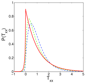
For $\epsilon\neq 1$ this integral may be calculated numerically. However for $\epsilon=1$ it might be evaluated analytically. In particular, for $T_{xx}>0$ we obtain

$$P(T_{xx})=\frac{2}{\sqrt{6}}\frac{e^{-(\sqrt{24}-4)T_{xx}}}{(5-\sqrt{24})}-8e^{-T_{xx}},$$ (25)

and for $T_{xx}<0$

$$P(T_{xx})=\frac{2}{\sqrt{6}}\frac{e^{(\sqrt{24}+4)T_{xx}}}{(5+\sqrt{24})}.$$ (26)

The distribution (26) is shown in Fig. 1 together with results for different $\epsilon$-values obtained by numerical evaluation of the integral (24). Note that the distributions are here given in terms of $\langle T_{xx}\rangle=1+\epsilon^{2}$.

Figure 1: (color online) The distribution $P(T_{xx})$ for $\epsilon=1$ (dash-dotted line), $\epsilon=0.5$ (dashed line), and $\epsilon=0$ (solid line). The stress tensor component $T_{xx}$ is measured in terms of the mean value $\langle T_{xx}\rangle$.

To repeat the calculations for the component $T_{xy}$ we need the following correlators

$$\langle uu_{xy}\rangle=0,~{}\langle u_{x}u_{xy}\rangle=0,\langle u_{y}u_{xy}\rangle=0,\langle u_{xy}^{2}\rangle=\frac{1}{8}$$ (27)

for the 2D case. The correlation matrix turns out to be diagonal. Then the characteristic function

$$\theta(a) = 2[(2+(a/2)^{2})(2+(\epsilon a/2)^{2})(1+(a/2)^{2})$$ (28)

$$(1+(\epsilon a/2)^{2})]^{-1/2}$$

defines the distribution $P(T_{xy})$. For $\epsilon=1$ the integral (24) may, as above, be performed analytically to give

$$P(T_{xy})=2e^{-2|T_{xy}|}-\sqrt{2}e^{-2\sqrt{2}|T_{xy}|}.$$ (29)

Figure 2: (color online) The distribution $P(T_{xy})$ for $\epsilon=1$ (dash-dotted line) and $\epsilon=0$ (solid line). The stress tensor component $T_{xy}$ is measured in terms of mean value $\sqrt{\langle T_{xy}^{2}\rangle}$.

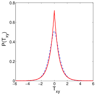
The distributions $P(T_{xy})$ in (29) are shown in Fig. 2 for the two cases $\epsilon=0$ and $\epsilon=1$. Only two cases are shown because of the small differences in $P(T_{xy})$ for different $\epsilon$-values. The distributions are in this case given in terms of $\sqrt{\langle T_{xy}^{2}\rangle}$, where $\langle T_{xy}^{2}\rangle=\frac{3}{8}(1+\epsilon^{4})$.

Three-dimensional case. In this case the expressions in (III) are to be replaced by

$$\langle uu_{xx}\rangle=-\frac{1}{3},\,\,\langle u_{x}^{2}\rangle=\frac{1}{3},\,\,$$ (30)

$$\langle uu_{x}\rangle=0,\,\,\langle u_{x}u_{xx}\rangle=0,\,\,\langle u_{xx}^{2}\rangle=\frac{1}{5}$$

and (27) by

$$\langle uu_{xy}\rangle=0,~{}\langle u_{x}u_{xy}\rangle=0,\langle u_{y}u_{xy}\rangle=0,\langle u_{xy}^{2}\rangle=\frac{1}{15}.$$ (31)

Accordingly the correlation matrix (19) is

$$K_{u}=\left(\matrix{1&-1/3\cr-1/3&1/5\cr}\right),\,\,K_{u}^{-1}=\frac{1}{4}\left(\matrix{9&15\cr 15&45\cr}\right).$$ (32)

The joint probability function of two RGFs $u$ and $u_{xx}$ then takes the following form

$$f(u,u_{xx})=\frac{\sqrt{45}}{2\pi}\exp\left\{-\frac{9u^{2}+30uu_{xx}+45u_{xx}^{2}}{8}\right\}.$$ (33)

The characteristic function defining the distribution $P(T_{xx})$ is

$$\theta(a)=\frac{45}{(3/2-ia)(ia+15/4+9\sqrt{5}/4)}$$

$$\frac{1}{(ia+15/4-9\sqrt{5}/4)}$$ (34)

and, correspondingly,

$$P(T_{xx})=\frac{5}{(7\sqrt{5}-15)}e^{-\frac{9\sqrt{5}-15}{4}T_{xx}}-\frac{15}{2}e^{-\frac{3}{2}T_{xx}}$$ (35)

for $T_{xx}>0$, and

$$P(T_{xx})=\frac{5}{(7\sqrt{5}+15)}e^{\frac{9\sqrt{5}+15}{4}T_{xx}}$$ (36)

for $T_{xx}<0$. Identical expressions hold for the two other diagonal components.

In a similar way we obtain the distribution function for the off-diagonal components $\alpha\neq\beta$. For the specific case $\epsilon=1$ we have according to Eq. (31)

$$\theta(a)=\frac{2}{[3+(a/2)^{2}][1+(a/2)^{2}]},$$ (37)

and

$$P(T_{xy})=\frac{15}{4}e^{-3|T_{xy}|}-\frac{3\sqrt{15}}{4}e^{-\sqrt{15}|T_{xy}|}.$$ (38)

The expression for the other off-diagonal components are, of course, identical.

IV Distribution of quantum potential

The quantum or internal force in Eq. (11) in the hydrodynamic formulation is defined by the quantum potential $V_{QM}$. In terms of the RGFs $u,~{}v$ it may be written as

$$V_{QM}=-V_{x}-V_{y},$$ (39)

$$V_{x}=\frac{uu_{xx}+vv_{xx}+u_{x}^{2}+v_{x}^{2}}{u^{2}+v^{2}}-\left(\frac{uu_{x}+vv_{x}}{u^{2}+v^{2}}\right)^{2},$$

$$V_{y}=\frac{uu_{yy}+vv_{yy}+u_{y}^{2}+v_{y}^{2}}{u^{2}+v^{2}}-\left(\frac{uu_{y}+vv_{y}}{u^{2}+v^{2}}\right)^{2}.$$

The second derivatives might be eliminated using the Schrödinger equations for $u$ and $v$, i. e., $u_{xx}+u_{yy}=-u,~{}~{}v_{xx}+v_{yy}=-v$. As a result we have

$$V_{QM}=1-\frac{(uv_{x}-vu_{x})^{2}+(uv_{y}-vu_{y})^{2}}{{\rho}^{2}}.$$ (40)

which implies

$$-\infty\leq V_{QM}\leq 1.$$ (41)

The distribution of the quantum potential is given by

$$P(V_{QM})=\frac{1}{2\pi}\int\exp(-iaV_{QM})\theta(a)da,$$ (42)

where

$$\theta(a)=\langle\exp(iaV_{QM})\rangle=\int d^{6}\overrightarrow{X}f(\overrightarrow{X})\exp(iaV_{QM}),$$ (43)

$f(\overrightarrow{X})$ is given by the same formula as (18), however, with vector $\overrightarrow{X}^{+}=(u,v,u_{x},v_{x},u_{y},v_{y})$ with the same correlators as (19).

For (43) we may now write with $\epsilon=1$, which is the only case accessible in closed analytic form,

$$\theta(a)=\frac{1}{2\pi}\int dudv\Gamma_{x}\Gamma_{y}\exp\left[-\frac{1}{2}(u^{2}+v^{2})+ia\right],$$ (44)

with

$$\Gamma_{x}=\frac{1}{\pi}\int du_{x}dv_{x}\exp\left\{-u_{x}^{2}-v_{x}^{2}+\frac{ia(uu_{x}-vv_{x})^{2}}{\rho^{2}}\right\}.$$ (45)

The same expression holds for $\Gamma_{y}$. The integration in (45) gives

$$\Gamma_{x}\Gamma_{y}=\frac{-i\rho}{a-i\rho}.$$ (46)

Substituting (46) into (44) we obtain

$$\theta(a)=-i\int_{0}^{\infty}\frac{drr^{3}}{a-ir^{2}}\exp(ia-r^{2}/2)$$ (47)

where $r=\sqrt{\rho}$. Finally, substituting that into (42) we obtain the distribution function for the quantum potential

$$P(V_{QM})=\frac{1}{2(3/2-V_{QM})^{2}}.$$ (48)

Figure 3: (color online) The distribution of the quantum potential (48) for $\epsilon=1$ compared to numerical histogram based on the Berry function in Eq. (49).

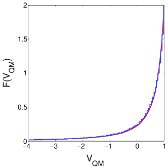
The distribution (48) is normalized as $\int_{-\infty}^{1}P(V)dV=1$. The distribution of $P(V_{QM})$ is shown in Fig. 3 and compared to a numerical computation of the same statistics based on the Berry conjecture for chaotic wave functions [Berry, 1977]

$$\psi(r)=\frac{1}{\sqrt{A}}\sum_{n}a_{n}e^{i{\bf k}_{n}{\bf\cdot r}}.$$ (49)

Here $A$ is the area of the random monochromatic plane wave field with $|{\bf k}_{n}|^{2}=1$ and the amplitudes for the random plane waves obey the relation $\langle a_{n}^{2}\rangle=\frac{1}{N}$. The Berry function in Eq. (49) corresponds to $\epsilon=1$.

V Numerical simulations of scattering states in an open chaotic electron billiard

A billiard becomes an open one when it is connected to external reservoirs, for example, via attached leads. A stationary current through the system may be induced by applying suitable voltages to the reservoirs (or by a microwave power source as in Section VI). Here we consider hard-walled Sinai-type billiards with two opposite normal leads. A first step towards a numerical simulations of the quantum stress tensor is to find the corresponding scattering states by solving the Schrödinger equation $-\nabla^{2}\psi=k^{2}\psi$ for the entire system. The numerical procedure for this is well known. Thus we use the finite difference method for the interior of the billiard in combination with the Ando boundary condition [Berggren et al., 2002; Ando, 1991] for incoming, reflected and transmitted solutions in the straight leads. Once a scattering wave function has been computed in this way the fraction residing in the cavity itself is extracted for the statistical analysis. To ensure statistical independence of the real and imaginary parts $u$ and $v$ a global phase is removed as discussed in Ref. [Saichev et al., 2002]. By this step we also find the value of $\epsilon$. The interior wave function is then normalized as defined in Section III.

For the numerical work it is convenient to make the substitution $x\rightarrow x/d$ and $y\rightarrow y/d$ where $d$ is the width of the leads. Here we use dimensionless energy $k^{2}=E/E_{0},E_{0}=\hbar^{2}/(2md^{2}$). (In the case of a semiconductor billiard referred to in the introduction, the mass $m$ should be the effective conduction band mass $m^{*}$). Below we consider the specific case of small wave lengths $\lambda$ as shown in Fig. 4. We will also comment on the case when $\lambda$ is large compared to the dimensions of the cavity.

Figure 4: View of the scattering wave function in the open Sinai billiard for the case (A) shown in Fig. 5 for $k^{2}=30.878$ in dimensionless units (see text) and for small aspect ratio $d/L$ = 2/67 (ratio between the widths of the leads and the billiard). The system is asymmetric because the two opposite leads are slightly off the middle symmetry line of the nominal billiard. Only the lowest channel is open in the leads.

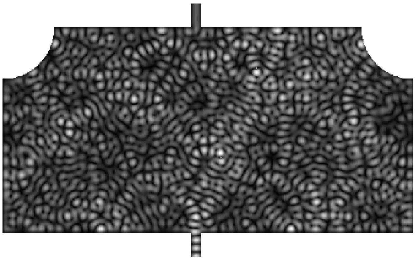
To ensure that the scattering wave function complies with a complex RGF we consider a small aspect ratio $d/L$ as in Fig. 4 (see also Ref. [Berggren et al., 2002]). The actual numerical size of the Sinai billiard in Fig. 4 is chosen as: height 346 (along transport), width ($L$) 670, radius 87, and 20 for the number of grid points across the wave guides ($d$). Within this configuration we now only excite scattering wave function with characteristic wave lengths $\lambda\ll L$. As expected from Fig. 4 the wave function statistics show that both real and imaginary parts, $u$ and $v$, obey Gaussian statistics to a high degree of accuracy. Results for transmission $T$ and $\epsilon$ are are shown in Fig. 5.

Figure 5: (color online) The transmission probability $T$ (solid line) and $\epsilon$ (dashed line) as function of the dimensionless energy $k^{2}$ for the Sinai billiard in Fig. 4. Two open circles labeled show the case with maximal $\epsilon=0.75$ (A) and with the minimal $\epsilon=0$ (B). At most only one channel is open in the leads.

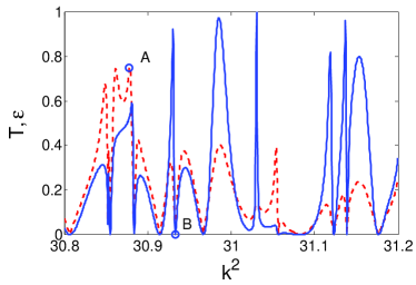
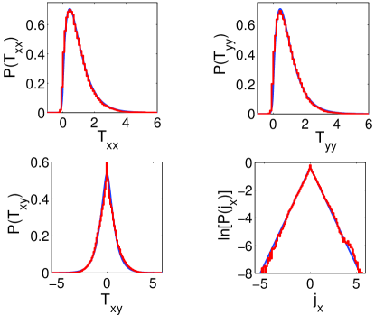
The corresponding distributions for the QST components are given in Figs. 6 and 7 supplemented by the distributions for $j_{x}$ with the $x$ axis directed along transport. There is indeed an overall good agreement between theory and simulations. However, in the statistics for $j_{x}$ in Fig. 6 one notices a tiny difference at small values of $j_{x}$. The reason is that there is a net current at this value of $\epsilon$, which is not incorporated in our choice of analytic isotropic RGFs. The deviation is, however, much too small to have an impact on the statistical analysis presented here because the net current is such a tiny fraction of the entire current pattern within the cavity. The case B with $\epsilon=0$ implies that the scattering wave function in the cavity is real (standing wave with transmission $T=0$ as seen from Fig. 5). Therefore there is no current within the cavity.

Figure 6: (color online) Analytic and numerically simulated distributions of the components of the QST and probability density current $j_{x}$ along the transport axis for the case A shown in Fig. 5 ($\epsilon=0.75$). As in Figs. 1 and 2 the diagonal components are measured in terms of their mean values while $T_{xy}$ and $j_{x}$ are given in terms of $\sqrt{\langle T_{xy}^{2}\rangle}$ and $\sqrt{\langle j_{x}^{2}\rangle}$, respectively. Solid lines refer to analytic results for RGFs (Section III and Ref. [Saichev et al., 2002]) and histograms to the present numerical modeling. Because of the close agreement between the two cases differences are barely resolved.

Figure 7: (color online) Analytic and numerically simulated distributions of the components of the QST for the case B in Fig. 5 ($\epsilon=0$). The simulated distribution for $T_{yy}$ is nearly identical to $P(T_{xx})$ and therefore not shown here. Because $\epsilon$ vanishes there is not any current within the cavity. (The choice of lines in the graphs and units are the same as in Fig. 6. Because the close agreement between theory and simulations differences are hardly noticeable.)

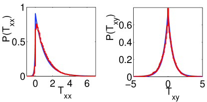
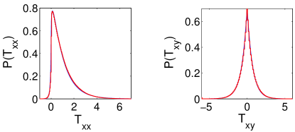
The agreement with the analytic results for RGFs and the present numerical modeling for billiards of finite size is obviously good in the range of energies explored here. In order to smooth fluctuations in the distributions of the stress tensor we have averaged over the energy window shown in Fig. 5 (without scaling $\epsilon$ to 1 in contrast to Fig. 11 of Section VI). In this way one finds a perfect agreement between theory and numerical simulations as shown in Fig. 8. For future reference we note that the presence of net currents through the billiard appears to have little or no influence on the distributions for the present two-lead configuration and choice of energy range. We also note that the present results are not sensitive to the position of the leads. For example, we have also performed simulations for Sinai billiards with one dent only and with the leads attached at corners.

Figure 8: (color online) Analytic and numerically simulated distributions of the components of stress tensor $T_{xx}$ and $T_{xy}$ averaged over the energy window given in Fig. 5. The theoretical curves are obtained also by averaging over computed $\epsilon$-values shown in Fig. 5. (The choice of lines and units are the same as in Fig. 6. The agreement between theory and simulations is, however, excellent, hence any small differences are not resolved on the scale shown here.)

We now turn to the complementary case of long wave lengths (low energies). The low energy regime is achieved for large aspect ratio $d/L$ which selects wave functions with $\lambda$ a few times less than $L$. Moreover a low energy incoming wave often excites bouncing modes. Numerics for the case $k^{2}=12$ and large aspect ratio $d/L=1/7$ show that the scattering wave function may be rather different from a complex RGF. Hence the corresponding distributions for individual states deviate appreciably from the theoretical RGF predictions in Section III. However, by averaging over a wide energy window, as above, one closes in on theory. In this way one introduces an ensemble that, for practical purposes, mimics the random Gaussian case. This aspect may be useful in experimental circumstances in which the short wave length limit might be hard to achieve.

VI Experimental studies

Figure 9: (color online) Sketch of the microwave billiard. The basic size of the billiard is $16\,\mathrm{cm}\times 21\,\mathrm{cm}$. The attached leads have a width of 3 cm. The central shaded field ($10\,\mathrm{cm}\times 14\,\mathrm{cm}$) indicates the region where the data have been collected. The measurement grid size was 2.5 mm. The gray regions at the end of the two leads indicate absorbers to mimic infinitely long channels. The crosses indicate the antennas in the system and the winding path illustrates how the third probing antenna is moved across the billiard during measurements.

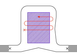
In quasi-2D resonators there is, as outlined in the introduction, a one-to-one correspondence between the TM modes of the electromagnetic field and the wave functions of the corresponding quantum billiard [Stöckmann, 1999]. The $z$-component of the electromagnetic field $E_{z}$ corresponds to the quantum-mechanical wave function $\psi$, and the wave number $k^{2}=\omega^{2}/c^{2}$ to the quantum-mechanical eigenenergy, where $\omega$ is the angular frequency of the TM mode and $c$ the speed of light. In the present study a rectangular cavity ($16\,\mathrm{cm}\times 21\,\mathrm{cm}$) with rounded corners has been used, with two attached leads with a width of 3 cm. Antennas placed in the leads acted as source and drain for the microwaves (see Fig. 9). Two wedge-shaped obstacles had been attached to two sides of the billiard to avoid any bouncing ball structures in the measurement. The same system has been used already for the study of a number of transport studies [Barth and Stöckmann, 2002; Kim et al., 2003] and for the statistics of nodal domains and vortex distributions [Kuhl, 2007]. A more detailed description of the experimental setup can be found in Ref. [Kuhl et al., 2000]. The field distribution inside the cavity has been obtained via a probe antenna moved on a grid with a step size of 2.5 mm. To avoid boundary effects, only data from the shaded region (see Fig. 9) has been considered in the analysis.

Figure 10: The figure shows different quantities obtained from the measurement at the frequency $\nu=8.5\,\mathrm{GHz}$. In (a) the intensity of the wave function is shown and in (b) its phase. The plot (c) shows the Poynting vector of the system being equivalent to the probability current density in quantum mechanics. In (d)-(f) different components of the QST are shown, namely $xy$ (d), $xx$ (e) and $yy$ component (f). Dark areas indicate higher values.

The transmission from the source to the probe antenna has been measured on the frequency range from 5.5 to 10 GHz with a step size of 20 MHz, corresponding to wave lengths from 3 to 5 cm. The transmission is proportional to the electric field strength, i. e. to the wave function, at the position of the probe antenna. This assumes that the leak current into the probe antenna may be neglected.

To check this we compared the experimentally obtained distribution of wave function intensities $\rho=\left|\psi\right|^{2}$ with the modified Porter-Thomas distribution (see e. g. Ref. [Saichev et al., 2002])

$$p\left(\left|\psi\right|^{2}\right)=\mu\exp\left(-\mu^{2}\left|\psi\right|^{2}\right)\,I_{0}\left(\mu\sqrt{\mu^{2}-1}\left|\psi\right|^{2}\right)$$ (50)

where

$$\mu=\frac{1}{2}\left(\epsilon+\frac{1}{\epsilon}\right)\qquad\textnormal{and}\qquad\epsilon^{2}=\langle v^{2}\rangle/\langle u^{2}\rangle$$ (51)

Here $\epsilon$ has not been fitted, but was taken directly from the experimentally obtained values for $\langle u^{2}\rangle$ and $\langle v^{2}\rangle$, where we have ensured that $\langle uv\rangle=0$ by applying a proper phase rotation as in [Saichev et al., 2002] and commented on in Section V). Whenever $\chi^{2}$, the weighted squared difference of the experimental data and the modified Porter-Thomas distribution, was below $\chi_{\mathrm{cutoff}}$=1.1, the pattern has been selected for the final analysis of the statistics for the QST components.

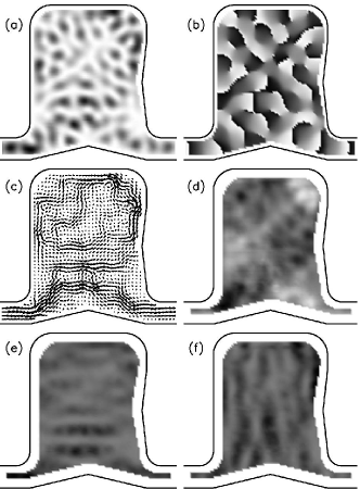
Since the wave functions are experimentally known, including their phases, the quantum-mechanical probability density ${\bf j}=\mathrm{Im}\psi^{*}{\bf\nabla}\psi$, and the components of the QST can be obtained from the measurement. As mentioned, distributions of current densities and related quantities have already been discussed previously in a number of papers (see e. g. Ref. [Barth and Stöckmann, 2002; Kim et al., 2003]), but the QST has not been studied experimentally before. As an example Fig. 10 show intensity (a) and the phase (b) of the measured field at one frequency, as well as the probability current (c) and different components of the stress tensor (d - f).

The analysis of the data has been performed in dimensionless coordinates ${\bf x}=k{\bf r}$. Since $u$ and $v$ are two independent random wave fields we may rescale the imaginary part to obtain $\epsilon$ values of one, thus mapping the experimental result to the situation of a completely open billiard. This step made it easy to superimpose the results from many field patterns of different frequencies which originally had different $\epsilon$ values. For the analysis all wave functions passing the $\chi^{2}$ test mentioned above have been used. Altogether 83 of 225 possible patterns have been taken in the analysis.

Figure 11: (color online) Results for the experimental statistical distributions for the components of the QST stress tensor obtained by a superposition of all experimental data scaled to $\epsilon=1$ as explained in the text. The solid lines correspond to the theoretical predictions in Section III for $\epsilon=1$.

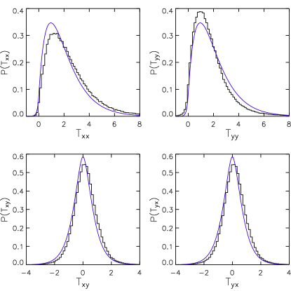
Figure 11 shows the distribution of the QST components obtained in this way. In addition the theoretical curves are shown as solid lines. From the figure we see that there is a good overall agreement between experiment and theory, but also that non-statistical deviations are unmistakable.

Deviations between experiment and theory had already been found by us in the past in an open microwave billiard, similar to the one used in the present experiment, in the distribution of current components [Barth and Stöckmann, 2002; Kim et al., 2003]. For the vertical $y$ component a complete agreement between experiment and theory was found, but for the horizontal $x$ component the experimental distribution showed, in contrast to theory, a pronounced skewness. The origin of this discrepancy was a net current from the left to the right due to source and drain in the attached wave guides. In a billiard with broken time-reversal symmetry without open channels, a complete agreement between experiment and theory had been found, corroborating the net current hypothesis.

Figure 12: Plot of the net current as it is defined in Eq. (52). The shaded regions are indicating three different regimes of net current strength which had been used in the later analysis.

For a quantitative discussion of the net current we introduced the normalized net current for each pattern

$$\mathbf{j}_{\mathrm{net}}=\frac{\langle\mathbf{j}\rangle}{\langle|\mathbf{j}|\rangle}.$$ (52)

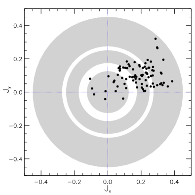
where the average is over all positions in the shaded region in Fig. 9. In Fig. 12 the $y$ component of $\mathbf{j}_{\mathrm{net}}$ is plotted versus its $x$ component for each wave function. One notices an average net current pointing from left to right, with an angle of about twenty degrees in an upward direction. For the analysis we discriminated between three regimes for the strength of the net current. Additionally we performed a coordinate transformation such that for each pattern the vector of the net current is aligned along the positive $x$-axis. This rotation has been done for all experimental and numerical results in this section.

Figure 13: (color online) Histograms of the QST distributions obtained from experimental data. The thick lines corresponds to the smallest net currents (see Fig. 12), the thin lines to intermediate ones and the dashed lines to ones with the largest net current. As in Fig. 11 the solid lines correspond to the theoretical predictions in Section III for $\epsilon=1$.

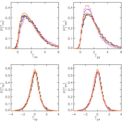
In Fig. 13 the results for the three different regimes of net current strengths are shown. For the distributions of the $xx$ and the $yy$ component of the QST, a clear dependence on the net current strength is found, where the deviations from theory increase with an increasing net current. $T_{xy}$ is only slightly affected by the net current, if at all. In the limit of a tiny net current, all experimental distributions approach the theoretical ones.

Figure 14: (color online) Histograms of the QST components obtained from the simulations according to the wave function in Eq. (53). As in previous figure, the thick lines correspond to low, thin to intermediate and dashed lines to large net currents.

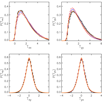
To further test the influence of the net current on the distributions of the stress tensor, we performed a numerical simulation with random plane waves. Each random wave field was calculated on an area of $500\,\mathrm{mm}\times 500\,\mathrm{mm}$, with a grid size of 2.5 mm. The random wave field consisted of 500 plane waves with random directions and amplitudes. The frequency used for the numerics was $\nu=5\,\mathrm{GHz}$. To introduce the net current we first performed a random superposition of plane waves according to Eq. (49), and then added a normalized plane wave with the wave vector $K^{\prime}$ pointing in the same direction as the net current observed in the experiment,

$$\psi(r)=\frac{1}{\sqrt{A}}\left(a^{\prime}e^{i{\bf K^{\prime}\cdot r}}+\sum_{n=1}^{N}a_{n}e^{i{\bf k}_{n}{\bf\cdot r}}\right)$$ (53)

The strength of the resulting net current was adjusted by a prefactor $a^{\prime}$. The best agreement between the experiment and the numerics was found for $a^{\prime}=0.45$. To get sufficient statistics we averaged over 200 different wave functions. Thus a pattern similar to the one shown in Fig. 12 was obtained with a cloud of dots extending over all three regimes of net current considered with its center in the central regime.

Fig. 14 shows the distributions for the QST components for numerical data derived from Eq. (53). The same three regimes as for the experimental study have been used. The results from this type of simulation are in good qualitative agreement with the experimental results. In particular the deviations from the theory in Section III increase monotonously with the net current, just as in the experiment.

An obvious question is why these net current effects are unimportant in the simulations for the Sinai billiard presented in Section V. One may argue that the number of independent plane waves entering at a given frequency is given by the circumference of the billiard divided by $\lambda/2$, where $\lambda$ is the wavelength. Also the width of each wave guide is of the order of $\lambda/2$, i. e. the relative net current is approximately given by the total widths of all openings divided by the circumference of the billiard. Following this argumentation the net current in the experiments amounted to about 10 percent of the total current, whereas in the simulations for the Sinai billiard it was smaller by a factor of 10; i.e. too small to be of any importance in the simulations.

We have shown that in the limit of small net currents, the distributions of QST components obtained from the experiment are well described by means of the random plane wave model and the analytic distributions in Section III. On the other hand net currents are unavoidable in open systems. As indicated by the simulations for a Sinai billiard in Section V, the magnitudes and effect on the different stress tensor distributions may be sensitive to geometry and energy. Hence it remains an open task for theory to incorporate net currents in order to allow a more realistic comparison with present experimental results.

VII Acknowledgements

The theoretical part of this joint project has been carried out by the two theory groups at Linköping University and Kirensky Institute of Physics. Measurements and the data interpretation have been performed by the quantum chaos group at the Philipps-Universität Marburg.

K.-F. B., D. M. and A.F. S. are grateful to the Royal Swedish Academy of Sciences for financial support for the theory part of this work (“Academy Programme for Collaboration between Sweden and Russia”). R. H., U. K. and H.-J. S. thank the Deutsche Forschungsgemeinschaft for financial support of the experiments (via Forschergruppe 760 “Scattering systems with complex dynamics”). Finally, KFB is grateful to Andrew W. Rappe, Jianmin Tao and Irina I. Yakimenko for informative discussions on the concept of quantum stress.

References

- Stöckmann (1999) H.-J. Stöckmann, Quantum Chaos - An Introduction (University Press, Cambridge, 1999).
- Guhr et al. (1998) T. Guhr, A. Müller-Groeling, and H. A. Weidenmüller, Phys. Rep. 299, 189 (1998).
- Berggren and Åberg (2001) K.-F. Berggren and S. Åberg, eds., Quantum Chaos Y2K - Nobel Symposium 116 (Physica Scripta, Stockholm, 2001).
- Fyodorov et al. (2005) Y. V. Fyodorov, T. Kottos, and H.-J. Stöckmann, eds., Special Issue: Trends in Quantum Chaotic Scattering, Journal of Physics A: Mathematical and General (Institute of Physics, Bristol, 2005).
- Davies (1998) J. H. Davies, The Physics of Low-dimensional Semiconductors: An Introduction (Cambridge University Press, Cambridge, 1998).
- Saichev et al. (2002) A. I. Saichev, H. Ishio, A. F. Sadreev, and K.-F. Berggren, J. Phys. A 35, L87 (2002).
- Kim et al. (2005) Y.-H. Kim, U. Kuhl, H.-J. Stöckmann, and P. W. Brouwer, Phys. Rev. Lett. 94, 036804 (2005).
- Berry and Dennis (2000) M. V. Berry and M. R. Dennis, Proc. R. Soc. Lond. A 456, 2059 (2000).
- Saichev et al. (2001) A. I. Saichev, K.-F. Berggren, and A. F. Sadreev, Phys. Rev. E 64, 036222 (2001).
- Berggren et al. (2002) K.-F. Berggren, A. F. Sadreev, and A. A. Starikov, Phys. Rev. E 66, 016218 (2002).
- Dennis (2007) M. R. Dennis, Eur. Phys. J. Special Topics 145, 191 (2007).
- Sadreev and Berggren (2004) A. F. Sadreev and K.-F. Berggren, Phys. Rev. E 70, 026201 (2004).
- Barth and Stöckmann (2002) M. Barth and H.-J. Stöckmann, Phys. Rev. E 65, 066208 (2002).
- Kim et al. (2003) Y.-H. Kim, M. Barth, U. Kuhl, and H.-J. Stöckmann, Prog. Theor. Phys. Suppl. 150, 105 (2003).
- Pauli (1933) W. Pauli, Quantentheorie, Handbuch der Physik XXIV (Springer, Berlin, 1933).
- Pauli (1980) W. Pauli, General Principles of wave mechanics, Handbuch der Physik XXIV (Springer, Berlin, 1980).
- Misner et al. (1973) C. W. Misner, K. S. Thorne, and J. A. Wheeler, Gravitation (W. H. Freeman, New York, 1973).
- Nielsen and Martin (1985) O. H. Nielsen and R. M. Martin, Phys. Rev. B 32, 3780 (1985).
- Folland (1986) N. O. Folland, Phys. Rev. B 34, 8296 (1986).
- Godfrey (1988) M. J. Godfrey, Phys. Rev. B 37, 10176 (1988).
- Shenoy (2004) V. B. Shenoy, in The Handbook of Nanotechnology: Nanometer Structures, Theory, Modeling and Simulations, edited by A. Lakhtakia (SPIE press, 2004), pp. 256–316.
- Höntschel et al. (2004) J. Höntschel, R. Stenzel, and W. Klix, IEEE Trans. on Electron Devices 51, 684 (2004).
- Godfrey (1990) M. J. Godfrey, J. Phys. B 23, 2427 (1990).
- Tao et al. (2008) J. Tao, G. Vignale, and I. V. Tokatly, Phys. Rev. Lett. (in press 2008).
- Rogers and Rappe (2002) C. L. Rogers and A. M. Rappe, Phys. Rev. B 65, 224117 (2002).
- Maranganti et al. (2002) R. Maranganti, P. Sharma, and L. Wheeler, J. Aerosp. Eng. 20, 22 (2002).
- Crook et al. (2003) R. Crook, C. G. Smith, A. C. Graham, I. Farrer, H. E. Beere, and D. A. Ritchie, Phys. Rev. Lett. 91, 246803 (2003).
- Sridhar (1991) S. Sridhar, Phys. Rev. Lett. 67, 785 (1991).
- Stein and Stöckmann (1992) J. Stein and H.-J. Stöckmann, Phys. Rev. Lett. 68, 2867 (1992).
- Gokirmak et al. (1998) A. Gokirmak, D.-H. Wu, J. S. A. Bridgewater, and S. M. Anlage, Rev. Sci. Instrum. 69, 3410 (1998).
- Lauber et al. (1994) H.-M. Lauber, P. Weidenhammer, and D. Dubbers, Phys. Rev. Lett. 72, 1004 (1994).
- Dembowski et al. (1999) C. Dembowski, H.-D. Gräf, R. Hofferbert, H. Rehfeld, A. Richter, and T. Weiland, Phys. Rev. E 60, 3942 (1999).
- Laurent et al. (2007) D. Laurent, O. Legrand, P. Sebbah, C. Vanneste, and F. Mortessagne, Phys. Rev. Lett. 99, 253902 (2007).
- Berry (1977) M. V. Berry, J. Phys. A 10, 2083 (1977).
- Madelung (1927) E. Madelung, Z. Phys. 40, 322 (1927).
- Bialynicki-Birula et al. (1992) I. Bialynicki-Birula, M. Cieplak, and J. Kaminski, The Theory of Quanta (Oxford University Press, Oxford, 1992).
- Holland (1993) P. R. Holland, The quantum theory of motion : an account of the de Broglie-Bohm causal interpretation of quantum mechanics (Cambridge Univ. Pr., Cambridge, 1993).
- Wyatt (2005) R. E. Wyatt, Quantum Dynamics with Trajectories, Introduction to Quantum Hydrodynamics, vol. 28 of Interdisciplinary Applied Mathematics (Springer, New York, 2005).
- McDonald and Kaufman (1988) S. W. McDonald and A. N. Kaufman, Phys. Rev. A 37, 3067 (1988).
- Ebeling (1984) K. J. Ebeling, in Semi-Classical Approximation in Quantum Mechanics. In: Mathematical Physics and Applied Mathematics 7, Contemporary Mathematics 5. Dordrecht etc., edited by W. P. Mason and R. N. Thurston (Academic Press, New York, 1984), vol. 17, p. 233.
- Ando (1991) T. Ando, Phys. Rev. B 44, 8017 (1991).
- Kuhl (2007) U. Kuhl, Eur. Phys. J. Special Topics 145, 103 (2007).
- Kuhl et al. (2000) U. Kuhl, E. Persson, M. Barth, and H.-J. Stöckmann, Eur. Phys. J. B 17, 253 (2000).