The stable magnetic field of the fully-convective star V374 Peg

Abstract

We report in this paper phase-resolved spectropolarimetric observations of the rapidly-rotating fully-convective M4 dwarf V374 Peg, on which a strong, mainly axisymmetric, large-scale poloidal magnetic field was recently detected. In addition to the original data set secured in 2005 August, we present here new data collected in 2005 September and 2006 August.

From the rotational modulation of unpolarised line profiles, we conclude that starspots are present at the surface of the star, but their contrast and fractional coverage are much lower than those of non-fully convective active stars with similar rotation rate. Applying tomographic imaging on each set of circularly polarised profiles separately, we find that the large-scale magnetic topology is remarkably stable on a timescale of 1 yr; repeating the analysis on the complete data set suggests that the magnetic configuration is sheared by very weak differential rotation (about 1/10th of the solar surface shear) and only slightly distorted by intrinsic variability.

This result is at odds with various theoretical predictions, suggesting that dynamo fields of fully-convective stars should be mostly non-axisymmetric unless they succeed at triggering significant differential rotation.

1 Introduction

Most cool stars exhibit demonstrations of activity such as cool surface spots, coronal activity or flares, usually attributed to magnetic fields. The current understanding is that these magnetic fields are generated at the surfaces and in the convective envelopes of cool stars through dynamo processes, involving cyclonic motions of plasma and rotational shearing of internal layers. In partly-convective Sun-like stars, dynamo processes are thought to concentrate where rotation gradients are supposedly largest, i.e., at the interface layer between their radiative cores and convective envelopes. Cool stars with masses lower than 0.35 ${\rm M}_{\odot}$ being fully convective (Chabrier & Baraffe, 1997), they lack the thin interface layer presumably hosting solar-type dynamo processes and are thought to rotate mainly as rigid bodies (Barnes et al., 2005; Küker & Rüdiger, 2005); yet they are both very active (e.g., Delfosse et al., 1998) and strongly magnetic (Saar & Linsky, 1985; Johns-Krull & Valenti, 1996; Reiners & Basri, 2007).

This led theoreticians to propose that the intense activity and strong magnetism of fully convective dwarfs may be due to non-solar dynamo processes, in which cyclonic convection and turbulence play the main roles while differential rotation contributes very little (e.g., Durney et al., 1993); the exact mechanism capable of producing such fields is however still a debated issue. The most recent numerical dynamo simulations suggest that these stars are actually capable of producing large-scale magnetic fields, although they disagree on the actual properties of the large scale field. While some find that fully-convective stars rotate as solid bodies and host purely non-axisymmetric large-scale fields (Küker & Rüdiger, 2005; Chabrier & Küker, 2006), others diagnose that these stars should succeed at triggerring differential rotation and thus produce a net axisymmetric poloidal field (e.g., Dobler et al., 2006).

Existing observational data on fully convective dwarfs do not completely agree with any of these models. Observations of low-mass stars indicate that surface differential rotation vanishes with increasing convective depth, so that fully-convective stars rotate mostly as solid bodies (Barnes et al., 2005). At first sight, this result confirms nicely the predictions of Küker & Rüdiger (2005), leading one to expect fully-convective stars to host purely non-axisymmetric large-scale fields (Chabrier & Küker, 2006). However, spectropolarimetric data of the rapidly rotating M4 dwarf V374 Peg (G 188-38, GJ 4247, HIP 108706) collected with ESPaDOnS for almost three complete rotation periods over nine rotation cycles (Donati et al., 2006, hereafter D06) demonstrated that this fully-convective star hosts a strong mostly-axisymmetric poloidal field despite rotating almost rigidly, in contradiction with theoretical expectations.

In this new paper, we present and analyse spectropolarimetric data of V374 Peg collected with ESPaDOnS at three different epochs, 2005 August (i.e., those used in D06), 2005 September (providing only partial coverage of the rotation cycle) and 2006 August (providing full, though not very dense, coverage of the rotation cycle). First, we briefly describe the new observations and the Zeeman detections we obtained. We then apply tomographic imaging to our data sets and characterise the spot distributions and magnetic topologies at the surface of V374 Peg in both 2005 and 2006; from the observed temporal evolution of the magnetic topology, we also estimate both the differential rotation and the long-term magnetic stability of V374 Peg. Finally, we discuss the implications of our results for our understanding of the dynamo processes operating in fully-convective stars.

Table 1: Journal of observations. Subsets of observations collected sequentially on the same night (with no time gaps) are listed on a single line. Columns 1–7 list the UT date, the number of observations in each subset, the heliocentric Julian date, the UT time, the exposure time, the peak signal to noise ratio (per 2.6 km s^-1 velocity bin) and the rms noise level (relative to the unpolarised continuum level and per 1.8 km s^-1 velocity bin) in the average circular polarization profile produced by Least-Squares Deconvolution (see text). The rotational cycle $E$ from the ephemeris of equation (1) is given in column 8. Whenever several observations are present in a subset, cols. 3, 4 and 8 list the values corresponding to the first and last subset observations, whereas cols. 6 and 7 mention the minimum and maximum values reached within the subset.

Date	$n_{\rm obs}$	HJD	UT	$t_{\rm exp}$	S/N	$\sigma_{\rm LSD}$	Cycle
		(2,453,000+)	(h:m:s)	(s)		($10^{-4}I_{\rm c}$)
2005
Aug 19	6	601.78613–601.87607	06:43:29–08:52:59	4 $\times$ 300.0	145–170	6.0–7.7	0.00–0.20
Aug 19	12	601.94413–602.13790	10:30:60–15:10:01	4 $\times$ 300.0	99–172	5.6–11.3	0.35–0.79
Aug 21	23	603.75042–604.19199	05:52:00–15:15:52	4 $\times$ 300.0	137–208	5.7–7.8	4.41–5.40
Aug 23	23	605.73892–606.13069	05:35:25–14:59:33	4 $\times$ 300.0	125–176	6.0–8.8	8.87–9.75
Sep 08	6	621.94402–622.02801	10:30:49–12:31:46	4 $\times$ 300.0	135–161	7.1–9.2	45.24–45.43
2006
Aug 05	2	952.92084–952.93771	09:58:04–10:22:22	4 $\times$ 275.0	172–181	5.7–5.8	788.00–788.04
Aug 05	1	953.05250	13:07:39	4 $\times$ 275.0	180	5.6	788.30
Aug 07	2	955.02780–955.04651	12:31:58–12:58:55	4 $\times$ 300.0	192–192	5.3–5.3	792.73–792.78
Aug 08	2	955.86045–955.87780	08:30:57–08:55:55	4 $\times$ 300.0	163–182	5.5–6.4	794.60–794.64
Aug 08	2	956.02162–956.03903	12:23:01–12:48:05	4 $\times$ 300.0	194–198	5.2–5.4	794.96–795.00
Aug 09	2	956.82353–956.84159	07:37:44–08:03:44	4 $\times$ 300.0	185–191	5.2–5.5	796.76–796.80
Aug 09	2	957.02738–957.04305	12:31:15–12:53:50	4 $\times$ 260.0	182–187	5.3–5.4	797.22–797.26
Aug 10	2	957.84510–957.86535	08:08:44–08:37:54	4 $\times$ 360.0	212–222	4.6–4.6	799.06–799.10
Aug 10	2	958.03059–958.05071	12:35:50–13:04:49	4 $\times$ 360.0	191–208	4.7–5.1	799.47–799.52
Aug 11	2	959.03187–959.05226	12:37:38–13:06:59	4 $\times$ 360.0	215–220	4.7–4.7	801.72–801.76
Aug 12	2	960.03589–960.05609	12:43:23–13:12:27	4 $\times$ 360.0	205–205	4.8–4.9	803.97–804.02

2 Observations

Spectropolarimetric observations of V374 Peg were collected in 2005 August (hereafter Aug05), 2005 September (hereafter Sep05) and 2006 August (hereafter Aug06) with the ESPaDOnS spectropolarimeter (Donati et al., 1997, 2006, Donati et al, in preparation) at the Canada-France-Hawaii Telescope (CFHT). The ESPaDOnS spectra span the entire optical domain (from 370 to 1000 nm) at a resolving power of about 65,000. During the Aug05 and Aug06 runs, V374 Peg was observed several times per night to ensure correct sampling of the rotational cycle (0.4456 d, D06). A total of 91 circular-polarization (Stokes $V$) observations were collected, each consisting of four individual subexposures taken in different polarimeter configurations (to suppress all spurious polarisation signatures at first order, Donati et al. 1997).

Data reduction was performed using Libre ESpRIT (Donati et al., 1997, Donati et al 2007, in preparation), a fully automatic reduction package installed at CFHT and achieving optimal extraction of ESPaDOnS spectra. The peak signal-to-noise ratio (S/N) per 2.6 km s^-1 velocity bin in the recorded spectra ranges from 99 to 222, depending mostly on weather conditions and exposure time (see Table 1). The Aug05 and Aug06 data sets respectively include 64 and 21 spectra; 4 spectra in the Aug05 data set are significantly affected by flaring and were discarded for the present study. Along with the 6 spectra collected in Sep05, the complete data set used for this study includes 87 spectra.

In order to increase further the quality of our data set, we used Least-Squares Deconvolution (LSD, Donati et al., 1997) to extract the polarimetric information from most photospheric spectral lines. The line list required for LSD was computed with an Atlas9 model atmosphere (Kurucz, 1993) matching the properties of V374 Peg and includes about 5 000 spectral features. We finally obtain LSD Stokes $V$ profiles with relative noise levels of about 0.05% (in units of the unpolarised continuum), corresponding to a typical multiplex gain of about 10 with respect to individual spectra. A typical example is shown in Fig. 1.

Zeeman signatures are detected in nearly all the spectra, with amplitudes of up to 0.5% (see Fig. 1) and exhibit clear temporal variations. The redward migration of the detected Zeeman signatures is particularly obvious in the Aug05 data set (see Sec. 4.2), demonstrating unambiguously that the observed variability is due to rotational modulation. Stokes $I$ profiles only show a low (though clear) level of variability, with photospheric cool spots causing moderate line distorsions (see Sec. 3.1).

In the following, all data are phased according to the following ephemeris (shifted by 0.01 phase with respect to that of D06):

$$\mbox{HJD}=2453601.78613+0.4456E.$$ (1)

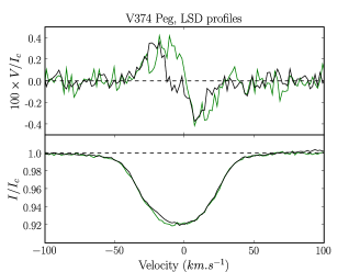
Figure 1: Typical examples of LSD Stokes $V$ and $I$ profiles of V374 Peg (top and bottom curves respectively) on 2006 August 08 (green line) and 2006 August 10 (black line).

3 Modelling intensity profiles

3.1 Model description

We use Doppler Imaging (DI) to convert time-resolved series of Stokes $I$ LSD profiles into maps of cool spots at the surface of V374 Peg. Thanks to the Doppler effect, cool spots on the photosphere of a rapidly rotating star produce profile distorsions in spectral lines whose locations strongly correlate with the spatial positions of the parent spots; in this respect, spectral lines of a spotted star can be viewed as one-dimensional (1D) image, resolved in the direction perpendicular to both the stellar rotation axis and the line of sight. By looking at how these 1D maps are periodically modulated as the star rotates enables one to recover a 2D map of the stellar photosphere (e.g., Vogt et al., 1987). Since this inversion problem is partly ill-posed, one needs to implement additional constraints to stabilise the imaging process, e.g., by selecting the image having the lowest information content using the maximum entropy algorithm of Skilling & Bryan (1984). More details about the principles and performance DI can be found in Vogt et al. (1987).

We implement this imaging process by dividing the surface of the star into a grid of 3,000 elementary cells. We describe the local line profile at each grid point of the stellar surface with the 2-component model of Cameron (1992), i.e., as a linear combination between two reference profiles, one representing the quiet photosphere (at temperature $T_{\rm q}$) and one representing cool spots (at temperature $T_{\rm s}$), both Doppler shifted by the local line-of-sight rotation velocity of the corresponding grid cell. The image quantity we reconstruct is the local spottedness at the surface of the star, i.e., the amount by which both reference profiles are mixed together, varying between 0 (no spot) and 1 (spots only). The algorithm aims at reconstructing the image with minimum spot coverage at the surface of the star, given a certain quality of the fit to the data.

More specifically, we assume that both reference profiles are equal and only differ by their relative continuum levels (set to their respective blackbody fluxes at the mean line wavelength). We further assume $\hbox{$T_{\rm q}$}=3200$ K (i.e., a typical surface temperature for a M4 star) and $\hbox{$T_{\rm s}$}=2800$ K (i.e., a low spot-to-photosphere temperature contrast in agreement with the findings of Berdyugina 2005). For the assumed reference profile, we can use either the LSD profile of the very slowly rotating inactive M dwarf Gl 402 (Delfosse et al., 1998), or a simple gaussian profile with similar full-width-at-half-maximum (FWHM, set to 9.25 km s^-1 including instrumental broadening) and equivalent width. Both options yield very similar results, demonstrating that the exact shape of the assumed local profile has very minor impact on the reconstructed images, as long as the projected rotation velocity of the star is much larger than the local profile. We further assume that continuum limb-darkening varies linearly with the cosine of the limb angle (with a slope of $u=0.6964$, Claret 2004); using a quadratic (rather than linear) dependence produces no visible change in the result.

The angle $i$ of the stellar rotation axis to the line-of-sight is taken to be $70\hbox{${}^{\circ}$}$ (e. g., D06). Given the projected equatorial velocity $v\sin i$ of V374 Peg (about 36.5 km s^-1, see below) and the width of the local profile (9.25 km s^-1, see above), the number of spatially resolved elements across the equator of the star is about 25, which is equivalent to a longitude resolution of 15^∘ or 0.04 rotation cycle. Using 3,000 grid cells at the surface of the star (112 across the equator) is therefore perfectly adequate for our needs.

3.2 Results

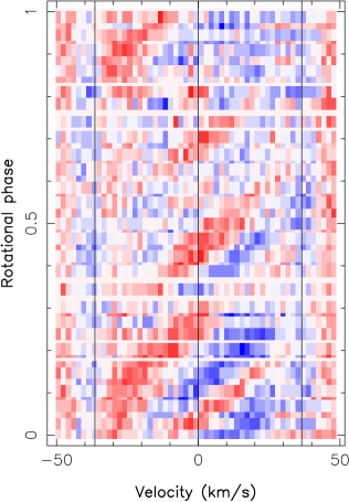
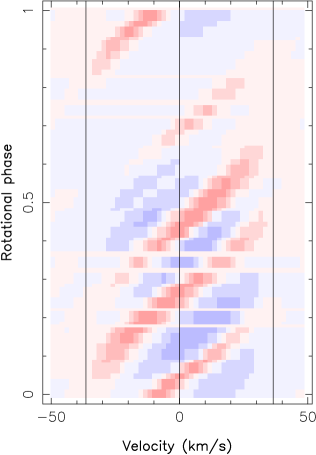
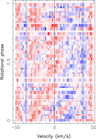
Figure 2: Observed (left), modelled (middle) and residual (right) Stokes $I$ dynamic spectra of V374 Peg for the Aug05 data set (60 spectra). A purely rotational profile is subtracted from all spectra to emphasize the image contrast. The fit corresponds to a S/N level of $700$. The colour scale ranges from –0.5% to 0.5% of the continuum level, red and blue respectively standing for a lack and an excess of absorption with respect to the synthetic purely rotationnal profile.

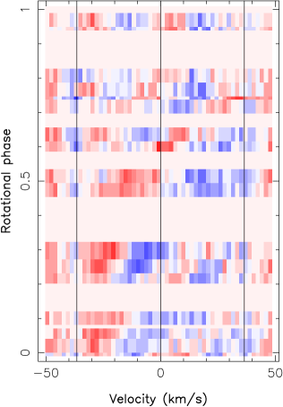
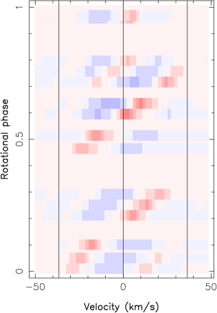
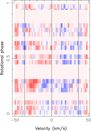
Figure 3: Same as Fig. 2 for the Aug06 data set (21 spectra).

       

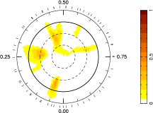
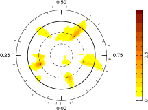
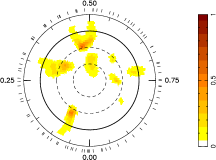
Figure 4: Doppler maps of the spottedness at the surface of V374 Peg reconstruct, as derived from the Aug05 (left panel) and Aug06 (middle panel) data sets. The last image (right) was recovered from the complete dataset (Aug05, Sep05, and Aug06 altogether), it represents the starspots configuration at an intermediate epoch (cycle 194) and takes into account the adjustment of the period and the inclusion of differential rotation (see Sec. 5). The star is shown in flattened polar projection down to latitudes of $-30\hbox{${}^{\circ}$}$, with the equator depicted as a bold circle and parallels as dashed circles. Radial ticks around each plot indicate phases of observations.

DI is very sensitive to the assumed $v\sin i$ (e.g., Vogt et al., 1987); small errors are known to generate specific belt-like artifacts around the stellar equator in the reconstructed image. We derive the optimum $v\sin i$ by minimising the reconstructed spot coverage at a given reduced chi-square (hereafter $\chi^{2}_{r}$) fit to the data, and find values of $36.5\pm 0.4$ km s^-1 and $36.7\pm 0.4$ km s^-1 for the Aug05 and Aug06 data sets respectively, when using the gaussian local profile model. Slightly different values (all lying with 0.5 km s^-1 of the previous estimates) are obtained when using the LSD profile of Gl 402 as local profile, or when using different models of the continuum limb darkening. Taking into account all potential sources of systematic errors, we obtain that the absolute accuracy to which $v\sin i$ is determined is about 1 km s^-1; in the following, we assume $\hbox{$v\sin i$}=36.5$ km s^-1.

Aug05 and Aug06 datasets can be fitted at S/N levels of 715 and 800 respectively. In particular, the distorsions travelling from the blue to the red profile wing are well reproduced (see Fig. 2 and 3). We note small systematic residual discrepancies between the observed and modelled profiles, showing up as vertical bands in the far line wings (see Fig. 2 and 3). These differences cannot be removed by adjusting $v\sin i$ or $u$ and do not affect the imaging of starspots. Another residual discrepancy is visible in the blue profile wing around phase 0.27 in the Aug06 data set (see Fig. 3, right panel). This discrepancy corresponds to a feature visible in the blue wing of the observed profiles (see Fig. 3, left panel), that the imaging code did apparently not convert into a starspot. The reason for this is that the code assumes the rotating star to host starspots exhibiting no intrinsic variability; if the observed (unfitted) feature was due to such a starspot, we would expect a similar signature to show up in the red wing of the observed profiles around phase 0.5, i.e., when the putative spot has reached the receding stellar limb. Since this is not the case here, we speculate that the residual unfitted spectral feature is either caused by a small flare or by an intrinsically variable starspot.

Both datasets yield spot occupancies of about 2% of the overall photosphere at both epochs. This rather low spottedness directly reflects the fact that distortions of unpolarised line profiles are rather small. Note that only spots (or spot groups) with sizes comparable to or larger than the resolution element can be reconstructed with DI, tiny isolated spots much smaller than our spatial resolution threshold remaining out of reach. The resulting brightness maps are shown in Fig. 4. While both maps are roughly similar, they apparently differ by more than a simple phase shift (that could result from a small error in the rotation period). Note that no obvious polar spot is reconstructed on V374 Peg. This result is quite reliable; since V374 Peg is a fast rotator, any strong polar structure would produce a clear distortion in the core of the Stokes $I$ profiles, giving them an obvious flat-bottom shape. This is not the case here, as one can see on Fig. 2

Small changes in $v\sin i$ (within 0.5 km s^-1), in the inclination angle (within 10^∘), in the local profile model (see above) or in the limb-darkening model (linear vs quadratic) produce negligible modifications in the reconstructed spot distributions.

4 Modelling circularly polarised profiles

4.1 Model description

We use Zeeman-Doppler Imaging (ZDI) to turn our series of rotationally modulated circularly-polarised LSD profiles into magnetic field maps at the surface of V374 Peg. ZDI is based on the same basic principles as DI except that it aims at mapping a vector field. The overall characteristics of the model we use are given below.

The vector magnetic field at the surface of the star is described using spherical harmonics expansions for each of the field component in spherical coordinates (e.g., Donati et al., 2001, 2006). Note that this is different from the initial ZDI attempts (e.g., Brown et al., 1991; Donati et al., 1997) in which the field was described as a set of independent pixels, containing the components of the field in each surface grid cell. The main advantage of this new method is that it straightforwardly allows the recovery of a physically meaningfull magnetic field, that we can easily split into its poloidal and toroidal components. This is of obvious interest for all studies on stellar dynamos. Another important point is that this new method is very successfull at recovering simple magnetic field structures such as dipoles (even from Stokes $V$ data sets only), while the old one reportedly failed at such tasks (Brown et al., 1991; Donati et al., 2001).

As for DI (see Sec. 3.1), the stellar surface is divided into a grid of 3 000 pixels on which the magnetic field components are computed from the coefficients of the spherical harmonics expansion. The contribution of each grid point to the synthetic Stokes $V$ spectra are derived using the weak-field approximation:

$$V(\lambda)=-g\frac{\lambda_{\rm 0}^{2}e}{4\pi m^{2}}B_{\rm\ell}\frac{dI}{d\lambda}$$ (2)

where $I$ is the local unpolarised profile (modelled with the same gaussian profile as in Sec. 3.1), $g$ and $\lambda_{\rm 0}$ the Landé factor and the centre rest wavelength of the average LSD line (set to 1.2 and 700 nm respectively), $e$ and $m$ the electron charge and mass respectively, and $B_{\rm\ell}$ the line-of-sight projection of the local magnetic field vector. Despite being an approximation, this expression is valid for magnetic splittings significantly smaller than the local profile width (prior to instrumental broadening); given that 2 kG fields yield Zeeman splittings of only about 2.5 km s^-1 in the case of our average LSD profile (i.e., about twice smaller than the FWHM of the local profile prior to instrumental broadening), this expression turns out to be accurate enough for our needs. This is further confirmed by using model local profiles computed from Unno-Rachkovsky’s equations, with which almost identical results are obtained.

As for DI, the inversion problem is partly ill-posed. We make the solution unique by introducing an entropy function describing the amount of information in the reconstructed image, and by looking for the image with maximum entropy (minimum information) among all those fitting the data at a given $\chi^{2}_{r}$ level. The entropy is now computed from the sets of complex spherical harmonics coefficients, rather than from the individual image pixels as before. We chose one of the simplest possible form for the entropy:

$$S=-\sum_{\ell,m}\ell\left(\alpha_{\ell,m}^{2}+\beta_{\ell,m}^{2}+\gamma_{\ell,m}^{2}\right)$$ (3)

where $\alpha_{\ell,m}$, $\beta_{\ell,m}$, $\gamma_{\ell,m}$ are the spherical harmonics coefficient of order $(\ell,m)$ describing respectively the radial, non-radial poloidal and toroidal field components. More detail about the process can be found in Donati et al. (2006). In particular, this function allows for negative values of the magnetic field (as opposed to the conventional expression of the Shannon entropy). The precise form of entropy (e.g., the multiplying factor $\ell$) has only minor impact on the resulting image.

As mentioned in in Sec. 3.1, the number of resolved elements on the equator is about 25, indicating that limiting the spherical harmonics expansion describing the magnetic field to orders lower than 25 should be enough and generate no loss of information. In practice, no significant change of the reconstructed image is observed when limiting the expansion at orders $\leq 10$. All results presented below are obtained assuming $\ell\leq 10$.

4.2 Results

We present here the results concerning the Aug05 dataset, though already reported in D06, in order to clarify the comparison with the Aug06 observations. The Aug05 data set can be fitted with a purely poloidal field down to $\hbox{$\chi^{2}_{r}$}=1.1$ (see Fig. 5 for the observed and modelled dynamic spectra at this epoch). No improvement to the fit is obtained when assuming that the field also features a toroidal component. We therefore conclude that the field of V374 Peg is mostly potential in Aug05 and that the toroidal component (if any) includes less than 4% of the overall large-scale magnetic field energy. The field we recover is shown in Fig. 7 (left column) while the corresponding spherical harmonics power spectra are shown in Fig. 8 (left column). The reconstructed large-scale field is found to be mostly axisymmetric, with the visible hemisphere being mostly covered with positive radial field (i.e., with radial field lines emerging from the surface of the star). As obvious from Fig. 8, the dominant mode we recover corresponds to $\ell=1$ and $m=0$ (i.e., a dipole field aligned with the rotation axis) and has an amplitude of about 2 kG; all other modes have amplitudes lower than 1 kG. The maximum field strength at the surface of the star reaches 1.3 kG, while the average field strength is about 0.8 kG.

Similar results are obtained from the Aug06 data, for which the observed spectra are fitted down to $\hbox{$\chi^{2}_{r}$}=1.0$ (see Fig. 6). Again, we find that the field is mostly axisymmetric, with 80% of the reconstructed magnetic energy concentrating in $m=0$ modes. The radial field component clearly dominates (75% of the energy content) while the toroidal component is once more very marginal (4% of the energy content). The main excited mode again corresponds to $\ell=1$ and $m=0$, features an amplitude of 1.9 kG and encloses as much as 60% of the overall magnetic energy content. The maximum and average field strengths recovered at the surface of the star are 1.2 kG and 0.7 kG respectively.

As a result of the limited spatial resolution of the imaging process, small-scale magnetic regions at the surface of V374 Peg are out of reach of ZDI. We can therefore not evaluate the amount of magnetic energy stored at small scales and compare it to that we recover at medium and large scales. We can however claim that scales corresponding to spherical harmonics orders ranging from about 5 to 25, to which our imaging process is sensitive, contain very little magnetic energy with respect to the largest scales ($\ell\leq 5$).

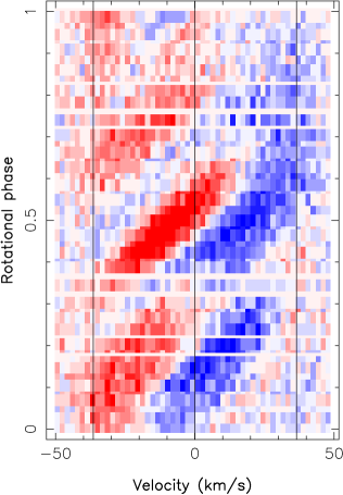
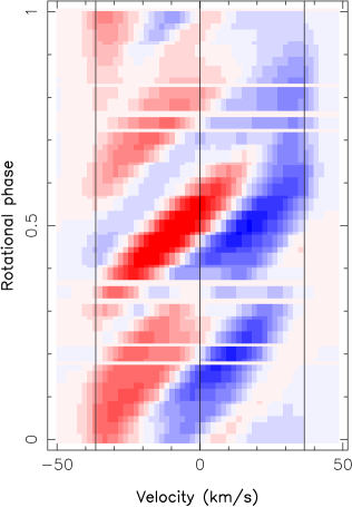
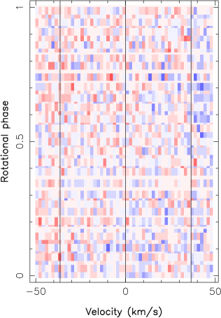
Figure 5: Observed (left), modelled (middle) and residual (right) Stokes $V$ dynamic spectra of V374 Peg for the Aug05 data set (60 spectra). The fit corresponds to $\hbox{$\chi^{2}_{r}$}=1.1$. The colour scale ranges from –0.4% to 0.4% of the continuum level, red and blue respectively standing for positive and negative circular polarization signal.

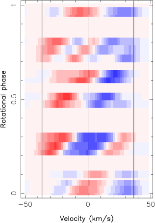
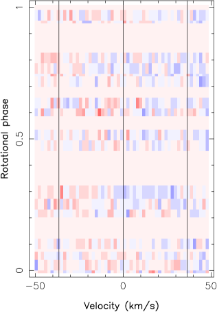
Figure 6: Same as Fig. 5 for the Aug06 data set (21 spectra). The fit corresponds to $\hbox{$\chi^{2}_{r}$}=1.0$.

We can also note that that the magnetic maps recovered from the Aug05 and Aug06 data sets are fairly similar apart from a 36^∘ (0.1 rotation cycle) global shift between both epochs, certainly resulting from a small error in the rotation period. Slight intrinsic differences also seem to be present, e.g., in the exact shape of the positive radial field distribution over the visible hemisphere. A straightforward visual comparison of both images is however not sufficient to distinguish whether these apparent discrepancies simply result from differences in phase coverage at both epochs, or truly reveal intrinsic variability of the magnetic topology between our two observing runs. To test this, one way is to merge all available data (including those collected in Sep05) in a single data set and to attempt fitting them with a single magnetic structure (and a revised rotation period). This is done in Sec. 5. In the meantime, we can nevertheless conclude that the magnetic topology of V374 Peg remained globally stable over a timescale of 1 yr.

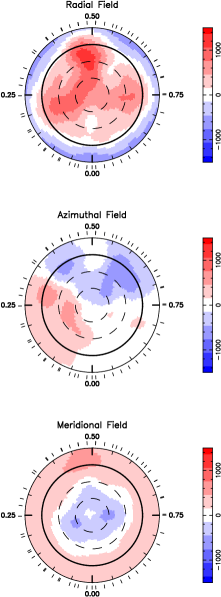
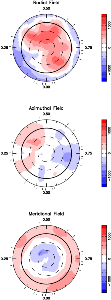
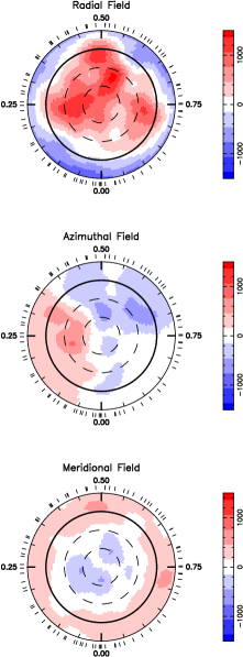
Figure 7: Surface magnetic field of V374 Peg as derived from our Aug05 (left) and Aug06 (middle) datasets. The last image (right) was recovered from the complete dataset (Aug05, Sep05, and Aug06 altogether), it represents the magnetic configuration at an intermediate epoch (cycle 194) and takes into account the adjustment of the period and the inclusion of differential rotation (see Sec. 5). The three components of the field in spherical coordinates are displayed from top to bottom (flux values labelled in G). The star is shown in flattened polar projection down to latitudes of $-30\hbox{${}^{\circ}$}$, with the equator depicted as a bold circle and parallels as dashed circles. Radial ticks around each plot indicate phases of observations.

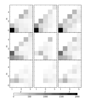
Figure 8: Spherical-harmonics power spectra of the magnetic field maps derived from our Aug05 (left), Aug06 (middle) and complete (right) data sets (magnetic fluxes labelled in G) after adjustment of the period and inclusion of differential rotation (see Sec. 5). From top to bottom, the magnetic power spectra respectively correspond to the radial poloidal, the non-radial poloidal and the toroidal field components. Only modes up to order 5 are plotted here (larger order modes containing very little power).

5 Differential Rotation and Magnetic field time-stability

To estimate the degree at which the magnetic topology remained stable over 1 yr, we merge all data together (Aug05, Sep05 and Aug06 datasets) and try to fit them simultaneously with a single field structure. We also assume that the surface of the star is rotating differentially (with a given differential rotation law, see below) over the complete period of our observations, and thus that the magnetic topology is slightly distorted as a result of this surface shear (with respect to the magnetic topology at median epoch, e. g. at cycle 194). If the fit to the complete data set is as good as that to both individual Aug05 and Aug06 data sets ($\hbox{$\chi^{2}_{r}$}\simeq 1$, see Sec. 4.2), it would demonstrate that no variability occurred (except that induced by differential rotation) over the full observing period. If, on the other hand, the fit quality to the complete data set is worse, it would indicate that intrinsic variability truly occurred, with the fit degradation directly informing on the actual level of variability.

To model differential rotation, we proceed as in Petit et al. (2002) and Donati et al. (2003), assuming that the rotation rate at the surface of the star is solar-like, i.e., that $\Omega$ varies with latitude $\theta$ as:

$$\Omega(\theta)=\hbox{$\Omega_{\rm eq}$}-\hbox{$d\Omega$}\sin^{2}\theta$$ (4)

where $\Omega_{\rm eq}$ is the rotation rate at the equator and $d\Omega$ the difference in rotation rate between the equator and the pole. We use this law to work out the phase shift of each surface grid cell, at any given epoch, with respect to its position at median epoch. These phase shifts are taken into account to compute the synthetic spectra corresponding to the current magnetic field distribution at all observing epochs using the model described in Sec. 4.1.

For each pair of $\Omega_{\rm eq}$ and $d\Omega$ values within a range of acceptable values (given by D06), we then derive, from the complete data set, the corresponding magnetic topology (at a given information content) and the associated $\chi^{2}_{r}$ level at which modelled spectra fit observations. By fitting a paraboloid to the $\chi^{2}_{r}$ surface derived in this process (Donati et al., 2003), we can easily infer the magnetic topology that yields the best fit to the data along with the corresponding differential rotation parameters and error bars.

The best fit we obtain corresponds to $\hbox{$\chi^{2}_{r}$}=1.15$, demonstrating that intrinsic variability between Aug05 and Aug06 remains very limited, as guessed in Sec. 4.2 by visually comparing the images from individual epochs. The derived $\chi^{2}_{r}$ map (see Fig. 9) features a clear paraboloid around the $\chi^{2}$ minimum, yielding differential rotation parameters at the surface of V374 Peg equal to $\hbox{$\Omega_{\rm eq}$}=14.09880\pm 0.00006$ rad d^-1 (corresponding to $P_{\rm rot}=0.445654\pm 0.000002$ d) and $\hbox{$d\Omega$}=0.0063\pm 0.0004$ rad d^-1. Due to the large time gap between the two main observing epochs (about 1yr), the $\chi^{2}_{r}$ map exhibits aliases on both left and right sides of the minimum, corresponding to shifts of $\sim 6\times 10^{-4}$ d on $P_{\rm rot}$. The nearest local minima, located at $\hbox{$\Omega_{\rm eq}$}=14.08110$ rad d^-1 and $\hbox{$\Omega_{\rm eq}$}=14.11664$ rad d^-1, are associated with $\chi^{2}_{r}$ values of 1.27 and 1.30 respectively, i.e., to $\Delta\hbox{$\chi^{2}$}$ values of 600 and 740 respectively; the corresponding rotation rates can thus be safely excluded.

In addition to refining the rotation period (error bar shrunk by 2 orders of magnitude with respect to D06), we also detect a small but definite surface shear, about 10 times weaker than that of the Sun. Assuming solid body rotation does not allow to reach $\chi^{2}_{r}$ levels below 1.5; this unambiguously demonstrates that the surface of V374 Peg is not rotating as a solid body and is truly twisted by differential rotation. The reconstructed magnetic map along with the corresponding spherical-harmonics power spectra are shown in the right panels of Figs. 7 and 8.

The same procedure is used on Stokes $I$ data. However, the $\chi^{2}_{r}$ map we obtain does not feature a clear paraboloid, but rather a long valley with no spatially well-defined minimum; this is not unexpected given the fact that spots reconstructed at the surface of V374 Peg do not span a wide range of latitudes (as requested for a clean differential rotation measurement, see Petit et al. 2002) but rather concentrate at low latitudes. Using the differential rotation parameters derived from Stokes $V$ data yields a fit corresponding to a S/N level of about 680, i.e., only slightly lower than that achieved at each individual epoch (see Sec. 3.2). It suggests that only moderate intrinsic variability occurred in the brightness distribution as well, despite the apparent (but weakly significant) differences between the two individual images. The corresponding image (reconstructed from the full data set) is shown in Fig. 4 (right panel).

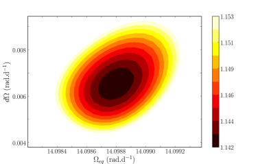
Figure 9: Variation of $\chi^{2}_{r}$ as a function of the differential rotation parameters $\Omega_{\rm eq}$ and $d\Omega$. The last colour contour corresponds to a $\chi^{2}_{r}$ increase of 1%, i.e., to an error bar of about 7$\sigma$ (for each parameter taken separately).

6 Chromospheric Activity

We compute the mean and standard deviation profiles of the H$\alpha$, H$\beta$ and Ca ii infrared triplet (IRT) lines. Both H$\alpha$ and H$\beta$ lines are in strong emission whereas the infrared triplet is observed mostly in absorption with sporadic emission episodes (due to flares). We notice that, for all studied lines, variability concentrates within $\pm\hbox{$v\sin i$}$ about the line centre (see Fig. 10), suggesting that activity is mostly located close to the surface.

For each observation, we compute the emission equivalent width of the chromospheric lines. The result for H$\alpha$ is plotted on Fig. 11 as a function of rotational phase, H$\beta$ and Ca ii IRT exhibiting a very similar behaviour. We first conclude that all three lines do not undergo pure rotational modulation, sometimes displaying very different emission levels at similar phases of successive rotation cycles (e.g., phase 0.2, see Fig. 11). We attribute the basal emission component (in Balmer lines) to quiescent activity and the intrinsically variable emission component to flares.

Maximum flaring activity is observed around phases 0.20 and 0.75–1.00, but also, to a lesser extend at phases 0.50–0.60 (see Fig. 11, bottom panel). Note that the four photospheric profiles discarded from our imaging analysis (see Sec. 2) were collected on 2005 August 21 at phases 0.72 and 0.78 and on 2005 August 23 at phases 0.19 and 0.23, i.e., at the very beginning of the two main flaring episodes we recorded.

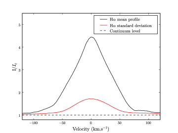
Figure 10: H$\alpha$ mean profile (black solid line) and standard deviation (red solid line, shifted by $+1$), along with continuum level (dashed line). All profiles are shown in the stellar velocity rest frame.

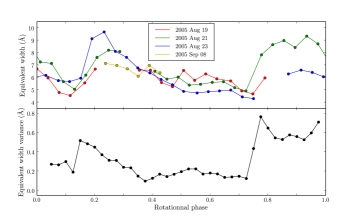
Figure 11: Emission equivalent width of H$\alpha$ as a function of the rotational phase in Aug05 and Sep05, consecutive observations are linked together by a solid line (top panel); along with associated standard deviation (computed over phase intervals of 0.1 cycle, bottom panel).

7 Discussion and conclusion

Spectropolarimetric observations of V374 Peg were carried out with ESPaDOnS and CFHT at 3 epochs over a full time span of about 1 yr. Clear Zeeman signatures are detected in most Stokes $V$ spectra; weak distortions are also observed in the unpolarised profile of photospheric lines.

Using DI, we find that only a few low-contrast spots are present at the surface of V374 Peg, covering altogether 2% of the overall surface. The spot distribution is apparently variable on a timescale of 1 yr. Even though we may be missing small spots evenly peppering the photosphere (e.g., Jeffers et al., 2006), V374 Peg nevertheless appears as fairly different from warmer, partly-convective, active stars, whose surfaces generally host large, high-contrast cool spots often covering most of the polar regions at rotation rates as high as that of V374 Peg (e.g., Donati et al., 2000). Barnes et al. (2004) also report the lack of a cool polar structure for the M1.5 – largely but not fully convective – fast rotator HK Aqr ($\hbox{$P_{\rm rot}$}=0.431$ d). A spot occupancy of about 2% has been observed for very slow rotators as well (Bonfils et al., 2007; Demory et al., 2007), suggesting that spot coverage may not correlate with rotation rate in M dwarfs, as oppposed to what is observed in hotter stars (e. g., Hall, 1991).

Using ZDI, we find that the surface magnetic topology of V374 Peg is mostly poloidal and fairly simple, with most of the energy concentrating within the lowest-order axisymmetric modes. This confirms and amplifies the previous results of D06. Again, this is at odds with surface magnetic topologies of warmer active stars, usually showing strong and often dominant toroidal field components in the form of azimuthal field rings more or less encircling the rotation axes (e.g., Donati et al., 2003). As for surface spots, ZDI is mostly insensitive to small-scale magnetic regions (and in particular small-scale bipoles) that can also be present at the surface of V374 Peg; we can however claim that very little magnetic energy concentrates in spherical-harmonic terms with $\ell$ ranging from 5 to 25.

We find that the surface magnetic topologies of V374 Peg at epoch Aug05 and Aug06 are very similar apart from an overall shift of about 0.1 rotation cycle. This is confirmed by our success at fitting the complete Stokes $V$ data set down to almost noise level with a unique magnetic field topology twisted by a very small amount of solar-like differential rotation. It suggests in particular that magnetic topologies of fully-convective stars are globally stable on timescales of at least 1 yr. Again, this is highly unusual compared to the case of warmer active stars, whose detailed magnetic topologies evolve beyond recognition in timescales of only a few weeks (e.g., Donati et al., 2003).

The updated rotation period and photospheric shear we find for V374 Peg are respectively equal to $0.445654\pm 0.000002$ d and $0.0063\pm 0.0004$ rad d^-1respectively; the corresponding time for the equator to lap the pole by one complete rotation cycle is equal to 2.7 yr, about 10 times longer than solar. We speculate that this unusually small differential rotation and long lap time are in direct relationship with the long lifetime of the magnetic topology, suggesting that differential rotation is what mostly controls the lifetime of magnetic topologies. New data collected on a smaller time span (a few months) and featuring in particular no intrinsic variability (other than that generated by differential rotation) are needed to provide an independent and definite confirmation of this result.

Although the spot distributions at the surface of V374 Peg at epoch Aug05 and Aug06 apparently differ from more than a simple phase shift of 0.1 cycle, both data sets are compatible with a unique brightness map undergoing moderate intrinsic variability (assuming differential rotation is similar to that derived from Stokes $V$ data). The low spottedness level and weak spot contrast implies that densely sampled data sets at 2 nearby epochs are needed to confirm this result, derive an independent determination of differential rotation parameters from unpolarised spectra and check that spots and magnetic fields trace the same atmospheric layers.

The strong mostly-axisymmetric poloidal field of V374 Peg can hardly be reconciled with the very weak level of surface differential rotation in the context of the most recent dynamo models of fully-convective stars. While Dobler et al. (2006) predicts that rapidly-rotating fully-convective stars should be able to sustain strong poloidal axisymmetric fields with the help of significant (though antisolar) differential rotation, Chabrier & Küker (2006) find that these stars should only be able to trigger purely non-axisymmetric magnetic topologies if differential rotation is lacking (or remains below a threshold of about 1/3 of the solar value, Chabrier, private communication). Both findings are at odds with our observational results, suggesting that our theoretical understanding of dynamo action in fully-convective stars is still incomplete.

We report the detection of strong chromospheric activity in V374 Peg, including quiescent emission in Balmer lines along with sporadic flaring events in H$\alpha$, H$\beta$ and the Ca ii IRT. This is noticeably different from what was recently reported by Berger et al. (2007) for the M8.5 brown dwarf TVLM 513-46546, whose rotationally modulated H$\alpha$ emission identically repeats over several successive rotation cycles. From the width and variability of emission profiles, we conclude that activity occurs mostly close to the stellar surface on V374 Peg, with flares apparently concentrating at specific longitudes. However, there is no clear spatial correlation between the photospheric magnetic field, the starspots and these chromospheric regions, e.g., strongest magnetic fields being observed when chromospheric activity is low. Simultaneous multiwavelength observations of V374 Peg, including in particular optical spectropolarimetry, X-ray, and radio monitoring, could allow us to investigate the 3D magnetosphere of fully convective stars (e.g., by extrapolating the photospheric field topology up to the corona), and to unravel how photospheric activity relates to chromospheric and coronal activity.

Finally, we note that our $v\sin i$ and rotation period estimates imply that $\hbox{$R_{\star}$}\sin i=0.32\pm 0.01$ ${\rm R}_{\odot}$, and thus that $\hbox{$R_{\star}$}\simeq 0.34$ ${\rm R}_{\odot}$ (assuming $i\simeq 70\hbox{${}^{\circ}$}$). Given the $M_{\rm K}$ magnitude of V374 Peg (equal to $7.0\pm 0.3$), we can safely derive that V374 Peg has a mass of $0.28\pm 0.05$ ${\rm M}_{\odot}$ (Delfosse et al., 2000). It implies that the radius of V374 Peg is slightly larger than what theoretical models predict for low-mass stars of similar masses. Ribas (2006) also reports stellar radii larger than the theoretical predictions for very-low mass eclipsing binaries (whose rotation period is very short), whereas the radii of slowly rotating M dwarfs match the predicted values (e. g., Ségransan et al., 2003). According to the phenomenological model of Chabrier et al. (2007) the presence of a strong magnetic field may inhibit stellar convection and therefore lead to larger radii with respect to an inactive star of equal mass.

Future observations are thus needed to explore in more details the magnetic topologies, brightness distributions and differential rotation of V374 Peg and other fully-convective stars. Finding out how these quantities vary with mass and rotation rate could in particular show us the way to more successfull simulations of dynamo processes in low-mass fully-convective stars.

References

- Barnes et al. (2005) Barnes J. R., Cameron A. C., Donati J.-F., James D. J., Marsden S. C., Petit P., 2005, MNRAS, 357, L1
- Barnes et al. (2004) Barnes J. R., James D. J., Cameron A. C., 2004, MNRAS, 352, 589
- Berdyugina (2005) Berdyugina S. V., 2005, Living Reviews in Solar Physics, 2, 8
- Berger et al. (2007) Berger E., Gizis J. E., Giampapa M. S., Rutledge R. E., Liebert J., Martin E., Basri G., Fleming T. A., Johns-Krull C. M., Phan-Bao N., Sherry W. H., , 2007, arXiv:0708.1511
- Bonfils et al. (2007) Bonfils X., Mayor M., Delfosse X., Forveille T., Gillon M., Perrier C., Udry S., Bouchy F., Lovis C., Pepe F., Queloz D., Santos N. C., Bertaux J. L., , 2007, arXiv:0704.0270
- Brown et al. (1991) Brown S. F., Donati J.-F., Rees D. E., Semel M., 1991, A&A, 250, 463
- Cameron (1992) Cameron A., 1992, in Byrne P. B., Mullan D. J., eds, Surface Inhomogeneities on Late-Type Stars Vol. 397 of Lecture Notes in Physics, Berlin Springer Verlag, Modelling Stellar Photospheric Spots Using Spectroscopy (Invited). p. 33
- Chabrier & Baraffe (1997) Chabrier G., Baraffe I., 1997, A&A, 327, 1039
- Chabrier et al. (2007) Chabrier G., Gallardo J., Baraffe I., , 2007, Evolution of low-mass star and brown dwarf eclipsing binaries
- Chabrier & Küker (2006) Chabrier G., Küker M., 2006, A&A, 446, 1027
- Claret (2004) Claret A., 2004, A&A, 428, 1001
- Delfosse et al. (1998) Delfosse X., Forveille T., Perrier C., Mayor M., 1998, A&A, 331, 581
- Delfosse et al. (2000) Delfosse X., Forveille T., Ségransan D., Beuzit J.-L., Udry S., Perrier C., Mayor M., 2000, A&A, 364, 217
- Demory et al. (2007) Demory B. O., Gillon M., Barman T., Bonfils X., Mayor M., Mazeh T., Pont F., Queloz D., Udry S., Bouchy F., Delfosse X., Forveille T., Mallmann F., Pepe F., Perrier C., , 2007, Characterization of the hot Neptune GJ 436b with Spitzer and ground-based observations
- Dobler et al. (2006) Dobler W., Stix M., Brandenburg A., 2006, ApJ, 638, 336
- Donati et al. (2003) Donati J.-F., Cameron A., Semel M., Hussain G., Petit P., Carter B., Marsden S., Mengel M., Lopez Ariste A., Jeffers S., Rees D., 2003, MNRAS, 345, 1145
- Donati et al. (2006) Donati J.-F., Catala C., Landstreet J. D., Petit P., 2006, in Casini R., Lites B. W., eds, Astronomical Society of the Pacific Conference Series Vol. 358 of Astronomical Society of the Pacific Conference Series, ESPaDOnS: The New Generation Stellar Spectro-Polarimeter. Performances and First Results. p. 362
- Donati et al. (2003) Donati J.-F., Collier Cameron A., Petit P., 2003, MNRAS, 345, 1187
- Donati et al. (2006) Donati J.-F., Forveille T., Cameron A. C., Barnes J. R., Delfosse X., Jardine M. M., Valenti J. A., 2006, Science, 311, 633
- Donati et al. (2006) Donati J.-F., Howarth I. D., Jardine M. M., Petit P., Catala C., Landstreet J. D., Bouret J.-C., Alecian E., Barnes J. R., Forveille T., Paletou F., Manset N., 2006, MNRAS, 370, 629
- Donati et al. (2000) Donati J.-F., Mengel M., Carter B., Marsden S., Cameron A., Wichmann R., 2000, MNRAS, 316, 699
- Donati et al. (1997) Donati J.-F., Semel M., Carter B. D., Rees D. E., Cameron A. C., 1997, MNRAS, 291, 658
- Donati et al. (2001) Donati J.-F., Wade G., Babel J., Henrichs H., de Jong J., Harries T., 2001, MNRAS, 326, 1256
- Durney et al. (1993) Durney B. R., De Young D. S., Roxburgh I. W., 1993, Solar Physics, 145, 207
- Hall (1991) Hall D. S., 1991, in Tuominen I., Moss D., Rüdiger G., eds, IAU Colloq. 130: The Sun and Cool Stars. Activity, Magnetism, Dynamos Vol. 380 of Lecture Notes in Physics, Berlin Springer Verlag, Learning about stellar dynamos from long-term photometry of starspots. pp 353–+
- Jeffers et al. (2006) Jeffers S., Barnes J., Cameron A., Donati J.-F., 2006, MNRAS, 366, 667
- Johns-Krull & Valenti (1996) Johns-Krull C. M., Valenti J. A., 1996, ApJ, 459, L95+
- Küker & Rüdiger (2005) Küker M., Rüdiger G., 2005, Astronomische Nachrichten, 326, 265
- Kurucz (1993) Kurucz R., 1993, CDROM # 13 (ATLAS9 atmospheric models) and # 18 (ATLAS9 and SYNTHE routines, spectral line database). Smithsonian Astrophysical Observatory, Washington D.C.
- Petit et al. (2002) Petit P., Donati J.-F., Cameron A., 2002, MNRAS, 334, 374
- Reiners & Basri (2007) Reiners A., Basri G., 2007, ApJ, 656, 1121
- Ribas (2006) Ribas I., 2006, Ap&SS, 304, 89
- Saar & Linsky (1985) Saar S. H., Linsky J. L., 1985, ApJ, 299, L47
- Ségransan et al. (2003) Ségransan D., Kervella P., Forveille T., Queloz D., 2003, A&A, 397, L5
- Skilling & Bryan (1984) Skilling J., Bryan R. K., 1984, MNRAS, 211, 111
- Vogt et al. (1987) Vogt S. S., Penrod G. D., Hatzes A. P., 1987, ApJ, 321, 496