Vibrational excitations in systems with correlated disorder

Abstract

We investigate a $d$-dimensional model ($d$ = 2,3) for sound waves in a disordered environment, in which the local fluctuations of the elastic modulus are spatially correlated with a certain correlation length. The model is solved analytically by means of a field-theoretical effective-medium theory (self-consistent Born approximation) and numerically on a square lattice. As in the uncorrelated case the theory predicts an enhancement of the density of states over Debye’s $\omega^{d-1}$ law (“boson peak”) as a result of disorder. This anomay becomes reinforced for increasing correlation length $\xi$. The theory predicts that $\xi$ times the width of the Brillouin line should be a universal function of $\xi$ times the wavenumber. Such a scaling is found in the $2d$ simulation data, so that they can be represented in a universal plot. In the low-wavenumber regime, where the lattice structure is irrelevant there is excellent agreement between the simulation at small disorder. At larger disorder the continuum theory deviates from the lattice simulation data. It is argued that this is due to an instability of the model with stronger disorder.

I Introduction 

The influence of quenched disorder on the dynamic properties of solids is enormous and is subject to widespread experimental and theoretical investigations binder . The disorder leads to strong modifications of physical properties of the solid. On the other hand, the absence of lattice order in the solids and the corresponding breakdown of the Bloch theorem leads to appreciable difficulties for the theoretical interpretation of the disorder-induced phenomena. Here mean-field theories and particularly effective-medium theories have been of much help alexander , as they very often lead, at least, to a qualitative understanding of the influence of the disorder. In particular the coherent-potential approximation krumhansl (CPA) and its small-disorder version, the self-consistent Born approximation (SCBA) ballentine , have proved to be useful for interpreting the electronic and other spectral properties of disordered solids. In many cases physically different situations can be mapped onto each other. So one can convert an electronical problem to a vibrational one by replacing the energy $E$ by $-\omega^{2}$, where $\omega$ is the frequency parameter. If $E$ is replaced by $i\tilde{\omega}$, one studies the mathematical analogous diffusion problem alexander ; schirm01 ; schirm1 , where $\tilde{\omega}$ denotes the time Fourier parameter of the diffusion dynamics.

In the case of vibrational properties the disorder-induced excess in the density of states (DOS) over Debye’s $\omega^{d-1}$ law ($d$ is the dimensionality) (“boson peak”) has been successfully explained for a lattice model by comparing a simulation of a disordered lattice system with the predictions of the lattice CPA schirm0 . The comparison showed once more that the CPA is a reliable theory of disorder. In this study it was shown that the boson peak anomaly marks the crossover from plane-wave like vibrational states to disorder-dominated states with increasing frequency $\omega$. Near the crossover the effective sound velocity $v$ becomes complex and frequency dependent. This corresponds to a dc-ac crossover in the analogous diffusion problem schirm1 .

A similar but lattice-independent approach is the generalised elasticity theory in which the disorder is assumed to lead to spatial fluctuations of the elastic constants schirm2 . This model was solved by functional-integral techniques in which the SCBA plays the role of a saddle-point in a non-linear sigma-model treatment. This theory allowed for a generalization to include transverse degrees of freedom and to formulate a thermal transport theory schirm3 . Within this theory it was shown that the so-called plateau in the temperature dependence of the thermal conductivity freeman is caused by the boson-peak anomaly schirm3 . Furthermore, it has turned out schirm4 that the sound attenuation parameter (which is proportional to the imaginary part of $v(\omega)$) is related to the excess in the DOS in the boson peak regime.

It should be noted that the model of spatially fluctuating elastic constants, treated in CPA and SCBA is by no means the only approach for explaining the boson-peak anomaly. In fact, an enormous number of possible explanations have been published in the literature, which can roughly grouped into three classes: $i$) defect models, $ii$) models associated with the glass transition and $iii$) models with spatially fluctuating elastic constants.

$i$): Defects with a heavy mass can produce resonant quasi-local resonant states within the DOS economou ; burin ; polishchuk and be thus the reason for the boson peak and the reduction of the thermal conductivity. Similarly defects with very small elastic constants, near which anharmonic interactions are important (soft potentials), can produce quasi-local states, which, if hybridized with acoustic excitations may produce a boson peak soft ; gurevich and a plateau in the thermal conductivity buchenau ; gil Inhomongeneities may also be the source of local vibrational excitations that contribute to the excess DOS duval . Specifically in network glasses bond-angle distortions may also contribute to the boson-peak anomaly nucker ; nakayama . In a recent study schirm2 the predictions of a defect model has been compared with those of a fluctuating elastic constant model. $ii$): In theories of the glass transition gotzemayr ; chong ; xu ; lubchenko ; angell the boson peak arises as a benchmark of the frozen glassy state. $iii$) In models with quenched disorder of elastic constants schirm01 ; schirm1 ; taraskin ; parisi1 ; parisi2 ; bunde ; kuhn ; schirm2 ; schirm3 ; schirm4 the boson peak marks the lower frequency bound of a band of irregular delocalized states with random mutual hybridization. These states are neither propagating nor localized schirm0 . The models have been solved with the help of numerical simulations as well as effective-medium theories.

A drawback of these models is that they are based on the model assumption of uncorrelated disorder, i.e. spatial fluctuations of the physical quantities are assumed to be uncorrelated. This assumption is only justified if the spatial correlation length is smaller or of the order of the natural length which appears in the system under consideration. In the present problem, namely vibrations in disordered solids, there are two important length scales. One is just the interatomic distance $a$, the other is the sound velocity, divided by the boson-peak frequency, which is in experimental data of the order of several interatomic distances. The wavenumber corresponding to this length scale is the maximum wavenumber wich can serve as a label for wave-like vibrational states. In any case it is a more sound procedure to start with a theory with correlated disorder and make the approximation of short correlations (if appropriate) only in the end. Such theories are available john ; ignat ; bernhard . The aim of the present contribution is twofold: First we summarise the main features of the long-range-order SCBA. Secondly we present results of a two-dimensional simulation and compare them with those of the analytic theory.

II Model and self-consistent Born approximation (SCBA) 

We start with the equation of motion for scalar wave-like excitations $u({\bf r},t)$ in a $d$-dimensional disordered medium

$$\frac{\partial^{2}}{\partial t^{2}}\,u({\bf r},t)=\nabla\cdot\,v^{2}({\bf r})\,\cdot\nabla\,u({\bf r},t)$$ (1)

Here $v({\bf r})$ is a sound velocity (and $v^{2}({\bf r})$ an elastic constant), which is supposed to exhibit random spatial fluctuations $v^{2}({\bf r})=v_{0}^{2}+\Delta({\bf r})$ with $v_{0}^{2}=\langle v^{2}\rangle$ and

$$\langle\Delta({\bf r}+{\bf r}_{0})\Delta({\bf r}_{0})\rangle=C({\bf r})=\langle\Delta^{2}\rangle e^{-r/\xi}$$

$$\Leftrightarrow\quad \qquad C({\bf k})=\langle\Delta^{2}\rangle C_{0}\,[k^{2}+\xi^{-2}]^{-\frac{d+1}{2}}$$ (2)

with $C_{0}=2\pi(3d\!-\!5)/\xi$. In an effective-medium approximation the disordered system is mapped onto a homogeneous system, in which the influence of the disorder enters via a self-energy function $\Sigma({\bf k},z)$ with $z=\omega+i\epsilon$. The dynamic susceptibility is given by

$$\chi({\bf k},z)=\frac{k^{2}}{-z^{2}+k^{2}(v_{0}^{2}-\Sigma({\bf k},z))}$$ (3)

In SCBA the self-energy function obeys the self-consistent equation ballentine ; john ; ignat ; bernhard

$$\Sigma({\bf q},z)=\frac{1}{2}\int\limits_{|{\bf k}|<k_{D}}\left(\frac{\rm d{\bf k}}{2\pi}\right)^{d}C({\bf q}-{\bf k})\chi({\bf k},z)$$ (4)

with the Debye wavenumber $k_{D}=[2d\pi^{d-2}]^{1/2}/a$.

In the present study we are mainly interested in the low-frequency and -wavenumber properties, so we replace the self-energy by its $q\rightarrow 0$ limit $\Sigma(z)$ and obtain the SCBA equation

$$\!\Sigma(z)=\frac{\gamma}{2}\,\,{\textstyle\frac{v_{0}^{4}}{\varphi_{d}}}\!\!\!\int\limits_{|{\bf k}|<k_{D}}\!\!\!\!\left(\frac{{\rm d}{\bf k}}{2\pi}\right)^{d}\!\frac{k^{2}C(k)/\langle\Delta^{2}\rangle}{-z^{2}+k^{2}\left(v_{0}^{2}-\Sigma(z)\right)}$$ (5)

with the normalization constant $\varphi_{d}={\scriptstyle\!\!\!\!\int\limits_{|{\bf k}|<k_{D}}\!\!\!\!({\rm d}{\bf k}/2\pi)^{d}C({\bf k})/\langle\Delta^{2}\rangle}$ and the “disorder parameter” $\,\,\gamma=\langle\Delta^{2}\rangle\varphi_{d}/v_{0}^{4}$.

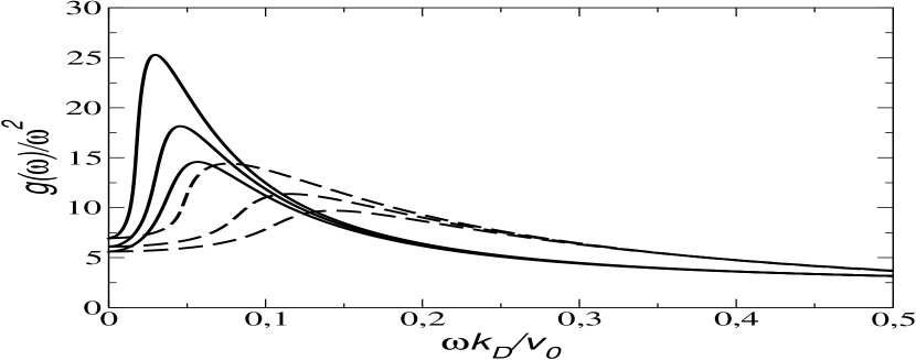
Figure 1: Reduced DOS $g(\omega)/\omega^{2}$ for $\xi\!=\!1/k_{D}$ (dashed lines) and $\xi\!=\!5/k_{D}$ (full lines) and for three disorder parameters (from left to right) $\gamma$ = 0.49, 0.47 and 0.45.

The DOS is given by

$$g(\omega)=\frac{2\omega}{\pi}{\rm Im}\left\{\int\left(\!\frac{\rm d{\bf k}}{2\pi}\right)^{d}\!\!\frac{1}{-z^{2}+k^{2}(v_{0}^{2}-\Sigma(z))}\right\}$$ (6)

In Fig. 1 we have plotted the “reduced DOS” $g(\omega)/\omega^{2}$ for $d=3$ and for three values of $\gamma$ and two values of $\xi$. First we notice that, as in the uncorrelated case schirm0 ; schirm2 ; schirm3 there exists a critical amount of disorder $\gamma_{c}=0.5$, beyond which the system becomes unstable. The “boson peak” becomes more pronounced and situated at lower frequencies as this value is approached. The interesting new feature in the correlated case is that the boson peak is re-inforced by the correlation and again shifted towards lower frequencies.

III Dynamic structure factor and density of states

We now divide the self-energy function into a real and imaginary part $\Sigma(z)\!=\!\Sigma^{\prime}(\omega\!\approx\!0)\!+\!i\Sigma^{\prime\prime}(\omega)$ and define the renormalised sound velocity as $v^{2}=v_{0}^{2}\!-\!\Sigma^{\prime}$. The dynamical structure factor $S({\bf k},\omega)$, which can be measured by inelastic neutron or X-ray scattering, and which is the Fourier transform of the dynamic density-density correlation function, is then given by the fluctuation-dissipation theorem hansen as

$$\qquad S(k,\omega)=\frac{k_{B}T}{\pi\omega}\mbox{Im}\left\{\chi(k,z)\right\}$$

$$\approx\frac{k_{B}T}{2\pi v^{2}}\frac{k^{2}\Sigma^{\prime\prime}(\omega)/2\omega}{\left[(kv-\omega)^{2}+(k^{2}\Sigma^{\prime\prime}(\omega)/2\omega)^{2}\right]}$$ (7)

The Brillouin resonance is given by $\omega=kv$ and the line width (FWHM, sound attenuation parameter) is given by

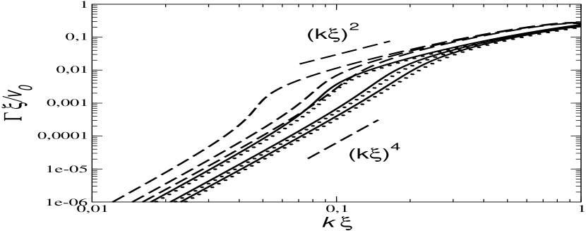
Figure 2: Scaled Brillouin linewidth $\Gamma\xi/v_{0}$ against scaled wavenumber $q\xi$ for $\xi\!=\!1/k_{D}$ (dashed lines) comment , $\xi\!=\!5/k_{D}$ (full lines), $\xi\!=\!10/k_{D}$ and $15/k_{D}$ (dotted lines). The disorder parameters $\gamma$ are the same as in Fig. 1.

$$\Gamma(k)=\frac{k}{v}\Sigma^{\prime\prime}(\omega=v\,k)$$ (8)

It can easily be shown that $\Sigma^{\prime\prime}\propto\omega^{d}$ for $\omega\rightarrow 0$ so that $\Gamma\propto q^{d+1}$ for $q\rightarrow 0$ (Rayleigh law).

We   now   introduce   the   dimensionless   variables $\tilde{\Sigma}\!=\!\Sigma/v_{0}^{2}\,$, $\,\,\tilde{C}_{0}=C_{0}\xi=2\pi(3d-5)$, $\,\,\tilde{z}\!=\!z\xi/v_{0}\!=\!\tilde{\omega}\!+\!i\tilde{\epsilon}$
and $\tilde{k}\!=\!k\xi$. We then obtain

$$\tilde{\Sigma}(\tilde{z})=\frac{\gamma}{2}\,\,{\textstyle\,\frac{\tilde{C}_{0}}{\varphi_{d}}}\!\!\!\!\int\limits_{|\tilde{\bf k}|<\xi k_{D}}\!\!\!\left(\frac{\rm d\tilde{\bf k}}{2\pi}\right)^{d}\!\frac{\!\tilde{k}^{2}\,[1+\tilde{k}^{2}]^{-(d+1)/2}}{-\tilde{z}^{2}+\tilde{k}^{2}(1-\tilde{\Sigma}(\tilde{z}))}$$ (9)

In this expression the correlation length $\xi$ enters only via the upper $\tilde{k}$ cutoff. For the limit $\xi\gg a$ we therefore obtain the scaling relation

$$\tilde{\Gamma}=\Gamma\xi/v_{0}=f(\gamma,\tilde{k})$$ (10)

In Fig. 2 we have plotted $\tilde{\Gamma}$ against $\tilde{k}$ for $d=3$, for the three $\gamma$ values of Fig. 1 and for $\xi$ = $1/k_{D}$, $5/k_{D}$, $10/k_{D}$, and $15/k_{D}$. We see that the scaling is obeyed except for $\xi=1/k_{D}$ comment as expected. As in the uncorrelated case schirm4 , the boson peak (see Fig. 1) marks the crossover from the Rayleigh regime $\tilde{\Gamma}\propto\tilde{k}^{4}$ to a behaviour $\tilde{\Gamma}\propto\tilde{k}^{s}$ with $s\approx 2$.

IV Simulation

We now discretize (1) in $d=2$ on a square lattice, which then takes the form of an equation of motion for unit masses connected by springs with spring constants $K_{ij}=\frac{1}{2a^{2}}(v^{2}(r_{i})+v^{2}(r_{j}))$:

$$\frac{{\rm d}^{2}}{{\rm d}t^{2}}\,u({\bf r}_{i},t)=\sum\limits_{\ell\,\,n.N.}K_{i\ell}[u({\bf r}_{\ell},t)-u({\bf r}_{i},t)]$$ (11)

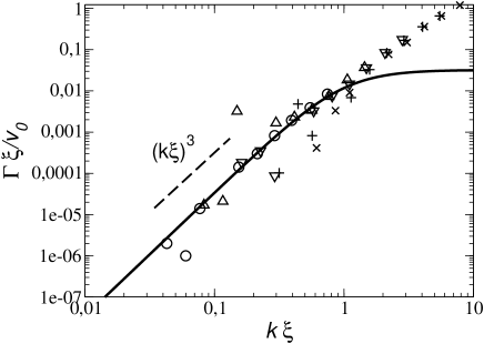
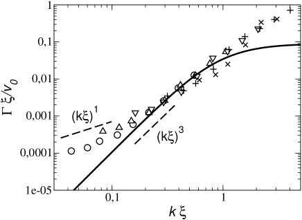
Figure 3: Symbols: Linewidths $\Gamma$ of the simulated Brillouin spectra, multiplied with the correlation length $\xi$ and divided by the sound velocity $v$. $\,\,\,\circ:\xi=2.79a$, $\Delta:\xi=5.42a$, $\nabla:\xi=10.56a$, + : $\xi=20.55a$, x : $\xi=40.0a$, Straight line: theory. The results of the left picture correspond to a disorder parameter $\gamma=0.04$ that of the right picture to $\gamma=0.111$.

In the simulation baldi the force constants $K_{ij}$ are extracted from a random distribution with mean $K_{0}$ and variance $\sigma^{2}$. The correlation is established following the Fourier filtering method (FFM) makse . The network of random springs is created starting from a random set of $(2N)^{2}$ numbers uniformly distributed around zero obtained from a pseudo random number generator. The FFM method is then used to generate a $2N\times 2N$ two-dimensional lattice of “pair” random numbers $\{\eta_{ij}\}$ which obey a spatial correlation

$$\left\langle\eta_{00}\eta_{ij}\right\rangle\propto e^{-\frac{a}{2}(i+j)/\xi}$$ (12)

The random spring constants with mean $K_{0}$ and variance $\sigma^{2}$ are extracted from the pair numbers $\eta_{ij}$. The lattice spacing of masses-and-springs system is twice of that of the random-number lattice. Using this statistics the dynamic structure factor $S(k,\omega)$ of the model has been determined by the method of moments benoit1 ; benoit2 ; viliani . In Figs. 3a and 3b the scaled widths of the Brillouin peak of samples with different correlation lengths have been plotted against the scaled wavenumber $\tilde{k}$. It is clearly seen that the simulated data follow the predicted scaling law. For the case with the lesser disorder ($\gamma=(\sigma/K_{0})^{2}=0.04$) there is very good agreement with the theory ( (9) with no cutoff in the integral) in the small wavenumber limit, where the lattice and continuum models should agree. In the high-wavenumber regime, of course, the lattice character of the simulated system becomes distinct.

Let us turn to the discussion of the data of Fig. 3b with the increased disorder $\gamma=0.111$. The continuum theory in this case predicts the Rayleigh law $\tilde{\Gamma}\propto\tilde{k}^{3}$ (continuous line). We checked the stability of the system by investigating the simulated density of levels $g(\omega^{2})=g(\omega)/2\omega$ and found that this quantity exhibits nonzero values for $\omega^{2}<0$, which means that the system is unstable. For this case it is known that the imaginary part of the self energy $\Sigma^{\prime\prime}$ is constant and passes continuously from positive to negative values of $\omega^{2}$ in this case. Consequently the line width $\Gamma(\omega)\propto k\Sigma^{\prime\prime}$ shows a linear increase for small omega. Such a behavior is obviously an artefact of constructing a harmonic model with too much disorder, which leads to a small fraction of negative elastic constants. In a realistic physical system such “would-be” negative elastic constants are removed by the anharmonic interaction which causes relaxation of the system towards a stable situation. This has been nicely demonstratedby a model calculation of Gurevich et al gurevich .

V Conclusion

We  have  investigated  the vibrational properties of disordered systems with correlated disorder both analytically by the self-consistent Born approximation as well as by a simulation applying the method of moments and the Fourier-filtering method. The sound attenuation constant $\Gamma(k)$ (width of the Brillouin line) is found to scale with the correlation length $\xi$ in such a way that $\xi\Gamma$ is a universal function of $\xi k$. The enhancement of the density of states (boson peak) is found to be re-inforced by the correlations.

Ackowledgement:

W. S. is grateful for hospitality at the Universit’a di Roma, “la Sapienza” and at the University of Mainz.

References

- (1) K. Binder, W. Kob, Glassy materials and disordered solids, World Scientific, Singapore, 2005.
- (2) S. Alexander, J. Bernasconi, W. R. Schneider, R. Orbach, Rev. Mod. Phys. 53, 175 (1981).
- (3) R. J. Elliott, J. A. Krumhansl, P. L. Leath, Rev. Mod. Phys. 46, 465 (1974).
- (4) L. E. Ballentine, Can. J. Phys./Rev. can. phys. 44, 2533 (1966).
- (5) W. Schirmacher, M. Wagener in: Dynamics of Disordered Materials, D. Richter, A. J. Dianoux W. Petry and J. Teixeira, Eds,. Sringer, Heidelberg, p. 231 (1989)
- (6) W. Schirmacher, M. Wagener Philos. Mag. B 65, 607 (1992).
- (7) W. Schirmacher, G. Diezemann, C. Ganter Phys. Rev. Lett. 81, 136 (1998).
- (8) E. Maurer, W. Schirmacher, J. Low-Temp. Phys. 137, 453 (2004).
- (9) W. Schirmacher, Europhys. Lett. 73, 892 (2006).
- (10) J. J. Freeman, A. C. Anderson, Phys. Rev. B 34 5684 (1986).
- (11) W. Schirmacher, G. Ruocco, T. Scopigno, Phys. Rev. Lett. 98, 025501 (2007).
- (12) E. N. Economou, Green’s Functions in Quantum Physics, 2nd Edition, Springer-Verlag Heidelberg. See $ 6.3.4 on p. 122.
- (13) A. L. Burin, L. A. Maksimov, I. Ya. Polishchuk, Physica B 210, 49 (1995)
- (14) I. Ya. Polishchuk, L. A. Maksimov, A. L. Burin, Physics Reports 288, 205 (1997)
- (15) V. G. Karpov, M. I. Klinger, F. N. Ignatev, Zh. Eksp. Teor. Fiz 84, 760 (1983), U. Buchenau et al. Phys. Rev. B 43, 5039 (1991), ibid, 46, 2798 (1992)
- (16) V. L. Gurevich, D. A. Parshin, H. R. Schober, Phys. Rev. B 67, 094203 (2003), ibid. 71, 014209 (2005).
- (17) U. Buchenau, Yu. M. Galperin, V. L. Gurevich, D. A. Parshin, M. A. Ramos, H. R. Schober, Phys. Rev. B 46, 2798 (1992).
- (18) L. Gil, M. A. Ramos, A. Bringer, U. Buchenau, Phys. Rev. Lett. 70, 182 (1993)
- (19) E. Duval, A. Boukenter, T. Archibat, J. Phys. Condens. Mat. 2, 10227 (1990), E. Duval, A. Mermet, L. Saviot, Phys. Rev. Lett. 75, 024201 (2007).
- (20) U. Buchenau, N. Nücker, A. J. Dianoux, Phys. Rev. Lett. 53, 3216 (1984).
- (21) T. Nakayama, J. Phys. Soc. Japan 68, 3540 (1990), J. Noncryst. Sol. 307-310, 73 (2002).
- (22) W. Götze, M. R. Mayr, Phys. Rev. E 61, 587 (2000).
- (23) S.-H. Chong, Phys. rev. E 74, 031205 (2006).
- (24) N. Xu, M. Wyart, A. J. Liu, S. R. Nagel, Phys. Rev. Lett. 98, 175502 (2007).
- (25) V. Lubchenko, P. G. Wolynes, PNAS 100(4), 1515 (2003)
- (26) C. A. Angell, Y. Yue, L.-M. Wang, J. R. D. Copley, S. Brick, S. Mossa, J. Phys. Condens. Mat. 15, S1051 (2003).
- (27) S. N. Taraskin, Y. H. Loh, G. Natarajan, S. R. Elliott, Phys. Rev. Lett. 86, 1255 (2001)
- (28) V. Martin-Mayor, G. Parisi, P. Verroccio, Phys. Rev. E 62, 2373 (2000).
- (29) T. S. Grigera, V. Martin-Mayor, G. Parisi, P. Verroccio, Phys. Rev. Lett. 87, 085502 (2001), Nature 422, 289 (2003).
- (30) J. W. Kantelhardt, S. Russ, A. Bunde, Phys. Rev. B 63 064302 (2001)
- (31) R. Kühn, U. Horstmann, Phys. Rev. Lett. 78, 4067 (1997)
- (32) S. John, M. J. Stephen, Phys. Rev. B 28, 6358 (1983).
- (33) V. A. Ignatchenko, V. A. Felk, Phys. Rev. B 74, 174415 (2006).
- (34) B. Schmid, Diploma Thesis, Technische Universität München (2007), unpublished.
- (35) J.-P. Hansen, I. R. McDonald, Theory of simple liquids, 2nd edition, Academic Press London, 1986.
- (36) In the case the wavenumber ranges up to . As the relation (8) holds only for the curve for near should be taken only cum grano salis, i.e. it does not describe a broadening of a plane-wave-like resonance. The other curves correspond to wavenumbers much smaller than .
- (37) G. Baldi, Ph.D. thesis, Universitá di Trento (2006), unpublished.
- (38) J. A. Makse, S. Havlin, M. Schwartz, H. E. Stanley, Phys. Rev. E 53, 5445 (1996).
- (39) C. Benoit, J. Phys. Condens. Mat. 1, 335 (1989).
- (40) C. Benoit, E. Royer, G. Poussigue, J. Phys. Condens. Mat. 4, 3125 (1992).
- (41) G. Viliani, R. Dell’Anna, O. Pilla, M. Montagna, G. Ruocco, S. Signorelli, V. Mazzacurati, Phys. Rev. B 5, 3346 (1995).