Max Planck Institute for the Physics of Complex Systems, Noethnitzer Str. 38, D-01187 Dresden, Germany

Université de Lyon, Laboratoire de Physique, École Normale Supérieure de Lyon, CNRS UMR 5672, 46 allée d’Italie, 69364 Lyon Cedex 07, France

Max Planck Institute for the Physics of Complex Systems, Noethnitzer Str. 38, D-01187 Dresden, Germany

Laboratoire de Physico-Chimie Théorique, UMR CNRS–ESPCI 7083, 10 rue Vauquelin, F-75231 Paris Cedex 05, France

Abstract

In systems composed of water and hydrocarbons Van der Waals-interactions are dominated by the non-retarded, classical (Keesom) part of the Lifshitz-interaction; the interaction is screened by salt and extends over mesoscopic distances of the order of the size of the (micellar) constituents of complex fluids. We show that these interactions are included intrinsically in a recently introduced local Monte Carlo algorithm for simulating electrostatic interactions between charges in the presence of non-homogeneous dielectric media.

1 Introduction

In the special case of water–hydrocarbon systems, which notably include biological systems, the weak optical contrast between water and many hydrocarbons leads to Van der Waals interactions which are dominated by the classical (Keesom)-contribution [1]. Within the Lifshitz formalism it is possible to perform analytical calculations only for continuum descriptions of simple geometries such as planar interfaces and lamellar structures [2, 3, 4, 5]. In the opposite extreme of atomistic Molecular Dynamics simulations, the relevant partial charges on the water (solvent) molecules are treated explicitely. This results in proper treatment of the Keesom contribution of the Van der Waals interaction (because in the microscopic simulation the microscopic dipoles are fluctuating). However, current all-atom simulations are limited to the nanosecond timescale, while the physical processes can take much longer. Coarse-grained descriptions using implicit solvent models can help to close this gap [6]. Typically, electrostatic interactions are calculated from a (macroscopic) dielectric theory [7] while Van der Waals forces are modelled via (effective) Lennard-Jones interaction with a cutoff of the order of the “grain size” $\sigma$ of the coarse-grained system [8]. However, neglecting the collective origin of the Van der Waals interactions, namely electrostatic interactions between fluctuating charge distributions, gives rise to several problems:

• in complex fluids Van-der-Waals interactions extend over distances which are comparable to the size of interacting objects [9, 10]. For polymers of amphiphilic systems organizing into micellar or lamellar structures, the characteristic length scale can be much larger than the size of constituting monomers.

• the results obtained by the approximated implicit solvent models are very sensitive to the value used for the dielectric constant, which turns out not to be a universal constant but simply a parameter that depends on the model used [11];

• the effect of screening by salt of a classical contribution to the Van-der-Waals interaction [12] is not included.

Recent publications [13, 14, 15] reformulated the problem of electrostatic interactions between charges in the presence of non-homogeneous dielectric media: Long ranged electrostatic interactions between charges are generated dynamically via local interactions between charges, the medium and the electric field. Previously in [14] the interaction between small dielectric inhomogeneities was considered in the dilute limit. Here we generalize the proof to arbitrary densitites and show that the method implicitly generates the many-body effects in the zero frequency part of the Lifshitz interaction regardless of the system density.

The paper is structured as follows: After a short review of Lifshitz theory, in Section 3 we present the central result of the paper - the theoretical basis of the simulation method and its relation to Lifshitz theory. To be able to treat systems with general geometries we have to validate our method for the case of simple systems where the theoretical result can be used for the comparison. Therefore we have chosen a triple slab system since for this particular geometry one can develop and test a technique for correct simulation and thermodynamic integration. In Sec. 4 we present our simulations and compare to analytic theory for the triple slab geometry.

2 Theoretical background

2.1 Lifshitz theory

Dzyaloshinskii et al [16] recasted Van der Waals forces in terms of interactions between continuous dielectric media, mediated by the electromagnetic field. The result corresponds to summing a series of multi-body interactions between fluctuating charges. In describing Van der Waals interactions the specificity of the condensed medium is completely taken into account by using its dielectric function $\epsilon(\omega)$, $\omega$ being the frequency of electromagnetic field. In particular, the electromagnetic field fluctuation free energy $\mathcal{F}$ is given by

$$\mathcal{F}=k_{B}T\mathop{{\sum}^{\prime}}_{n=0}^{\infty}\ln\mathcal{D}(i\xi_{n})$$ (1)

where $k_{B}$ is the Boltzmann constant and $T$ is the temperature. The $n$ summation is over bosonic Matsubara frequencies $\xi_{n}=2\pi nk_{B}T/\hbar$. The prime in the summation reflects the fact that the $n=0$ term is taken with a weight $1/2$. The secular mode equation (or dispersion equation) $\mathcal{D}(i\xi_{n})=0$ gives the eigenfrequencies of the electrodynamic field modes in the specified geometry.

For the case of two plane parallel half-spaces with dielectric constant $\epsilon_{1}$ separated by the gap of length $l$ and dielectric constant $\epsilon_{2}$ one can explicitely derive the free energy (per unit area) of the interaction [12]:

$$\mathcal{F}(l)=\frac{k_{B}T}{8\pi l^{2}}\mathop{{\sum}^{\prime}}_{n=0}^{\infty}I(\xi_{n},l)$$ (2)

$$\begin{split}I&(\xi_{n},l)\equiv\\ &\left(\frac{2\xi_{n}l\sqrt{\epsilon_{2}}}{c}\right)^{2}\int_{1}^{\infty}dp\,p\left(\ln\left[1-\Delta^{2}\exp\left(\frac{-2p\xi_{n}l\sqrt{\epsilon_{2}}}{c}\right)\right]\right.\\ &+\left.\ln\left[1-\overline{\Delta}^{2}\exp\left(\frac{-2p\xi_{n}l\sqrt{\epsilon_{2}}}{c}\right)\right]\right)\\ \end{split}$$ (3)

$$\Delta =\left(\frac{q\epsilon_{2}-p\epsilon_{1}}{q\epsilon_{2}+p\epsilon_{1}}\right),\;\overline{\Delta}=\left(\frac{q-p}{q+p}\right),\;q=\sqrt{p^{2}-1+(\epsilon_{1}/\epsilon_{2})}$$ (4)

The susceptibilities $\epsilon=\epsilon(i\xi_{n})$ are evaluated on the imaginary frequency axes.

The fluctuation driven electromagnetic interactions may be classical or quantum in origin. Usually the temperatures of interest for condensed media are low compared with $\hbar\omega_{0}$, where $\omega_{0}$ is a typical frequency in the system which is often in the ultraviolet ($T_{0}\sim\hbar\omega_{0}/k_{B}\sim 7\times 10^{4}K$) [17]. In most condensed matter systems Van der Waals interactions are thus dominated by quantum fluctuations. Important exceptions occur in mixtures of polar liquids (e.g. water) and hydrocarbon based (macro)molecules, a situation of considerable interest for biological and biophysical problems. This is a consequence of two effects. Firstly, there is low contrast between the dielectric response of water and hydrocarbons in the optical part of the spectrum. Secondly, there is a large contrast at low-frequencies due to orientational fluctuations of dipoles in polar liquids.

If one works in the gas phase, rather than in condensed media, and considers the interaction energy between two water molecules in vacuum, the corresponding classical Keesom forces [9] at room temperature are characterized by the prefactor to the interaction in $1/r^{6}$: $C_{6}^{Keesom}=96\times 10^{-79}J\,m^{6}$ considerably larger than the quantum (known as dispersion) contribution with the strength $C_{6}^{disp}=33\times 10^{-79}J\,m^{6}$ [18]. As a result the zero-frequency contribution to the Van der Waals interaction in water-hydrocarbon systems dominates and gives approximately $60\%$ of the net interaction potential [9].

When one drops, in the sum Eq. 2, the terms for which $n\neq 0$ (which are essentially quantum mechanical) one finds [12]:

$$\mathcal{F}(l)_{n=0}=\frac{k_{B}T}{16\pi l^{2}}\int\limits_{0}^{\infty}x\,dx\,\ln\left\{1-\left(\frac{\epsilon_{1}(0)-\epsilon_{2}(0)}{\epsilon_{1}(0)+\epsilon_{2}(0)}\right)^{2}\mbox{e}^{-x}\right\}$$ (5)

Eq. 5 can be derived using a different approach [5, 4]. Dean et al. [4] have shown that if one considers a thermal field theory for the field $\psi$ with purely electrostatic Lagrangian

$$\mathcal{L}[\psi]=\frac{1}{2}\int\epsilon(\mathbf{r})(\mathbf{\nabla}{\psi})^{2}\,d^{3}\mathbf{r}$$ (6)

the zero frequency Lifshitz term can be obtained from the partition function of field $\psi$:

$$Z=\int d[\psi]\exp(\beta\mathcal{L}[\psi])$$ (7)

where $\beta=1/(k_{B}T)$. After changing in the latter formula the axes of functional integration via $\psi\to-i\phi$ one recovers the partition function of the dielectric system [4]:

$$\begin{split}\mathcal{Z}&=\int d[\phi]\exp\left(\frac{\beta}{2}\int\phi\mathbf{\nabla}\epsilon(\mathbf{r})\mathbf{\nabla}{\phi}\,d^{3}\mathbf{r}\right)\\ &=[\mbox{det}(-\mathbf{\nabla}\epsilon(\mathbf{r})\mathbf{\nabla})]^{-1/2}\end{split}$$ (8)

where $\mbox{det}(-\mathbf{\nabla}\epsilon(\mathbf{r})\mathbf{\nabla})$ is formally understood as the product of eigenvalues of operator $-\mathbf{\nabla}\epsilon(\mathbf{r})\mathbf{\nabla}~{}\cite[cite]{[\@@bibref{}{bailin}{}{}]}$. Finally Eq. 5 can be recovered for the case of planar geometry if one calculates the free energy from the usual thermodynamic relation $\mathcal{F}=-k_{B}T\ln\mathcal{Z}$.

In all that follows we will consider only the zero frequency term (see Eq. 5) of Lifshitz interaction and will drop the subscript $n=0$. Furthermore we will consider only static susceptibilities and will not specify the frequency argument of $\epsilon$.

2.2 Triple slab geometry

A triple–slab geometry (Fig. 1) belongs also to the class of analytically solvable geometries. We will use it to compare our simulations to known results. It is also easy to treat in periodic boundary conditions. As the free energy is an extensive quantity [20], it contains a volume contribution as well as a surface contribution. We are interested in the distance dependence of the surface part of free energy. The triple-slab geometry allows one to change the distance between two slabs without any changes in the volume of dielectric materials in finite systems. Hence the volume contribution in such a system can be easily separated from the surface free energy we are interested in (see Sec. 4).

One considers two slabs of material with dielectric constant $\epsilon_{1}$ of thickness $b$ and area $L^{2}$ which are separated by a distance $h$. The dielectric constant of the external medium is given by $\epsilon_{2}$ (see Fig. 1), so that

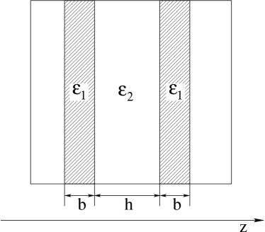
Figure 1: Symmetric triple layer.

$$\begin{split}\epsilon(z)&=\epsilon_{2}+(\epsilon_{1}-\epsilon_{2})\theta(z)+(\epsilon_{2}-\epsilon_{1})\theta(z-b)\\ &+(\epsilon_{1}-\epsilon_{2})\theta(z-b-h)+(\epsilon_{2}-\epsilon_{1})\theta(z-2b-h)\end{split}$$ (9)

where $\theta(z)$ is the Heaviside step function.

The interaction energy per unit area is given by [3, 4]:

$$\begin{split}\mathcal{F}(h,b)&=\\ &\frac{k_{B}T}{4\pi}\int_{0}^{\infty}dp\,p\,\mbox{ln}\left[1-\frac{\Delta^{2}(1-e^{-2bp})^{2}e^{-2hp}}{(1-\Delta^{2}e^{-2bp})^{2}}\right]\end{split}$$ (10)

where

$$\Delta=\frac{\epsilon_{2}-\epsilon_{1}}{\epsilon_{2}+\epsilon_{1}}$$ (11)

One can also consider the pairwise approximation to the general result given by Eq. 10. The major contribution to the integral with respect to $p$ comes from the saddle point $p\approx 0$. Hence we can write, since $\Delta^{2}<1$,

$$\mbox{ln}(1-\Delta^{2}e^{-2hp})\simeq-\Delta^{2}e^{-2hp},$$ (12)

and carry out the integration with respect to $p$ to find [3]

$$\mathcal{F}(h,b)\simeq-\frac{k_{B}T}{16\pi}\left(\frac{\Delta^{2}}{h^{2}}+\frac{\Delta^{2}}{(h+2b)^{2}}+\frac{2\Delta^{2}}{(h+b)^{2}}\right)$$ (13)

In the case of two infinite slabs $b\to\infty$ we have the usual result of Hamaker theory [21]:

$$\mathcal{F}_{H}(h,b\to\infty)=-\frac{k_{B}T\Delta^{2}}{16\pi h^{2}}\equiv-\frac{A}{12\pi h^{2}}$$ (14)

where $A$ is the classical part of the Hamaker constant.

3 A local Monte Carlo algorithm for generating Van der Waals interactions

In the following we describe our simulation method. At zero temperature the Coulomb interaction results from minimizing the energy

$$\mathcal{U}=\frac{1}{2}\int\frac{\mathbf{D}^{2}}{\epsilon(\mathbf{r})}d^{3}\mathbf{r}$$ (15)

where $\epsilon(\mathbf{r})$ is assumed isotropic and $\mathbf{D}$ is the electric displacement constrained by Gauss´ law, $\mathbf{\nabla}\cdot\mathbf{D}=\rho$; $\rho$ is the external charge density. We assume throughout the paper that the dielectric constant of the vacuum is $\epsilon_{0}=1$. This constrained minimization problem for $\mathbf{D}$ can be solved with the help of a Lagrange multiplier $\phi(\mathbf{r})$ by looking for stationary points of the functional $\mathbf{D}$ [22],

$$\mathcal{U}[\mathbf{D}]=\int\left\{\frac{\mathbf{D}^{2}}{2\epsilon(\mathbf{r})}-\phi(\mathbf{r})(\mathbf{\nabla}\cdot\mathbf{D}(\mathbf{r})-\rho(\mathbf{r}))\right\}d^{3}\mathbf{r}$$ (16)

and is given by

$$\mathcal{U}_{0}=\frac{1}{2}\int\epsilon(\mathbf{r})(\mathbf{\nabla}{\phi})^{2}\,d^{3}\mathbf{r}$$ (17)

$\phi$ is the solution of the Poisson equation

$$\mathbf{\nabla}\cdot\mathbf{(}\epsilon(\mathbf{r})\mathbf{\nabla}{\phi})=-\rho$$ (18)

The true interest of the formulation appears in Monte Carlo since one can generate local dynamic systems which sample the partition function

$$\mathcal{Z}=\int\prod_{i=1}^{N}d^{3}\mathbf{r}_{i}\prod_{\mathbf{r}}\mathcal{D}\mathbf{D}(\mathbf{r})\delta(\mathbf{\nabla}\cdot\mathbf{D}-\rho(\mathbf{r}))e^{-\frac{\beta}{2}\int\mathbf{D}^{2}/\epsilon(\mathbf{r})d^{3}\mathbf{r}}$$ (19)

Following [13] we discretize the system placing particles on a simple cubic lattice with vector fields such as ${\mathbf{D}}$ on the links. This formulation is numerically efficient because a local variation in $\rho$ requires only a local update of the field ${\mathbf{D}}$. For problems involving dielectric inhomogeneities (macroparticles with dielectric constant differing from the surroundings) one has to choose an appropriately interpolated value of the dielectric function. The dielectric function is placed also on the link (Ref. [14]) and is given by the harmonic average

$$\frac{2}{\epsilon_{n\mu}}=\frac{1}{\epsilon_{n}}+\frac{1}{\epsilon_{n+\mu}}$$ (20)

where $\{n\mu\}$ is the link which goes from the site $n$ in the $\mu$–direction, $\mu=1,\,2,\,3$. In the absence of charged particles the partition function Eq. 19 becomes

$$\mathcal{Z}=\int\prod_{\mathbf{r}}\mathcal{D}\mathbf{D}(\mathbf{r})\delta(\mathbf{\nabla}\cdot\mathbf{D})e^{-\frac{\beta}{2}\int\mathbf{D}^{2}/\epsilon(\mathbf{r})d^{3}\mathbf{r}}$$ (21)

Introducing an auxiliary field $\phi$ to implement the Gauss’ law constraint and using the identity $2\pi\delta(x)=\int e^{i\phi x}\,d\phi$ the last equation is equivalent to

$$\begin{split}\mathcal{Z}&=C_{1}\int\prod_{\mathbf{r}}d\phi\prod_{\mathbf{r}}\mathcal{D}\mathbf{D}e^{i\int\phi\mathbf{\nabla}\cdot\mathbf{D}d^{3}\mathbf{r}-\frac{\beta}{2}\int\mathbf{D}^{2}/\epsilon(\mathbf{r})d^{3}\mathbf{r}}\\ &=C_{1}\int\prod_{\mathbf{r}}d\phi\prod_{\mathbf{r}}\mathcal{D}\mathbf{D}e^{-i\int\mathbf{D}\mathbf{\nabla}{\phi}d^{3}\mathbf{r}-\frac{\beta}{2}\int\mathbf{D}^{2}/\epsilon(\mathbf{r})d^{3}\mathbf{r}}\\ &=C_{2}\prod_{\mathbf{r}}\epsilon(\mathbf{r})^{3/2}\int\prod_{\mathbf{r}}d\phi e^{-\frac{1}{2\beta}\int\epsilon(\mathbf{r})\,(\mathbf{\nabla}{\phi})^{2}d^{3}\mathbf{r}}\\ &=C_{3}\left[\mbox{det}(-\mathbf{\nabla}\cdot\epsilon(\mathbf{r})\mathbf{\nabla})\right]^{-1/2}\end{split}$$ (22)

where the constants $C_{1}$, $C_{2}$ and $C_{3}$ are of no further interest . Comparing Eq. 22 and Eq. 8 we conclude that our method produces the zero-frequency term of the Lifshitz interaction. One has to note, in spite of the fact that intermediate expressions in deriving Eq. 22 contain complex contributions, the algorithm directly samples the real constrained partition function given by Eq. 19.

4 Numerical validation

We simulate a triple slab system Fig. 1 with two values of dielectric constant of the media: $\epsilon_{1}=2$ and $\epsilon_{1}=78$ using different values of the lattice constant $a$. The dielectric constant of the intermediate region is $\epsilon_{2}=1$ for both cases. The size of the box is $L=15.0$, the width of the slab $b=1.0$.

In order to calculate the free energy we perform a thermodynamic integration [23]. For the reference system (denoted by $I$) the uniform dielectric constant $\epsilon_{2}=1.0$ is assigned.We sample the system with the potential energy $\mathcal{U}$ which depends linearly on the coupling parameter $\lambda$:

$$\begin{split}\mathcal{U}(\lambda)&=(1-\lambda)\mathcal{U}_{I}+\lambda\mathcal{U}_{II}\\ &=(1-\lambda)\int d^{3}\mathbf{r}\frac{\mathbf{D}^{2}}{2\epsilon_{2}}+\lambda\int d^{3}\mathbf{r}\frac{\mathbf{D}^{2}}{2\epsilon(\mathbf{r})}\end{split}$$ (23)

For $\lambda=1$ we recover our system of interest (denoted by $II$). The system with energy $U(\lambda)$ is equivalent to the system with the following dielectric function:

$$\epsilon_{t}(\lambda,\mathbf{r})=\frac{\epsilon(\mathbf{r})\epsilon_{2}}{\epsilon(\mathbf{r})+\lambda(\epsilon_{2}-\epsilon(\mathbf{r}))}$$ (24)

Finally, the free energy difference between systems $II$ and $I$ can be found from the following expression:

$$\mathcal{F}(II)-\mathcal{F}(I)=\int_{0}^{1}d\lambda\left<\frac{\partial\mathcal{U}}{\partial\lambda}\right>_{\lambda}$$ (25)

where $\left<...\right>_{\lambda}$ denotes an ensemble average for a system with energy Eq. 23.

The numerical calculation of a free energy is always demanding. We have approximated the integral in Eq. 25 by a summation over 20 intervals in $\lambda$. The fluctuating field $\mathbf{D}$ is sampled by a worm algorithm [24, 25]. Simulation at each $\lambda$ point involved an equilibration period of $800$ sweeps, where a sweep is 20 worms, followed by a consequent run of another $800$ sweeps configurations. The error bars and average values of free energy have been calculated from $500$ values of free energy. Simulations were performed on an AMD Opteron 2.4GHz processor. Total simulation time for a one measured point was 2 days for $a=1.0$ and 24 days for $a=0.5$.

The free energy calculated in this way gives the full contribution which includes self–energies of individual slabs as well as the interaction energy between slabs. In contrast Eqs. 13 and 10 represent only the interaction part of the excess free energy. In a system with periodic boundary conditions it is difficult to calculate the limit $h\to\infty$ which corresponds to calculating the self–energy part. Therefore we perform an interpolation of our simulation results by the function Eq. 13 and extrapolate them to the region $h\to\infty$ to find the asymptotic value. Further we subtract this contribution from the total free energy Eq. 25. Of course such a procedure leads to small deviations from the analytic curve which can be clearly seen on the corresponding plots.

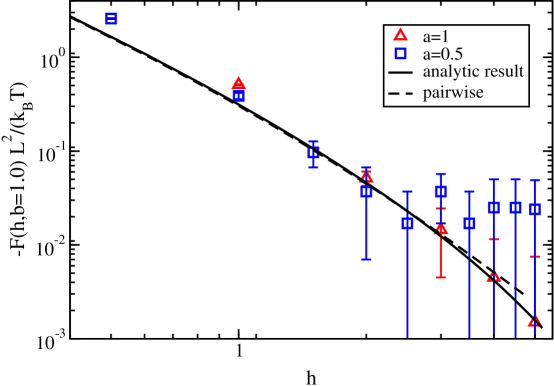
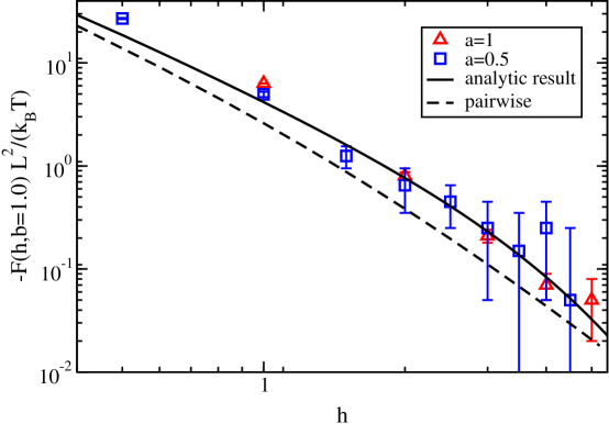
Figure 2: Free energy of the slab at $\epsilon_{1}=2$.

Figure 3: Free energy of the slab at $\epsilon_{1}=78$.

We are interested in observing the free energy of the system as we change the separation between slabs. Our results are shown in Fig. 3 for $\epsilon_{1}=2.0$ and in Fig. 3 for $\epsilon_{1}=78.0$. In both cases, a comparison of results for two different values of the lattice constant $a=0.5;\,1.0$ shows that the errors due to lattice discretization are small. In particular, the data reproduce the analytic result Eq. 10 which differs significantly from the pairwise (Hamaker) curve Eq. 13 for large dielectric contrasts.

5 Conclusion

We have shown that a recent Monte Carlo algorithm for the simulation of electrostatic interactions in heterogeneous dielectric media implicitly generates the zero-frequency part of the Lifshitz interaction including all many-body effects. The interactions make the dominant contribution to the Van der Waals attraction in hydrocarbon-water systems as they are typically found in soft and biological condensed matter [9]. The method is easily applicable to systems with interfaces and spatially varying dielectric constants of arbitrary geometry and allows the inclusion of fixed and free charges.

References

- [1] V.A. Parsegian and B.W Ninham. Temperature-Dependent van der Waals Forces. Biophysical Journal, 10:664, 1970.
- [2] Podgronik R., R.H. French, and Parsegian V.A. Nonadditivity in van der Waals interactions within multilayers. Journal of Chemical Physics, 124:044709, 2006.
- [3] B.W Ninham and V.A. Parsegian. van der Waals Forces across Triple-Layer Films. Journal of Chemical Physics, 52(9):4578, 1970.
- [4] D.S. Dean and R.R. Horgan. Electrostatic fluctuations in soap films. Physical Review E, 65:061603, 2002.
- [5] R.R. Netz. Static van der Waals interaction in electrolytes. European Physical Journal E, 5(189), 2001.
- [6] B.J. Reynwar, G. Illya, V.A. Harmandaris, M.M. Muller, K. Kremer, and M. Deserno. Aggregation and vesiculation of membrane proteins by curvature-mediated interactions. Nature, 447:461–464, 2007.
- [7] B. Roux and T. Simonson. Implicit solvent models. Biophyiscal Chemistry, 78:1–20, 1999.
- [8] H.J. Limbach and C. Holm. Single-Chain Properties of Polyelectrolytes in Poor Solvent. J. Phys. Chem. B., 107:8041–8055, 2003.
- [9] J.N. Israelachvili. Intermolecular and Surface Forces. Academic Press, 1992.
- [10] R. Everaers and M.R. Ejtehadi. Interaction potentials for soft and hard ellipsoids. Physical Review E, 67:041710, 2003.
- [11] C. Schutz and A. Warshel. What are the dielectric ”constants” of proteins and how to validate electrostatic models? PROTEINS-STRUCTURE FUNCTION AND GENETICS, 44:400, 2001.
- [12] J. Mahanty and B.W. Ninham. Dispersion Forces. Academic Press, London, 1976.
- [13] A.C. Maggs and V. Rossetto. Local Simulation Algorithms for Coulomb Interactions. Phys. Rev. Lett., 88:196402, 2002.
- [14] A.C. Maggs. Auxiliary field Monte Carlo for charged particles. Journal of Chemical Physics, 120:3108–3118, 2004.
- [15] A.C. Maggs and R. Everaers. Simulating nanoscale dielectric response. Physical Review Letters, 96:230603, 2006.
- [16] I.E. Dzyaloshinskii, E.M. Lifshitz, and L.P. Pitaevski. The general theory of van der Waals forces. Advances in Physics, 10(38):165, 1961.
- [17] L.D. Landau and E.M. Lifshitz. Electrodynamics of continuous media. Pergamon, 1998.
- [18] J.O. Hirschfelder, C.F. Curtiss, and R.B. Bird. Molecular theory of gases and liquids, chapter 13, page 988. New York, Wiley, 1964.
- [19] D. Bailin and A. Love. Introduction to gauge field theory. IOP Publ., 1993.
- [20] L.D. Landau and E.M. Lifshitz. Statistical Physics (Course of Theoretical Physics, Volume 5). Butterworth-Heinemann, 2000.
- [21] H.C. Hamaker. The London - Van Der Waals attraction between spherical particles. Physica, 4:1058, 1937.
- [22] J. Schwinger, L.L. DeRaad, K.A. Milton, and Wu-yang Tsai. Classical Electrodynamics. Perseus Books, 1998.
- [23] D. Frenkel and B. Smit. Understanding Molecular Simulation. Academic Press, 2002.
- [24] L. Levrel, F. Alet, J. Rottler, and A.C. Maggs. Local Simulation Algorithms for Coulombic Interactions. PRAMANA – journal of physics, 64:1001, 2005.
- [25] F. Alet and E.S. Sorensen. Cluster Monte Carlo algorithm for the quantum rotor model. Physical Review E, 67:015701, 2003.