Monitoring atom-atom entanglement and decoherence
in a solvable tripartite open system in cavity QED

Abstract

We present a fully analytical solution of the dynamics of two strongly-driven atoms resonantly coupled to a dissipative cavity field mode. We show that an initial atom-atom entanglement cannot be increased. In fact, the atomic Hilbert space divides into two subspaces, one of which is decoherence free so that the initial atomic entanglement remains available for applications, even in presence of a low enough atomic decay rate. In the other subspace a measure of entanglement, decoherence, and also purity, are described by a similar functional behavior that can be monitored by joint atomic measurements. Furthermore, we show the possible generation of Schrödinger-cat-like states for the whole system in the transient regime, as well as of entanglement for the cavity field and the atom-atom subsystems conditioned by measurements on the complementary subsystem.

I Introduction

The interaction of a two-level system with a quantized single mode of a harmonic oscillator, named Jaynes-Cummings (JC) model JaynesCummings , is arguably the most fundamental quantum system describing the interaction of matter and light. The JC model has found its natural playground in the field of cavity quantum electrodynamics (CQED), in the microwave ReviewParis ; ReviewGarching and in the optical regime ReviewOptical , as well as in other physical systems, like trapped ions ReviewIons or Circuit ReviewYale and solid-state SSCQED QED. Extensions of the JC model to more atoms and more modes, externally driven or not, have been developed and, presently, we enjoy a vast number of theoretical and experimental developments. Unfortunately, a great part of them are not easy to handle and most of the interesting physics has to be extracted from heavy numerical solutions and calculations, especially when realistic dissipative processes are taking into account.
The advent of quantum information NielsenChuang has been a fresh input in the field of CQED Haroche-Raimond , reshaping concepts and using it for fundamental tests and initial steps in the demanding field of quantum information processing. Here, coherence and the generation of entanglement play an important role, and in particular the manner in which they are affected by the presence of a dissipative environment SchleichBook . In spite of their relevance, most of the attractive quantum models do not enjoy analytical solutions and the few available ones are not as close to realistic conditions as desired.
In this paper, we consider a system composed by two coherently driven two-level atoms trapped inside a cavity and coupled to one of its quantized modes. The experimental implementation seems to be feasible due to the recent advances in deterministic trapping of atoms in optical cavities  trapped-atoms ; Fortier . We show that under full resonance conditions and negligible atomic decays the system dynamics can be solved analytically also in the presence of cavity field dissipation. With the solutions at hand we are able to monitor the purity of the cavity field and atom-atom subsystems, as well as the entanglement and decoherence dynamics of the latter. Atomic entanglement cannot be generated. However, the quantum correlations of suitable entangled states can remain completely protected in a decoherence-free subspace. In case of atomic states outside this subspace, the decays of quantum entanglement, coherence and purity are remarkably described by the same function.
In Sec. II we introduce the master equation of the considered open system, in Sec. III we present the analytical solutions of the system evolution, in Sec. IV we study the dynamics of entanglement in the atom-atom subsystem, in Sec. V we consider the conditional generation of subsystem states, in Sec.VI we present fully numerical results that confirm our analytical developments, and in Sec. VII we conclude with a summary of our results and physical discussions. In the Appendix we discuss the solution of the master equation presented in Sec. II.

II Open System Master Equation

We consider a pair of two-level atoms interacting inside a cavity with a field mode also coupled to the environment (see Fig. 1). A coherent external field of frequency $\omega_{D}$ drives both atoms during the interaction with the cavity mode of frequency $\omega_{f}$ Solano-Agarwal ; PavelOptical . The transition frequency $\omega_{a}$ between excited and ground states, $|e\rangle_{j}$ and $|g\rangle_{j}$ ($j=1,2$), respectively, is the same for the two-level atoms. This system could be experimentally implemented with two-level Rydberg atoms in a microwave cavity Haroche-Raimond or with three-level atoms reduced effectively to two levels interacting with an optical cavity. Relevant advances in cooling and trapping atoms in optical cavities have been recently achieved trapped-atoms ,Fortier . Similar dynamics could be also implemented in trapped ions interacting with a vibrational mode instead of the cavity mode Haroche-Raimond .
The Hamiltonian which describes the whole system unitary dynamics is

$$\hat{\mathcal{H}}(t) = \frac{\hbar\omega_{a}}{2}\sum_{j=1}^{2}\hat{\sigma}^{z}_{j}+\hbar\omega_{f}\hat{a}^{{\dagger}}\hat{a}+\hbar\Omega\sum_{j=1}^{2}\bigg{(}e^{-i\omega_{D}t}\hat{\sigma}_{j}^{{\dagger}}+\,$$ (1)

$$+ e^{i\omega_{D}t}\hat{\sigma}_{j}\bigg{)}+\hbar g\sum_{j=1}^{2}\bigg{(}\hat{\sigma}_{j}^{{\dagger}}\hat{a}+\hat{\sigma}_{j}\hat{a}^{{\dagger}}\bigg{)},$$

where $\Omega$ is the Rabi frequency associated with the coherent driving field amplitude, $g$ the atom-cavity mode coupling constant (taken equal for both atoms), $\hat{a}$ ($\hat{a}^{{\dagger}}$) the field annihilation (creation) operator, $\hat{\sigma}_{j}=|g\rangle_{j}\langle e|$ ($\hat{\sigma}_{j}^{{\dagger}}=|e\rangle_{j}\langle g|$) the atomic lowering (raising) operator, and $\hat{\sigma}^{z}_{j}=|e\rangle_{j}\langle e|-|g\rangle_{j}\langle g|$ the inversion operator.

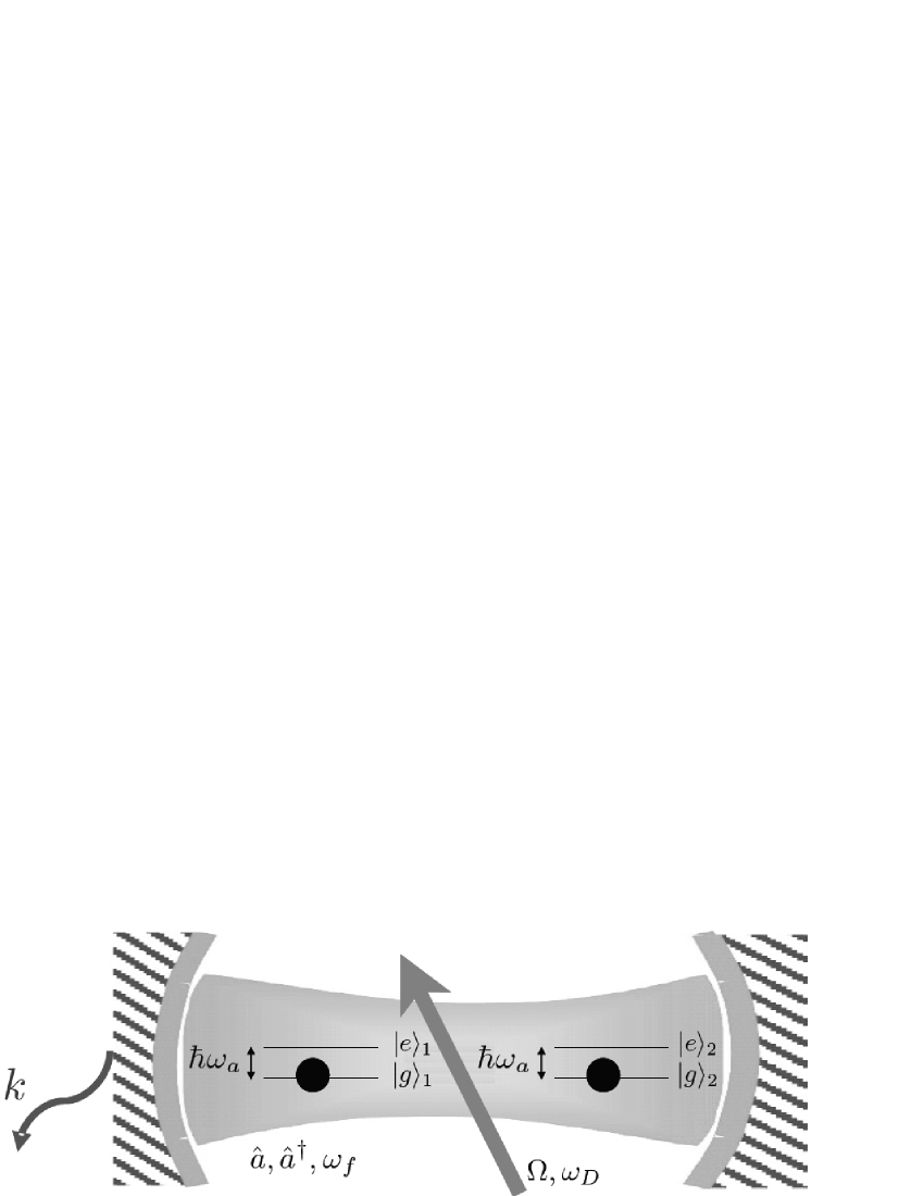
Figure 1: Two driven two-level atoms interacting with a dissipative cavity mode.

In the perspective of possible experimental implementation of our scheme we must include the effects of cavity mode dissipation and the decay of the atomic upper level. Therefore, we must solve the following master equation (ME) for the statistical density operator $\hat{\rho}^{\prime}$ of the whole tripartite system

$$\dot{\hat{\rho}}^{\prime}=-\frac{i}{\hbar}[\hat{\mathcal{H}},\hat{\rho}^{\prime}]+\hat{\mathcal{L}}_{f}\hat{\rho}^{\prime}+\hat{\mathcal{L}}_{a}\hat{\rho}^{\prime}$$ (2)

where

$$\hat{\mathcal{L}}_{f}\hat{\rho}^{\prime} = \frac{k}{2}[2\hat{a}\hat{\rho}^{\prime}\hat{a}^{{\dagger}}-\hat{a}^{{\dagger}}\hat{a}\hat{\rho}^{\prime}-\hat{\rho}^{\prime}\hat{a}^{{\dagger}}\hat{a}]\,$$

$$\hat{\mathcal{L}}_{a}\hat{\rho}^{\prime} = \frac{\gamma}{2}\sum_{j=1}^{2}[2\hat{\sigma}_{j}\hat{\rho}^{\prime}\hat{\sigma}_{j}^{{\dagger}}-\hat{\sigma}_{j}^{{\dagger}}\hat{\sigma}_{j}\hat{\rho}^{\prime}-\hat{\rho}^{\prime}\hat{\sigma}_{j}^{{\dagger}}\hat{\sigma}_{j}],$$ (3)

where $k$ and $\gamma$ are the cavity and atomic decay rates, respectively, and the environment is modeled by a thermal bath at zero temperature.
Changing to the interaction picture the dissipative terms remain unchanged and the ME (2) can be rewritten as

$$\dot{\hat{\rho}}_{I}=-\frac{i}{\hbar}[\hat{\mathcal{H}}_{I},\hat{\rho}_{I}]+\hat{\mathcal{L}}_{f}\hat{\rho}_{I}+\hat{\mathcal{L}}_{a}\hat{\rho}_{I}$$ (4)

where Hamiltonian (1) has been replaced by the time-independent Hamiltonian $\hat{\mathcal{H}}_{I}=\hat{\mathcal{H}}_{0}+\hat{\mathcal{H}}_{1}$ with

$$\hat{\mathcal{H}}_{0} = -\hbar\delta\hat{a}^{{\dagger}}\hat{a}+\hbar\Omega\sum_{j=1}^{2}\left(\hat{\sigma}_{j}^{{\dagger}}+\hat{\sigma}_{j}\right)\,$$

$$\hat{\mathcal{H}}_{1} = \hbar g\sum_{j=1}^{2}\left(\hat{\sigma}_{j}^{{\dagger}}\hat{a}+\hat{\sigma}_{j}\hat{a}^{{\dagger}}\right),$$ (5)

where we introduced the atom-cavity field detuning parameter $\delta=\omega_{a}-\omega_{f}$, and from now on we consider a resonance condition between the atoms and the external field ($\omega_{D}=\omega_{a}$). We remark that Hamiltonian (II) was derived by a standard technique, whereas in the case of less simple systems, e.g. three-level atoms, more refined treatments are necessary to derive a time-independent Hamiltonian such as adiabatic elimination or nonlinear rotations, as e.g. in SDOAL .
The ME (4) can be solved only by numerical techniques, as we discuss in Sec.VI where we present some numerical results for the whole system dynamics. On the other hand, if we consider negligible atomic decay ($\gamma=0$) it is possible to solve Eq.(4) analytically. First of all, we consider the unitary transformation $\hat{\mathcal{U}}(t)=exp\{\frac{i}{\hbar}\hat{\mathcal{H}}_{0}t\}$ and we derive for the density operator $\hat{\rho}(t)=\hat{\mathcal{U}}(t)\hat{\rho}_{I}(t)\hat{\mathcal{U}}^{\dagger}(t)$ the following ME:

$$\dot{\hat{\rho}}=-\frac{i}{\hbar}[\hat{\mathcal{U}}\hat{\mathcal{H}}_{1}\hat{\mathcal{U}}^{\dagger},\hat{\rho}]+\hat{\mathcal{L}}_{f}\hat{\rho}$$ (6)

where the transformed Hamiltonian can be written as

$$\hat{\mathcal{U}}\hat{\mathcal{H}}_{1}\hat{\mathcal{U}}^{\dagger} = \frac{\hbar g}{2}\sum_{j=1}^{2}\big{[}|+\rangle_{j}\langle+|-|-\rangle_{j}\langle-|+e^{2i\Omega t}|+\rangle_{j}\langle-|\,$$ (7)

$$- e^{-2i\Omega t}|-\rangle_{j}\langle+|\big{]}ae^{-i\delta t}+{\rm H.c.}.$$

Here, $\{|+\rangle_{j},|-\rangle_{j}\}$ ($j=1,2$) is a rotated basis connected to the standard basis $\{|e\rangle_{j},|g\rangle_{j}\}$ via $|\pm\rangle_{j}=\frac{|g\rangle_{j}\pm|e\rangle_{j}}{\sqrt{2}}$. In the strong-driving regime for the interaction between the atoms and the external coherent field, $\Omega\gg g$, we can use the rotating-wave approximation (RWA) obtaining the effective Hamiltonian Solano-Agarwal ; PavelOptical

$$\hat{\mathcal{H}}_{\rm eff}(t)=\frac{\hbar g}{2}\sum_{j=1}^{2}(\hat{\sigma}_{j}^{{\dagger}}+\hat{\sigma}_{j})(\hat{a}e^{i\delta t}+\hat{a}^{{\dagger}}e^{-i\delta t}).$$ (8)

Equation (8) outlines the presence of Jaynes-Cummings ($\hat{\sigma}_{j}^{{\dagger}}\hat{a}+\hat{\sigma}_{j}\hat{a}^{{\dagger}}$) as well as anti-Jaynes-Cummings ($\hat{\sigma}_{j}^{{\dagger}}\hat{a}^{{\dagger}}+\hat{\sigma}_{j}\hat{a}$) interaction terms of each coherently driven atom with the cavity mode. We remark that in the framework of trapped ions a similar Hamiltonian can be found but the cavity mode is replaced by the vibrational mode of the ions system KikeIons . In the following we will describe the solution of the effective ME:

$$\dot{\hat{\rho}}=-\frac{i}{\hbar}[\hat{\mathcal{H}}_{\rm eff}(t),\hat{\rho}]+\hat{\mathcal{L}}_{f}\hat{\rho}.$$ (9)

III Exact Solution at resonance for atoms prepared in the ground state

In this section we consider the solution of the ME (9) in the case of exact resonance $\delta=0$, cavity field initially in the vacuum state, and both atoms prepared in the ground state as an example of separable initial state. We leave to future treatments the cases of cavity field prepared in more general states. The exact solution of the ME for any atomic preparation is described in details in the Appendix. It is based on the following decomposition for the density operator $\hat{\rho}(t)$ of the whole system:

$$\hat{\rho}(t)=\sum_{i,j=1}^{4}\langle i|\hat{\rho}(t)|j\rangle|i\rangle\langle j|=\sum_{i,j=1}^{4}\hat{\rho}_{ij}(t)|i\rangle\langle j|$$ (10)

where $\{|i\rangle\}_{i=1}^{4}=\{|++\rangle,|+-\rangle,|-+\rangle,|--\rangle\}$ is the rotated basis of the atomic Hilbert space. Here we report only the final expressions for the field operators $\hat{\rho}_{ij}$ in the present case:

$$\hat{\rho}_{(11,44)}(t) = \frac{1}{4}|\mp\alpha(t)\rangle\langle\mp\alpha(t)|\,$$

$$\hat{\rho}_{(12,13)}(t) = \frac{1}{4}\frac{f_{1}(t)}{e^{-|\alpha(t)|^{2}/2}}|-\alpha(t)\rangle\langle 0|\,$$

$$\hat{\rho}_{14}(t) = \frac{1}{4}\frac{f_{2}(t)}{e^{-2|\alpha(t)|^{2}}}|-\alpha(t)\rangle\langle\alpha(t)|\,$$

$$\hat{\rho}_{(22,23,33)}(t) = \frac{1}{4}|0\rangle\langle 0|\,$$

$$\hat{\rho}_{(24,34)}(t) = \frac{1}{4}\frac{f_{1}(t)}{e^{-|\alpha(t)|^{2}/2}}|0\rangle\langle\alpha(t)|,$$ (11)

where we introduced the time dependent coherent field amplitude

$$\alpha(t)=i\frac{2g}{k}\left(1-e^{-\frac{k}{2}t}\right),$$ (12)

and the function

$$f_{1}(t)=\exp\left\{-\frac{2g^{2}}{k}t+\frac{4g^{2}}{k^{2}}\left(1-e^{-\frac{k}{2}t}\right)\right\}.\\$$ (13)

We recall that $\hat{\rho}_{ji}(t)=\hat{\rho}_{ij}^{\dagger}(t)$. We notice the presence of single atom-cavity field coherences whose evolution is ruled by the function $f_{1}(t)$ SDOAL , as well as full atom-atom-field coherences ruled by $f_{2}(t)=f_{1}^{4}(t)$, that we shall discuss later on. There are also two one-atom coherences, and two diagonal terms, which do not evolve in time, corresponding to a pure state

$$|0\rangle\otimes(|+-\rangle+|-+\rangle)=|0\rangle\otimes(|gg\rangle-|ee\rangle),$$ (14)

where we recognize (up to normalization) a Bell atomic state $|\Phi^{-}\rangle$. The explanation goes as follows. First of all, if we start with atoms prepared in states of the rotated basis used in the decomposition of (10), we obtain much simpler results due to the structure of Hamiltonian (8) on resonance and the obvious uninfluence of dissipation on the cavity vacuum. Actually, either the field states are coherent, $|0\rangle\otimes|\pm\pm\rangle\mapsto|\mp\alpha(t)\rangle\otimes|\pm\pm\rangle$, or there is no evolution at all for the states $|0\rangle\otimes|\pm\mp\rangle$, showing the presence of an invariant subspace for system dynamics. It is the component of the initial state $|0\rangle\otimes|gg\rangle$ in that subspace, (14), which does not evolve. We note that starting from atoms prepared in the other elements of the standard basis we obtain solutions quite analogous to (III), as can be easily verified from the Appendix.
In the transient regime ($kt\ll 1$), the decoherence function can be approximated by $f_{1}(t)\simeq e^{-\frac{|\tilde{\alpha}(t)|^{2}}{2}}$ where $\tilde{\alpha}(t)=igt$, and the whole system is described by a pure Schrödinger-cat-like state

$$|\tilde{\psi}(t)\rangle = \frac{1}{2}\bigg{[}|-\tilde{\alpha}(t)\rangle\otimes|++\rangle+|0\rangle\otimes(|+-\rangle+|-+\rangle)\,$$ (15)

$$+ |\tilde{\alpha}(t)\rangle\otimes|--\rangle\bigg{]}.$$

If we rewrite this result in the standard atomic basis

$$|\tilde{\psi}(t)\rangle=\frac{1}{4}\bigg{[}\big{(}|-\tilde{\alpha}(t)\rangle-2|0\rangle+|\tilde{\alpha}(t)\rangle\big{)}\otimes|ee\rangle\,$$

$$+\big{(}|-\tilde{\alpha}(t)\rangle-|\tilde{\alpha}(t)\rangle\big{)}\otimes(|eg\rangle+|ge\rangle)\,$$

$$+\big{(}|-\tilde{\alpha}(t)\rangle+2|0\rangle+|\tilde{\alpha}(t)\rangle\big{)}\otimes|gg\rangle\bigg{]}$$ (16)

showing the onset of correlations between atomic states and cavity field cat-like states. For the terms related to the field subsystem we recover expressions analogous to those derived in SDM for a strongly driven micromaser system. Unlike the present system, in that case the atoms pump the cavity mode with a Poissonian statistics, interacting for a very short time such that the cavity dissipation is relevant only in the time intervals between atomic injections. Furthermore, the cavity field states are conditioned on atomic measurements.
At steady state ($kt\to\infty$) the density operator is mixed and given by:

$$\hat{\rho}^{SS} = \frac{1}{4}\bigg{[}|-\alpha^{SS}\rangle\langle-\alpha^{SS}|\otimes|++\rangle\langle++|+|\alpha^{SS}\rangle\langle\alpha^{SS}|\,$$

$$\otimes |--\rangle\langle--|+|0\rangle\langle 0|\otimes\bigg{(}|+-\rangle\langle+-|+\,$$

$$+ |+-\rangle\langle-+|+|-+\rangle\langle+-|+|-+\rangle\langle-+|\bigg{)}\bigg{]}\,$$

with $\alpha^{SS}=2i\frac{g}{k}$. Interestingly, the steady state has not a fully diagonal structure, i.e., it is not completely mixed, in agreement with the previous discussion on the time-dependent solution. The change from a pure state to a mixed one and the degree of mixedness can be we evaluated by the purity of the whole system $\mu(t)=Tr[\hat{\rho}^{2}(t)]$:

$$\mu(t)=\frac{1}{8}\left[3+4\frac{f_{1}^{2}(t)}{e^{-|\alpha(t)|^{2}}}+\frac{f_{2}^{2}(t)}{e^{-4|\alpha(t)|^{2}}}\right].$$ (18)

In Fig. 2 we show $\mu(t)$ as a function of the dimensionless time $kt$ for different values of the dimensionless coupling constant $g/k$. We see that the purity decays rather fast in the strong coupling regime $g/k\gtrsim 1$.

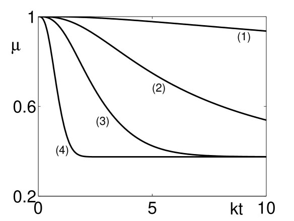
Figure 2: Purity $\mu(t)$ of the whole system density operator vs. dimensionless time $kt$ for dimensionless coupling constant $g/k$: (1) $0.05$, (2) $0.2$, (3) $0.5$, (4) $2$.

III.1 Subsystems dynamics

Now we consider the time evolution of the atomic and cavity field subsystems in the case of both atoms initially prepared in the ground state. The cavity field reduced density operator $\hat{\rho}_{f}(t)=Tr_{a}[\hat{\rho}(t)]$ can be derived by tracing over both atoms:

$$\hat{\rho}_{f}(t) = \frac{1}{4}\bigg{[}|-\alpha(t)\rangle\langle-\alpha(t)|+2|0\rangle\langle 0|+|\alpha(t)\rangle\langle\alpha(t)|\bigg{]}.$$

Hence the cavity field mean photon number is $\langle\hat{N}\rangle=\frac{1}{2}|\alpha(t)|^{2}$ and its steady state value $\langle\hat{N}\rangle_{SS}=2\frac{g^{2}}{k^{2}}$. These results hold for atoms prepared in any state of the standard basis. At any time Eq. (III.1) describes a mixed state, whose purity $\mu_{f}(t)=Tr_{f}[\hat{\rho}_{f}^{2}(t)]$ is:

$$\mu_{f}(t)=\frac{1}{8}\left[3+4e^{-|\alpha(t)|^{2}}+e^{-4|\alpha(t)|^{2}}\right].$$ (20)

In Fig. 3 we show the purity $\mu_{f}(t)$ as a function of dimensionless time $kt$ for different values of the ratio $g/k$, showing a better survival of the purity than for the global state of Fig. 2 except in the strong coupling regime.

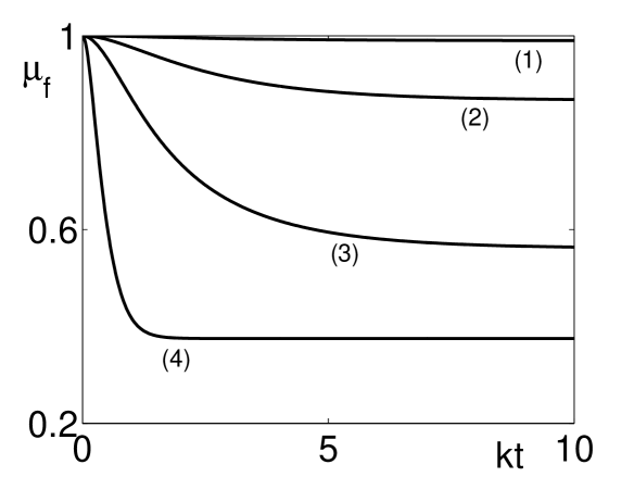
Figure 3: Purity $\mu_{f}(t)$ of the cavity field subsystem vs. dimensionless time $kt$ for dimensionless coupling constant $g/k$: (1) $0.05$, (2) $0.2$, (3) $0.5$, (4) $2$.

The reduced atom-atom density operator $\hat{\rho}_{a}(t)$ can be obtained by tracing over the field variables. In the rotated basis $\{|++\rangle,|+-\rangle,|-+\rangle,|--\rangle\}$, we obtain

$$\rho_{a}^{\pm}(t)=\frac{1}{4}\left(\begin{array}[]{cccc}1&f_{1}(t)&f_{1}(t)&f_{2}(t)\\ f_{1}(t)&1&1&f_{1}(t)\\ f_{1}(t)&1&1&f_{1}(t)\\ f_{2}(t)&f_{1}(t)&f_{1}(t)&1\end{array}\right).$$ (21)

The presence of six time-independent matrix elements is in agreement with the remarks below Eq.(14). The purity $\mu_{a}(t)=Tr_{a}[\hat{\rho}_{a}^{2}(t)]$ of the bi-atomic subsystem is:

$$\mu_{a}(t)=\frac{1}{8}\left[3+4f_{1}^{2}(t)+f_{2}^{2}(t)\right].$$ (22)

Its behavior is quite similar to the one of Fig. 2 for the whole system purity. From Eq. (21) we can derive the single-atom density matrices and evaluate the probability to measure one atom in the excited or ground state

$$P_{{e,g}}(t)=\frac{1}{2}\left[1\mp f_{1}(t)\right].$$ (23)

Quite similar expressions hold for atoms prepared in any state of the standard basis. We see that from measurements of the atomic inversion $I(t)=p_{g}(t)-p_{e}(t)$ we can monitor the one-atom decoherence function $f_{1}(t)$ as in SDOAL . By rewriting the atomic density matrix (21) in the standard basis we evaluate the joint probabilities $P_{lm}(t)=\langle lm|\hat{\rho}_{a}^{(e,g)}(t)|lm\rangle$ with $\{l,m\}=\{e,g\}$. The corresponding correlation functions at a given time $t$ are:

$$C_{ee}(t) = \frac{3-4f_{1}(t)+f_{2}(t)}{2[1-f_{1}(t)]^{2}}\,$$

$$C_{eg}(t) = C_{ge}(t)=\frac{1-f_{2}(t)}{2[1-f_{1}^{2}(t)]}\,$$

$$C_{gg}(t) = \frac{3+4f_{1}(t)+f_{2}(t)}{2[1+f_{1}(t)]^{2}}$$ (24)

In Figs. 4(a-c) we show the correlation functions $C_{lm}(t)$ versus dimensionless time $kt$ and coupling constant $\frac{g}{k}$.

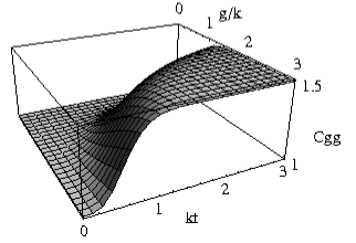
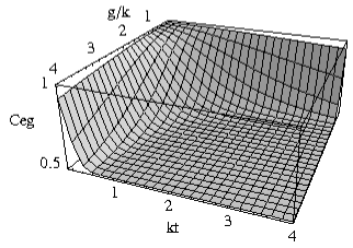
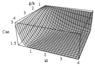
a) b) c)

Figure 4: Correlation functions (a) $C_{gg}$, (b) $C_{eg}$, (c) $C_{ee}$ vs. dimensionless time $kt$ and coupling constant $g/k$, showing atomic bunching and anti-bunching.

At steady-state we see that $C_{gg}(t),C_{ee}(t)\mapsto 3/2$, that is positive atom-atom correlation or bunching, whereas $C_{eg}(t)\mapsto 1/2$, indicating negative correlation or anti-bunching. These results generalize those in SDM , which can be derived from Eqs.(III.1) in the limit of negligible dissipation $kt\ll 1$. We notice that from the joint atomic probability $P_{eg}(t)=P_{ge}(t)=\frac{1}{8}[1-f_{2}(t)]$ one can monitor the two-atom decoherence described by $f_{2}(t)$.

IV Dynamics of entanglement and decoherence of the atomic subsystem

In Sec. III we discussed the solution of the ME (9) for both atoms prepared in the ground state as an example of separable state. In order to describe also initially entangled atoms now we consider the general solution derived in the Appendix for atoms prepared in a superposition of Bell states $|\psi_{a}(0)\rangle=\sum_{i=1}^{4}c_{i}|\nu_{i}\rangle$, where the coefficients $c_{i}$ are normalized as $\sum_{i=1}^{4}|c_{i}|^{2}=1$, and $\{|\nu_{i}\rangle\}_{i=1,..,4}=\{|\Phi^{+}\rangle,|\Phi^{-}\rangle,|\Psi^{+}\rangle,|\Psi^{-}\rangle\}$ is the Bell basis where $|\Phi^{\pm}\rangle=\frac{|ee\rangle\pm|gg\rangle}{\sqrt{2}}$ and $|\Psi^{\pm}\rangle=\frac{|eg\rangle\pm|ge\rangle}{\sqrt{2}}$. Tracing over the atomic variables the solution for the whole density operator (Eqs. (10) and (A)) we derive the cavity field density operator generalizing Eq. (III.1):

$$\hat{\rho}_{f}(t) =\frac{1}{2}\bigg{[}|c_{1}+c_{3}|^{2}|-\alpha(t)\rangle\langle-\alpha(t)|+\,$$

$$+2(|c_{2}|^{2}+|c_{4}|^{2})|0\rangle\langle 0|+|c_{1}-c_{3}|^{2}|\alpha(t)\rangle\langle\alpha(t)|\bigg{]}.$$

For the mean photon number we obtain $\langle\hat{N}\rangle(t)=(|c_{1}|^{2}+|c_{3}|^{2})|\alpha(t)|^{2}$ that is independent of the coefficients of states $|\Phi^{-}\rangle$ and $|\Psi^{-}\rangle$. On the other hand, tracing over the field variables we obtain the atomic density matrix. We report the solution in the so called magic basis Magic that can be obtained from the Bell basis simply multiplying $|\nu_{2}\rangle$ and $|\nu_{3}\rangle$ by the imaginary unit:

$$\rho_{a}^{mB}=\left(\begin{array}[]{cccc}\frac{[1+f_{2}]|c_{1}|^{2}+[1-f_{2}]|c_{3}|^{2}}{2}&-if_{1}c_{1}c_{2}^{*}&-i\frac{[1+f_{2}]c_{1}c_{3}^{*}+[1-f_{2}]c_{1}^{*}c_{3}}{2}&f_{1}c_{1}c_{4}^{*}\\ if_{1}c_{1}^{*}c_{2}&|c_{2}|^{2}&f_{1}c_{2}c_{3}^{*}&ic_{2}c_{4}^{*}\\ i\frac{[1+f_{2}]c_{1}^{*}c_{3}+[1-f_{2}]c_{1}c_{3}^{*}}{2}&f_{1}c_{2}^{*}c_{3}&\frac{[1-f_{2}]|c_{1}|^{2}+[1+f_{2}]|c_{3}|^{2}}{2}&if_{1}c_{3}c_{4}^{*}\\ f_{1}c_{1}^{*}c_{4}&-ic_{2}^{*}c_{4}&-if_{1}c_{3}^{*}c_{4}&|c_{4}|^{2}\end{array}\right),\,$$ (30)

where we omitted the time dependence for brevity. To evaluate the entanglement properties of the atomic subsystem we consider the entanglement of formation $\epsilon_{F}(t)$ EOF defined as

$$\epsilon_{F}(t) = -\frac{1-\sqrt{1-C^{2}(t)}}{2}\log_{2}\frac{1-\sqrt{1-C^{2}(t)}}{2}+\,$$ (32)

$$- \frac{1+\sqrt{1-C^{2}(t)}}{2}\log_{2}\frac{1+\sqrt{1-C^{2}(t)}}{2},$$

where $C(t)$ is the concurrence that can be evaluated as $C(t)=max\{0,\Lambda_{4}(t)-\Lambda_{3}(t)-\Lambda_{2}(t)-\Lambda_{1}(t)\}$ ($\Lambda_{i}$ are the square roots of the eigenvalues of the non hermitian matrix $\rho_{a}^{mB}(t)(\rho_{a}^{mB}(t))^{*}$ taken in decreasing order). From Eq. (30) we can derive the probabilities for joint atomic measurements in the standard basis

$$P_{ee,gg}(t) = \frac{1}{4}\big{[}|c_{1}|^{2}(1+f_{2}(t))+2|c_{2}|^{2}\,$$

$$+ |c_{3}|^{2}(1-f_{2}(t))\pm 4f_{1}(t)Re(c_{1}c_{2}^{*})\big{]}\,$$

$$P_{eg,ge}(t) = -\frac{1}{4}\big{[}|c_{1}|^{2}(1-f_{2}(t))+2|c_{4}|^{2}\,$$ (33)

$$+ |c_{3}|^{2}(1+f_{2}(t))\pm 4f_{1}(t)Re(c_{3}c_{4}^{*})\big{]}.$$

Also, we can derive the density matrix corresponding to a single atom and obtain the atomic probabilities generalizing Eq. (23):

$$P_{e,g}(t)=\frac{1}{2}\left[1\pm 2f_{1}(t)Re(c_{1}^{*}c_{2}+c_{3}^{*}c_{4})\right].$$ (34)

First we consider the case of a superposition of Bell states $|\Phi^{\pm}\rangle$ (i.e., $c_{1}=a,c_{2}=be^{i\theta},c_{3}=c_{4}=0$ with $a,b$ real numbers). The initial atomic state $|gg\rangle$ ($|ee\rangle$) can be obtained if $a=b=\frac{1}{\sqrt{2}}$ and $\theta=\pi$ ( $\theta=0$). We find that the concurrence $C(t)$ vanishes for any time and every value of $g/k$, so that it is not possible to entangle the atoms. In the case of atoms prepared in a partially entangled state we find that the entanglement of formation can only decrease during the system evolution as shown for example in Fig. 5(a) in the case $a=b=\frac{1}{\sqrt{2}}$ and $\theta=\pi/4$. We also see that the progressive loss of entanglement is faster for large values of the parameter $g/k$. For atoms prepared in the maximally entangled state $|\Phi^{+}\rangle$ (i.e., $\theta=0,a=1,b=0$) we derive that the concurrence simply reduces to $f_{2}(t)$ that also describes the whole system decoherence. This important point will be discussed later. In Fig. 5(b) we show the entanglement of formation as a function of dimensionless time $kt$. For atoms prepared in the maximally entangled state $|\Phi^{-}\rangle$ (i.e., $\theta=0,a=0,b=1$) the concurrence is always maximum ($C(t)=1$). In fact, we can see from Eq.(30) that the atomic density matrix is always the one of the initial state, as expected because $|\Phi^{-}\rangle$ is a linear combination of the invariant states $|+-\rangle$ and $|-+\rangle$.

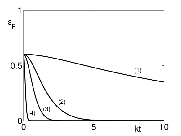
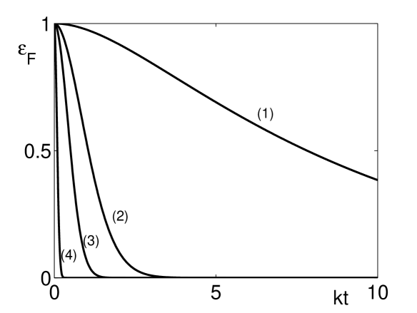
a) b)

Figure 5: Entanglement of formation $\epsilon_{F}(t)$ as a function of $kt$ and for different values of $g/k$: 0.1 (1), 0.5 (2), 1 (3), 5 (4). (a) atoms prepared in a partially entangled state $\frac{|\Phi^{+}\rangle+e^{i\pi/4}|\Phi^{-}\rangle}{\sqrt{2}}$, (b) atoms prepared in the Bell states $|\Phi^{+}\rangle$.

Starting from a superposition of Bell states $|\Psi^{\pm}\rangle$ (i.e., $c_{3}=a,c_{4}=be^{i\theta},c_{1}=c_{2}=0$) we obtain analogous results. In particular entanglement cannot be generated for atoms prepared in states $|eg\rangle$ and $|ge\rangle$, for the state $|\Psi^{+}\rangle$ the concurrence is given by $f_{2}(t)$, and the entanglement of state $|\Psi^{-}\rangle$ is preserved during system evolution. We find analogous results also for the concurrence of atoms prepared in a superposition of $|\Phi^{-}\rangle$ and $|\Psi^{+}\rangle$ (i.e., $c_{2}=a,c_{3}=be^{i\theta},c_{1}=c_{4}=0$) or in a superposition of $|\Phi^{+}\rangle$ and $|\Psi^{-}\rangle$ (i.e., $c_{1}=a,c_{4}=be^{i\theta},c_{2}=c_{3}=0$).
Let us summarize and discuss the main results in the case of atoms prepared in entangled states. If we consider a superposition of states $|\Phi^{-}\rangle$ and $|\Psi^{-}\rangle$ (i.e., $c_{2}=a,c_{4}=be^{i\theta},c_{1}=c_{3}=0$) we find that the atomic density matrix of Eq.(30) does not evolve. Actually, the atomic subspace spanned by $|\Phi^{-}\rangle$ and $|\Psi^{-}\rangle$ coincides with the time-invariant subspace spanned by $|+-\rangle$ and $|-+\rangle$, so that it remains protected from dissipation during the system evolution. It provides an example of Decoherence Free Subspace (DFS)DFS . Atomic entanglement injected in the system can thus remain available for long storage times for applications in quantum information processing Minns .
If we consider a superposition of states $|\Phi^{+}\rangle$ and $|\Psi^{+}\rangle$ (i.e., $c_{1}=a,c_{3}=be^{i\theta},c_{2}=c_{4}=0$) the concurrence is given by:

$$C(t)=\sqrt{a^{4}+b^{4}-2a^{2}b^{2}\cos(2\theta)}f_{2}(t)$$ (35)

and we find the remarkable result that the initial entanglement is progressively reduced by the decoherence function $f_{2}(t)$. Note that $C(t)=f_{2}(t)$ for states $|\Phi^{+}\rangle$, $|\Psi^{+}\rangle$, and any superposition as $a|\Phi^{+}\rangle\pm ib|\Psi^{+}\rangle$. To understand this point let us consider the specific example of the initial state $|0\rangle\otimes|\Phi^{+}\rangle$. The evolved density operator of the whole system is

$$\hat{\rho}(t)=\frac{1}{2}\big{\{}|-\alpha(t)\rangle\langle-\alpha(t)|\otimes|++\rangle\langle++|+\,$$

$$|\alpha(t)\rangle\langle\alpha(t)|\otimes|--\rangle\langle--|+\,$$

$$\frac{f_{2}(t)}{e^{-2|\alpha(t)|^{2}}}\big{[}|-\alpha(t)\rangle\langle\alpha(t)|\otimes\,$$

$$|++\rangle\langle--|+|\alpha(t)\rangle\langle-\alpha(t)|\otimes|--\rangle\langle++|\big{]}\big{\}}.\,$$

In the limit, $kt\ll 1$, of short time and/or negligible dissipation, where $f_{2}(t)\simeq e^{-2|\tilde{\alpha}(t)|^{2}}$ with $\tilde{\alpha}(t)=igt$, the system evolves into a pure cat-like state where the atoms are correlated with coherent states

$$|0\rangle\otimes\frac{|++\rangle+|--\rangle}{\sqrt{2}}\mapsto\frac{|-\tilde{\alpha}\rangle\otimes|++\rangle+|\tilde{\alpha}\rangle\otimes|--\rangle}{\sqrt{2}}.$$ (37)

For longer times/larger dissipation, the system coherence decays as described by the function $f_{2}(t)$. Let us now consider the atomic dynamics disregarding the field subsystem. The reduced atomic density operator is

$$\hat{\rho}_{a}(t)=\frac{1}{2}\big{[}|++\rangle\langle++|+|--\rangle\langle--|\,$$

$$+f_{2}(t)\big{(}|++\rangle\langle--|+|--\rangle\langle++|\big{)}\big{]}.$$ (38)

Hence, as the quantum coherence reduces, simultaneously the atoms lose their inseparability, and the state becomes maximally mixed (in the relevant subspace). In fact, the atomic purity is given by $\mu_{a}(t)=\frac{1+f_{2}^{2}(t)}{2}$. Hence the time evolution of decoherence, concurrence, and purity is described by the function $f_{2}(t)$, which can be monitored via a measurement of joint atomic probabilities (see Eq. (IV))

$$P_{ee}(t) = P_{gg}(t)=\frac{1}{4}\left[1+f_{2}(t)\right]\,$$

$$P_{eg}(t) = P_{ge}(t)=\frac{1}{4}\left[1-f_{2}(t)\right].$$ (39)

The probability $P_{ee}(t)$ is shown in Fig. 6 as a function of $kt$ for different values of the ratio $g/k$. For $kt\ll 1$, when the whole system is in the cat-like state (37), $f_{2}(t)$ quadratically decreases as $\exp{(-2g^{2}t^{2})}$, independent of the dissipative rate $k$. The subsequent behavior is approximately an exponential decay whose start and rate depend on the atom-cavity field coupling. For $g/k\gtrsim 0.5$, that is also below the strong coupling regime, we can introduce a decoherence and disentanglement rate

$$\gamma_{D}\simeq k|\alpha^{SS}|=2g,$$ (40)

that is again independent of (and faster than) $k$. A physical interpretation of this result is that the more coupled the two atoms are to the dissipative cavity mode, the more effective becomes the decay of both the environment-induced decoherence and the initial entanglement. For $g/k\ll 1$, that is in a weak coupling regime, the exponential decay of coherence and concurrence starts later and its rate, $\gamma_{D}\simeq 8g^{2}/k$, is slower than the dissipative rate $k$.

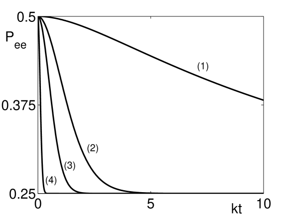
Figure 6: Atoms prepared in the Bell state $|\Phi^{+}\rangle$: joint atomic probability $P_{ee}(t)$ vs. $kt$ for different values of $g/k$: 0.1 (1), 0.5 (2), 1 (3), 5 (4).

We have shown that under full resonance conditions it is not possible to generate or increase the initial atomic entanglement. This can be explained looking at the initial requirements that allow us to write Eq.(48). In particular, the strong driving condition $\Omega\gg g$, the resonance condition $\delta=0$ and the choice of negligible atomic decays $\gamma=0$ are necessary to obtain an independent set of equations for the operators $\hat{\rho}_{ij}$ and to exactly solve the system dynamics. In section VI we will show that removing the strong driving condition it is possible to slightly entangle the atoms. On the other hand, it can be shown CL that with off-resonant atoms-cavity field interaction it is possible to generate maximally entangled atomic states also under strong driving conditions. Also we recall that, in the resonant case and without driving field, two atoms prepared in a separable state can partially entangle by coupling to a thermal cavity field Kim .

V Conditional generation of states

In this section we seek information about the states of one of the two subsystems conditioned by a projective measurement on the other one.
If the system is implemented in the optical domain and the cavity field is accessible to measurements, a null measurement by a on/off detector implies the generation of a maximally entangled atomic Bell state PavelOptical . In the case of atoms prepared in state $|gg\rangle$ (or $|ee\rangle$), the atomic conditioned state will be the Bell state $|\Phi^{-}\rangle$ (see (14)). Analogously, for initial atomic state $|eg\rangle$ or $|ge\rangle$ the atomic conditioned state will be $|\Psi^{-}\rangle$.
Now we consider the evolution of the field subsystem conditioned by a projective atomic measurement on the bare basis $\{|ee\rangle,|eg\rangle,|ge\rangle,|gg\rangle\}$. Starting e.g. from the initial state $|0\rangle\otimes|gg\rangle$, the cavity field will be in the conditioned states at a given time $t$ (omitted for brevity in this section):

$$\hat{\rho}_{f,(ee,gg)} = \frac{1}{2(3+f_{2}\mp 4f_{1})}\bigg{[}|-\alpha\rangle\langle-\alpha|+|\alpha\rangle\langle\alpha|+\,$$

$$+ 4|0\rangle\langle 0|+f_{2}e^{2|\alpha|^{2}}\bigg{(}|\alpha\rangle\langle-\alpha|+|-\alpha\rangle\langle\alpha|\bigg{)}\,$$

$$\mp 2f_{1}e^{\frac{|\alpha|^{2}}{2}}\bigg{(}|0\rangle\langle-\alpha|+|0\rangle\langle\alpha|+\,$$

$$+ |-\alpha\rangle\langle 0|+|\alpha\rangle\langle 0|\bigg{)}\bigg{]}\,$$

$$\hat{\rho}_{f,(eg,ge)} = \frac{1}{2(1-f_{2})}\bigg{[}|-\alpha\rangle\langle-\alpha|+|\alpha\rangle\langle\alpha|\,$$ (41)

$$- f_{2}e^{2|\alpha|^{2}}\bigg{(}|\alpha\rangle\langle-\alpha|+|-\alpha\rangle\langle\alpha|\bigg{)}\bigg{]}.$$

Note that in the limit $kt\ll 1$ the conditioned field state is a Schrödinger-cat-like state

$$|\psi\rangle_{f,(ee,gg)} = \frac{|-\tilde{\alpha}\rangle\mp 2|0\rangle+|\tilde{\alpha}\rangle}{\sqrt{2(e^{-2|\tilde{\alpha}|^{2}}\mp 4e^{-|\tilde{\alpha}|^{2}/2}+3)}}\,$$

$$|\psi\rangle_{f,(eg,ge)} = \frac{|-\tilde{\alpha}\rangle-|\tilde{\alpha}\rangle}{\sqrt{2(1-e^{-2|\tilde{\alpha}|^{2}})}}$$ (42)

where $\tilde{\alpha}(t)=igt$.
The Wigner functions representing the states (V) in phase space at a given time, are:

$$W_{f,(ee,gg)}(\beta) = \frac{2e^{-2|\beta|^{2}}}{\pi(3+f_{2}\mp 4f_{1})}\bigg{[}2+\,$$

$$+ e^{-2|\alpha|^{2}}\cosh(4|\alpha|Im\beta)\,$$

$$+ f_{2}e^{2|\alpha|^{2}}\cos(4|\alpha|Re\beta)\,$$

$$\mp 4f_{1}\cosh(2|\alpha|Im\beta)\cos(2|\alpha|Re\beta)\bigg{]}\,$$

$$W_{f,(eg,ge)}(\beta) = \frac{2e^{-2|\beta|^{2}}}{\pi(1-f_{2})}\bigg{[}e^{-2|\alpha|^{2}}\cosh(4|\alpha|Im\beta)\,$$ (43)

$$- f_{2}e^{2|\alpha|^{2}}\cos(4|\alpha|Re\beta)\bigg{]}.$$

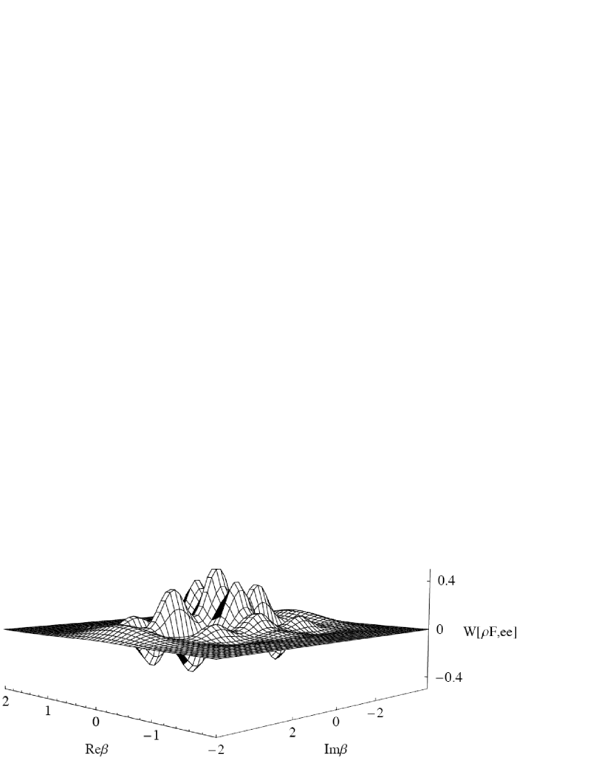
a)
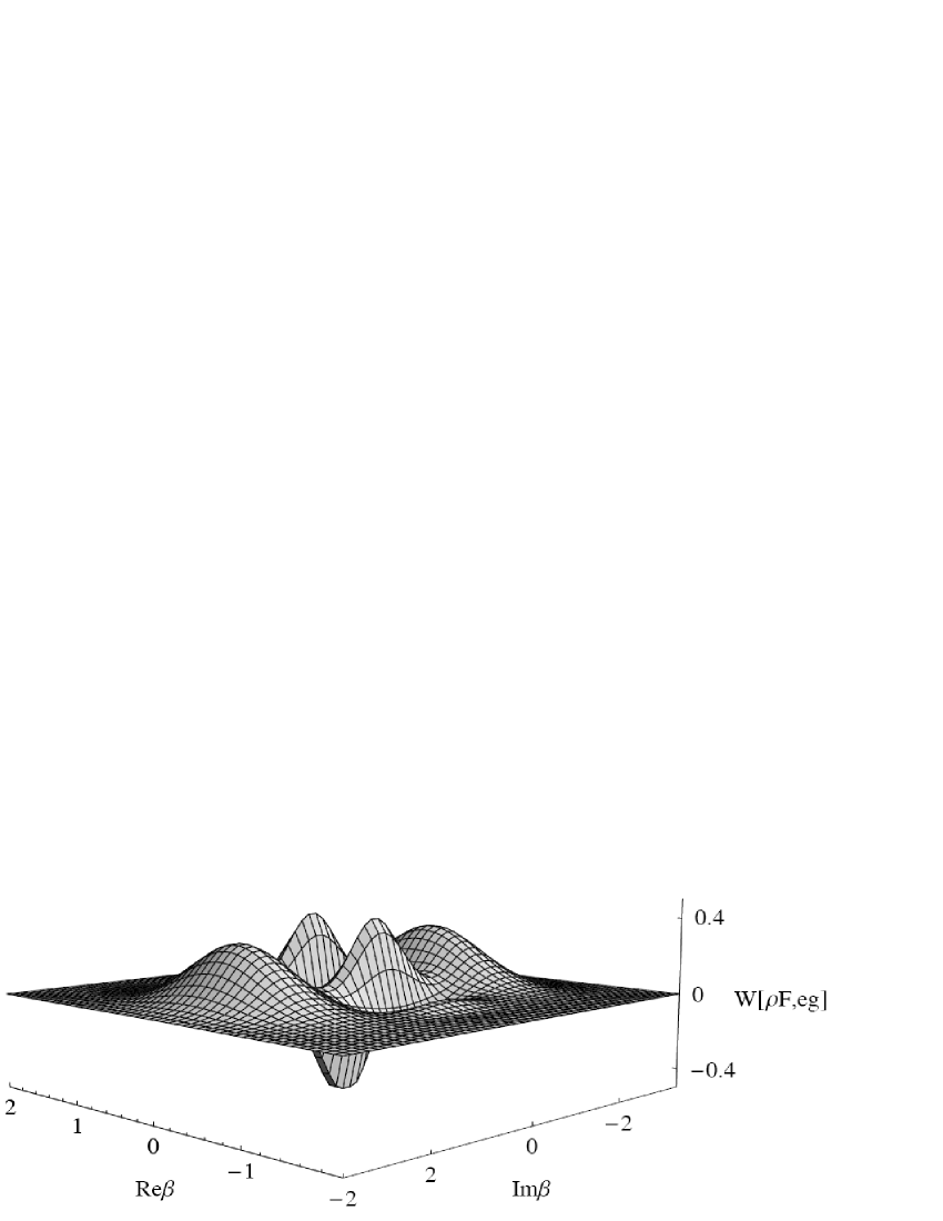
b)

Figure 7: Wigner function of the cavity field $W[\hat{\rho}_{f,(ee)}]$ (a) and $W[\hat{\rho}_{f,(eg)}]$ (b), for $kt=0.05$, and for $\frac{g}{k}=80$ (a) and $\frac{g}{k}=40$ (b).

In Fig. 7 we illustrate two of the Wigner functions (V) in the transient $kt\ll 1$ and in the strong coupling regime $g\gg k$. At steady state the Wigner functions are positive, corresponding to the states:

$$\hat{\rho}^{SS}_{F,(ee,gg)} = \frac{1}{6}\left[|-\alpha^{SS}\rangle\langle-\alpha^{SS}|+|\alpha^{SS}\rangle\langle\alpha^{SS}|+4|0\rangle\langle 0|\right]\,$$

$$\hat{\rho}^{SS}_{F,(eg,ge)} = \frac{1}{2}\left[|-\alpha^{SS}\rangle\langle-\alpha^{SS}|+|\alpha^{SS}\rangle\langle\alpha^{SS}|\right]$$ (44)

where $\alpha^{SS}=i\frac{2g}{k}$.

VI Numerical results

To confirm our theoretical analysis as well as to investigate system dynamics without the strong driving condition and including the effect of atomic decay, where analytical results are not available, we numerically solve, by Monte Carlo Wave Function (MCWF) method MCWF , the ME (4) in the resonant case $\delta=0$, that we rewrite in the Lindblad form:

$$\dot{\hat{\rho}}_{I} = -\frac{i}{\hbar}(\hat{\mathcal{H}}_{e}\hat{\rho}_{I}-\hat{\rho}_{I}\hat{\mathcal{H}}_{e}^{\dagger})+\sum_{i=1}^{3}\hat{C}_{i}\hat{\rho}_{I}\hat{C}_{i}^{\dagger}$$ (45)

where the non-Hermitian effective Hamiltonian $\hat{\mathcal{H}}_{e}$ is given by

$$\hat{\mathcal{H}}_{e}=\frac{\hat{\mathcal{H}}_{I}}{g}-\frac{i\hbar}{2}\sum_{i=1}^{3}\hat{C}_{i}^{\dagger}\hat{C}_{i},$$ (46)

the Hamiltonian $\hat{\mathcal{H}}_{I}$ is that of Eq.(II) for $\delta=0$ , and the collapse operators are $\hat{C}_{1,2}=\sqrt{\tilde{\gamma}}\hat{\sigma}_{1,2}$, $\hat{C}_{3}=\sqrt{\tilde{k}}\hat{a}$. We have introduced the scaled time $\tilde{t}=gt$ so that the relevant dimensionless system parameters are:

$$\tilde{\Omega}=\frac{\Omega}{g}\hskip 14.22636pt\tilde{k}=\frac{k}{g}\hskip 14.22636pt\tilde{\gamma}=\frac{\gamma}{g}.$$ (47)

The system dynamics can be simulated by a suitable number $N_{tr}$ of trajectories, i.e. stochastic evolutions of the whole system wave function $|\psi_{j}(\tilde{t})\rangle$ ($j=1,2,...N_{tr}$). Therefore, the statistical operator of the whole system can be approximated by averaging over the $N_{tr}$ trajectories, i.e., $\hat{\rho}_{I}(\tilde{t})\cong\frac{1}{N_{tr}}\sum_{i=j}^{N_{tr}}|\psi_{j}(\tilde{t})\rangle\langle\psi_{j}(\tilde{t})|$.
First we consider negligible atomic decay $\tilde{\gamma}=0$ to confirm the analytical solutions and to evaluate the effect of the driving parameter $\tilde{\Omega}$. For numerical convenience we consider the case $\tilde{k}=1$ so that the steady state mean photon number assumes small enough values. We consider the atoms prepared in the maximally entangled states $|\Phi^{\pm}\rangle$. We recall that for the state $|\Phi^{+}\rangle$ the theoretical mean photon number is $\langle\hat{N}(\tilde{t})\rangle=|\alpha(\tilde{t})|^{2}$, the atomic populations $P_{e,g}(\tilde{t})=0.5$, the atomic purity $\mu_{a}(\tilde{t})=\frac{1+f_{2}^{2}(\tilde{t})}{2}$, and the entanglement of formation $\epsilon_{F}(t)$ is given by (32) where the concurrence $C(t)$ coincides with $f_{2}(t)$.

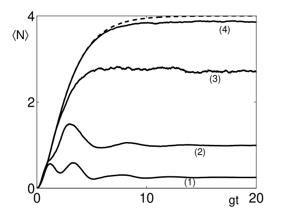
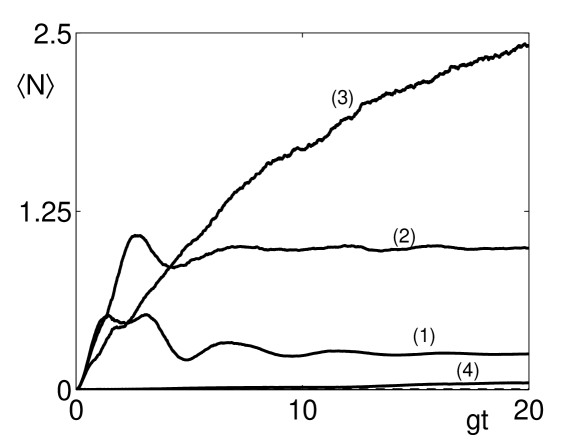
a) b)
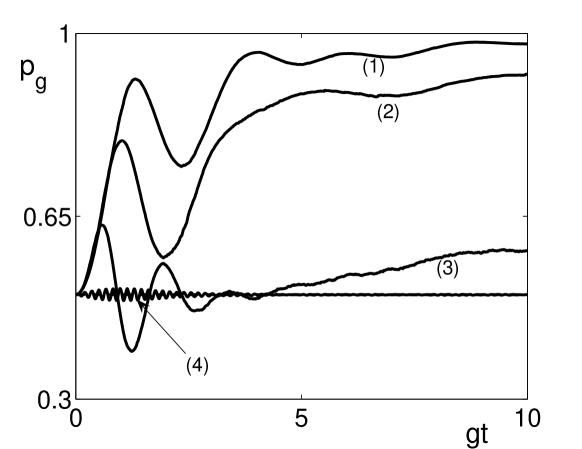
c) d)

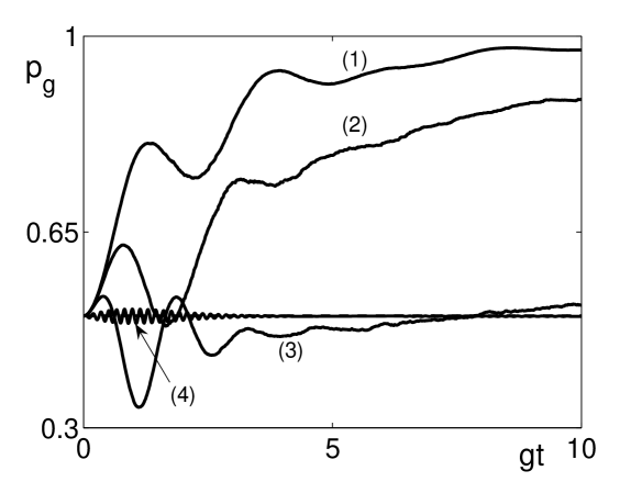
Figure 8: Effect of driving parameter $\tilde{\Omega}$ for negligible atomic decay $\tilde{\gamma}=0$, $\tilde{k}=1$, atoms prepared in the Bell state $|\Phi^{+}\rangle$ ((a),(b)) and $|\Phi^{-}\rangle$ ((c),(d)), for values of $\tilde{\Omega}$: $0.5$ (1), $1$ (2), $2$ (3), $20$ (4). The theoretical functions are the dashed lines. We show in (a),(c) the mean photon number $\langle\hat{N}(\tilde{t})\rangle$, and in (b),(d) the atomic probability $p_{g}(\tilde{t})$ . The number of trajectories is $N_{tr}=500$.

In Fig. 8 we show e.g. the mean photon number and the atomic probability $p_{g}(t)$. In the strong driving limit, $\tilde{\Omega}=20$, we find an excellent agreement with the predicted theoretical behavior. We note that we simulated the system dynamics without the RWA approximation so that $p_{g}(\tilde{t})$ exhibits oscillations due to the driving field. We remark that the entanglement of formation in the case of state $|\Phi^{+}\rangle$ evolves almost independently of parameter $\tilde{\Omega}$ and becomes negligible after times $gt\approx 2$. In the case of state $|\Phi^{-}\rangle$ $\epsilon_{F}(t)$ decays in a similar way for small values of $\tilde{\Omega}$, but it remains close to 1 for large enough values of the driving parameter as predicted in our analysis.
Finally, we consider the effect of the atomic decay. For example, we consider the atoms prepared in the Bell state $|\Phi^{-}\rangle$ in the strong driving limit and for the cavity field decay rate $\tilde{k}=1$. In Fig. 9 we show the mean photon number and the entanglement of formation. We see that for $\tilde{\gamma}$ up to $10^{-3}$ the effect of atomic decays is negligible and the results of our treatment still apply. For larger decay rates the atomic dynamics becomes no more restricted within the decoherence free subspace.

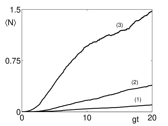
a) b)

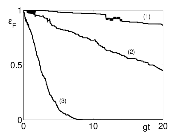
Figure 9: Effect of atomic decay $\tilde{\gamma}$ in the strong driving condition $\tilde{\Omega}=20$, atoms prepared in the Bell state $|\Phi^{-}\rangle$ and $\tilde{k}=1$: $\tilde{\gamma}=0.001$(1), $0.01$ (2), $0.1$ (3). (a) Mean photon number $\langle\hat{N}(\tilde{t})\rangle$, (b) Entanglement of formation $\epsilon_{F}(\tilde{t})$. The number of trajectories is $N_{tr}=500$.

VII Conclusions

We have described the dynamics of a system where a pair of two-level atoms, strongly driven by an external coherent field, are resonantly coupled to a cavity field mode that is in contact with an environment. There are different available or forthcoming routes to the implementation of our model. In the microwave regime of cavity QED pairs of atoms excited to Rydberg levels cross a high-Q superconductive cavity with negligible spontaneous emission during the interaction Haroche-Raimond . Difficulties may arise due to the (ideal) requirements on atomic simultaneous injection, equal velocity, and equal coupling rate to the cavity mode. In the optical regime the application of cooling and trapping techniques in cavity QED trapped-atoms allows the deterministic loading of single atoms in a high-finesse cavity, with accurate position control and trapping times of many seconds Fortier . In this regime laser-assisted three-level atoms can behave as effective two-level atoms with negligible spontaneous emission SDOAL . On the other hand, trapped atomic ions can remain in an optical cavity for an indefinite time in a fixed position, where they can couple to a single mode without coupling rate fluctuations ioncavity . These systems are quite promising to our purposes and could become almost ideal in case of achievement of the strong coupling regime.
Under full resonance conditions and starting from the vacuum state of the cavity field, and for negligible atomic decays and thermal fluctuations, we solved exactly the system dynamics for any initial preparation of the atom pair, thus deriving a number of analytical results on the whole system as well as the different subsystems. These results are confirmed and extended by numerical simulations, e.g. including also atomic decays and investigating regimes under weaker driving conditions.
Here we discuss some results mainly concerning the bi-atomic subsystem. First of all we find that if atoms are prepared in a separable state, no atom-atom entanglement can be generated, in agreement with previous results that showed the classical nature of atom-atom correlations under purely unitary dynamics IJQI . If atoms are initially quantum correlated, their dynamics can be quite different as it can be appreciated in the Bell basis.
If the initial state is any linear combination of the states $|\Phi^{-}\rangle$ and $|\Psi^{-}\rangle$, it does not evolve in time. The atomic subspace is free from cavity dissipation and decoherence, hence the initial entanglement can be preserved for storage times useful for quantum computation/communication purposes Minns .
If the atoms are prepared in any superposition of the other Bell states $|\Phi^{+}\rangle,|\Psi^{+}\rangle$ we find, remarkably, that the same function describes the decay of atom-atom concurrence, that is an entanglement measure, as well as of environment-induced decoherence and purity. Also we show that joint atomic measurements allow monitoring all these fundamental quantities. By generalizing the one-atom analysis of Ref. SDOAL we can describe the nontrivial decay process. First of all, in a short time/low dissipation limit ($kt\ll 1$) the whole system is in a pure, entangled, cat-like state, as e.g. in Eq. (IV) starting from $|0\rangle\otimes|\Phi^{+}\rangle$. In this initial stage the decay is quadratic in time and independent of the cavity dissipative rate $k$. The subsequent behavior can be well approximated by an exponential decay. In a weak coupling regime ($g/k\ll 1$) the decoherence and disentanglement rate is $\gamma_{D}\simeq 8g^{2}/k$. In a strong coupling regime ($g/k\gtrsim 1$) the rate is $\gamma_{D}\simeq 2g$, i.e., twice the JC coupling frequency. In this regime the whole process is independent of the dissipative rate $k$. It is in fact the strong coupling of each strongly driven atom to the cavity field, which is in turn entangled with the environment, that rules the decay of both entanglement and quantum coherence of the bi-atomic subsystem.

*

Appendix A Solution of the master equation

We illustrate how to solve the master equation (9) in the case of exact resonance, $\delta=0$. For the density operator $\hat{\rho}(t)$ of the whole system, we introduce the decomposition of Eq.(10). Therefore, the ME is equivalent to the following set of uncoupled equations for the field operators $\hat{\rho}_{ij}(t)=\langle i|\hat{\rho}(t)|j\rangle$:

$$\dot{\hat{\rho}}_{11} =-ig[\hat{a}^{{\dagger}}+\hat{a},\hat{\rho}_{11}]+\hat{\mathcal{L}}_{f}\hat{\rho}_{11}\,$$ (48)

$$\dot{\hat{\rho}}_{12,13} =-ig(\hat{a}^{{\dagger}}+\hat{a})\hat{\rho}_{12,13}+\hat{\mathcal{L}}_{f}\hat{\rho}_{12,13}\,$$

$$\dot{\hat{\rho}}_{14} =-ig\{\hat{a}^{{\dagger}}+\hat{a},\hat{\rho}_{14}\}+\hat{\mathcal{L}}_{f}\hat{\rho}_{14}\,$$

$$\dot{\hat{\rho}}_{22,23,33} =\hat{\mathcal{L}}_{f}\hat{\rho}_{22,23,33}\,$$

$$\dot{\hat{\rho}}_{24,34} =-ig\hat{\rho}_{24,34}(\hat{a}^{{\dagger}}+\hat{a})+\hat{\mathcal{L}}_{f}\hat{\rho}_{24,34}\,$$

$$\dot{\hat{\rho}}_{44} =ig[\hat{a}^{{\dagger}}+\hat{a},\hat{\rho}_{44}]+\hat{\mathcal{L}}_{f}\hat{\rho}_{44}$$

where the brackets [ , ] and braces { , } denote the standard commutator and anti-commutator symbols and $\dot{\hat{\rho}}_{j,i}(t)=[\dot{\hat{\rho}}_{i,j}(t)]^{\dagger}$. In the phase space associated to the cavity field we introduce the functions $\chi_{ij}(\beta,t)=Tr_{f}[\hat{\rho}_{ij}(t)\hat{\mathcal{D}}(\beta)]$. We note that the functions $\chi_{ij}(\beta,t)$ cannot be interpreted as characteristic functions Glauber2 for the cavity field, because the operators $\hat{\rho}_{ij}$ do not exhibit all required properties of a density operator. As a consequence the functions $\chi_{ij}(\beta,t)$ do not fulfill all conditions for quantum characteristic functions. Nevertheless, they are continuous and square-integrable, which is enough for our purposes. Equations (48) become in phase space

$$\dot{\chi}_{11} = ig(\beta+\beta^{*})\chi_{11}\,$$

$$- \frac{k}{2}\bigg{(}\beta\frac{\partial}{\partial\beta}-\beta^{*}\frac{\partial}{\partial\beta^{*}}+|\beta|^{2}\bigg{)}\chi_{11}\,$$

$$\dot{\chi}_{12,13} = -ig\left[\frac{\partial}{\partial\beta}-\frac{\partial}{\partial\beta^{*}}-\frac{1}{2}(\beta+\beta^{*})\right]\chi_{12,13}\,$$

$$- \frac{k}{2}\left(\beta\frac{\partial}{\partial\beta}-\beta^{*}\frac{\partial}{\partial\beta^{*}}+|\beta|^{2}\right)\chi_{12,13}\,$$

$$\dot{\chi}_{14} = -2ig\left[\frac{\partial}{\partial\beta}-\frac{\partial}{\partial\beta^{*}}\right]\chi_{14}\,$$

$$- \frac{k}{2}\left(\beta\frac{\partial}{\partial\beta}-\beta^{*}\frac{\partial}{\partial\beta^{*}}+|\beta|^{2}\right)\chi_{14}\,$$

$$\dot{\chi}_{22,23,33} = -\frac{k}{2}\left(\beta\frac{\partial}{\partial\beta}-\beta^{*}\frac{\partial}{\partial\beta^{*}}+|\beta|^{2}\right)\chi_{22,23,33}\,$$

$$\dot{\chi}_{24,34} = -ig\left[\frac{\partial}{\partial\beta}-\frac{\partial}{\partial\beta^{*}}+\frac{1}{2}(\beta+\beta^{*})\right]\chi_{24,34}\,$$

$$- \frac{k}{2}\left(\beta\frac{\partial}{\partial\beta}-\beta^{*}\frac{\partial}{\partial\beta^{*}}+|\beta|^{2}\right)\chi_{24,34}\,$$

$$\dot{\chi}_{44} = -ig(\beta+\beta^{*})\chi_{11}\,$$ (49)

$$- \frac{k}{2}\left(\beta\frac{\partial}{\partial\beta}-\beta^{*}\frac{\partial}{\partial\beta^{*}}+|\beta|^{2}\right)\chi_{44}.$$

For the initial atomic preparation we consider the general pure state $|\psi_{a}(0)\rangle=\sum_{i=1}^{4}c_{i}|\nu_{i}\rangle$, where the coefficients $c_{i}$ are normalized as $\sum_{i=1}^{4}|c_{i}|^{2}=1$ and $\{|\nu_{i}\rangle\}_{i=1,..,4}=\{|\Phi^{+}\rangle,|\Phi^{-}\rangle,|\Psi^{+}\rangle,|\Psi^{-}\rangle\}$ is the Bell basis. By this choice we can describe atoms in a maximally or partially entangled state, as well as separable states with both atoms in a superposition state $|\Psi\rangle_{a}(0)=\big{(}a_{1}|e\rangle_{1}+b_{1}|g\rangle_{1}\big{)}\otimes\big{(}a_{2}|e\rangle_{2}+b_{2}|g\rangle_{2}\big{)}$ where

$$c_{1}=\frac{a_{1}a_{2}+b_{1}b_{2}}{\sqrt{2}}\hskip 14.22636ptc_{2}=\frac{a_{1}a_{2}-b_{1}b_{2}}{\sqrt{2}}\,$$

$$c_{3}=\frac{a_{1}b_{2}+b_{1}a_{2}}{\sqrt{2}}\hskip 14.22636ptc_{4}=\frac{a_{1}b_{2}-b_{1}a_{2}}{\sqrt{2}}.$$ (50)

For the cavity field we consider the vacuum state, so that for the whole system the initial state is $\hat{\rho}(0)=|0\rangle\langle 0|\otimes|\psi_{a}(0)\rangle\langle\psi_{a}(0)|$, corresponding to the functions

$$\chi_{ij}(\beta,0)=\left(\sum_{k,l=1}^{4}c_{k}c_{l}^{*}\langle i|\nu_{k}\rangle\langle\nu_{l}|j\rangle\right)\exp\{|\beta|^{2}/2\}.$$ (51)

Introducing the real and imaginary part of the variable $\beta$ we can derive from Eq.(A) a system of uncoupled equations such that each of them can be solved by applying the method of characteristics Barnett . The solutions are:

$$\chi_{11,44}(\beta,t) =\frac{1}{2}|c_{1}\pm c_{3}|^{2}\exp\left\{-\frac{|\beta|^{2}}{2}\mp\alpha^{*}(t)\beta\pm\alpha(t)\beta^{*}\right\}\,$$ (52)

$$\chi_{12,13}(\beta,t) =-\frac{1}{2}(c_{1}+c_{3})(c_{2}\mp c_{4})^{*}f_{1}(t)\times\,$$

$$\exp\left\{-\frac{|\beta|^{2}}{2}+\alpha(t)\beta^{*}\right\}\,$$

$$\chi_{14}(\beta,t) =\frac{1}{2}(c_{1}+c_{3})(c_{1}-c_{3})^{*}f_{2}(t)\times\,$$

$$\exp\left\{-\frac{|\beta|^{2}}{2}+\alpha(t)^{*}\beta+\alpha(t)\beta^{*}\right\}\,$$

$$\chi_{22,33}(\beta,t) =\frac{1}{2}|c_{2}\mp c_{4}|^{2}\exp\left\{-\frac{|\beta|^{2}}{2}\right\}\,$$

$$\chi_{23}(\beta,t) =\frac{1}{2}(c_{2}-c_{4})(c_{2}+c_{4})^{*}\exp\left\{-\frac{|\beta|^{2}}{2}\right\}\,$$

$$\chi_{24,34}(\beta,t) =-\frac{1}{2}(c_{2}\mp c_{4})(c_{1}-c_{3})^{*}f_{1}(t)\times\,$$

$$\exp\left\{-\frac{|\beta|^{2}}{2}+\alpha^{*}(t)\beta\right\}$$

where $\alpha(t)$ and $f_{1}(t)$ are defined in Eqs.(12), (13) and $f_{2}(t)=f_{1}^{4}(t)$. From the above expressions we can recognize that the corresponding field operators $\hat{\rho}_{ij}(t)$ are:

$$\hat{\rho}_{11,44}(t) =\frac{1}{2}|c_{1}\pm c_{3}|^{2}|\mp\alpha(t)\rangle\langle\mp\alpha(t)|\,$$

$$\hat{\rho}_{12,13}(t) =\frac{1}{2}(c_{1}+c_{3})(c_{2}\mp c_{4})^{*}\frac{f_{1}(t)}{e^{-\frac{|\alpha(t)|^{2}}{2}}}|-\alpha(t)\rangle\langle 0|\,$$

$$\hat{\rho}_{14}(t) =\frac{1}{2}(c_{1}+c_{3})(c_{1}-c_{3})^{*}\frac{f_{2}(t)}{e^{-2|\alpha(t)|^{2}}}|-\alpha(t)\rangle\langle\alpha(t)|\,$$

$$\hat{\rho}_{22,33}(t) =\frac{1}{2}|c_{2}\mp c_{4}|^{2}|0\rangle\langle 0|\,$$

$$\hat{\rho}_{23}(t) =\frac{1}{2}(c_{2}-c_{4})(c_{2}+c_{4})^{*}|0\rangle\langle 0|\,$$

$$\hat{\rho}_{24,34}(t) =-\frac{1}{2}(c_{2}\mp c_{4})(c_{1}-c_{3})^{*}\frac{f_{1}(t)}{e^{-\frac{|\alpha(t)|^{2}}{2}}}|0\rangle\langle\alpha(t)|.\,$$

Hence, by remembering that $\hat{\rho}_{ji}=\hat{\rho}_{ij}^{\dagger}$, we can reconstruct the whole system density operator $\hat{\rho}(t)$ of Eq. (10).

References

- (1) E.T. Jaynes and F.W. Cummings, Proc. IEEE 51, 89 (1963).
- (2) J.M. Raimond, M. Brune, and S. Haroche, Rev. Mod. Phys. 73, 565 (2001).
- (3) H. Walther, B. T. H. Varcoe, B.-G. Englert, and T. Becker, Reports on Progress in Physics 69, 1325 (2006).
- (4) H. Mabuchi and A.C. Doherty, Science 298, 1372 (2002).
- (5) D. Leibfried, R. Blatt, C. Monroe, and D. Wineland, Rev. Mod. Phys. 75, 281 (2003).
- (6) A. Blais, R.-S. Huang, A. Wallraff, S. M. Girvin, and R. J. Schoelkopf, Phys. Rev. A 69, 062320 (2004).
- (7) G. Khitrova, H.M. Gibbs, M. Kira, S.W. Koch, and A. Scherer, Nature Phys. 2, 81 (2006).
- (8) M.A. Nielsen and I.L. Chuang, Quantum Computation and Quantum Information (Cambridge University Press, Cambridge, 2000).
- (9) S. Haroche and J.M. Raimond, Exploring the Quantum (Oxford University Press, Oxford 2006).
- (10) E. Joos, H.D. Zeh, C. Kiefer, D. Giulini, J. Kupsch, I.-O. Stamatescu, Decoherence and the Appearance of a Classical World in Quantum Theory (Springer, Berlin, 1996); H.-B. Breuer and F. Petruccione, The theory of open quantum systems (Oxford University Press, Oxford 2002); W.H. Zurek, Rev. Mod. Phys. 75, 715 (2003).
- (11) S. Nussmann, K. Murr, M. Hijlkema, B. Weber, A. Kuhn, and G. Rempe, Nature Phys. 1, 122 (2005); A. D. Boozer, A. Boca, R. Miller, T. E. Northup, and H. J. Kimble, Phys. Rev. Lett. 97, 083602 (2006).
- (12) K.M. Fortier, S.Y. Kim, M.J. Gibbons, P. Ahmadi, and M.S. Chapman, Phys. Rev. Lett. 98, 233601 (2007).
- (13) E. Solano, G.S. Agarwal, and H. Walther, Phys. Rev. Lett. 90, 027903 (2003).
- (14) P. Lougovski, E. Solano, and H. Walther, Phys. Rev. A 71, 013811 (2005).
- (15) P. Lougovski, F. Casagrande, A. Lulli, and E. Solano, Phys. Rev. A 76, 033802 (2007).
- (16) E. Solano, R. L. de Matos Filho, and N. Zagury, Phys. Rev. Lett. 87, 060402 (2001).
- (17) P. Lougovski, F. Casagrande, A. Lulli, B.-G. Englert, E. Solano, and H. Walther, Phys. Rev. A 69, 023812 (2004).
- (18) S. Hill and W.K. Wootters, Phys. Rev. Lett. 78, 5022 (1997).
- (19) C.H. Bennett, D.P. Di Vincenzo, J.A. Smolin, and W.K. Wootters, Phys. Rev. A 54, 3824 (1996).
- (20) L.M. Duan and G.C. Guo, Phys. Rev. Lett. 79, 1953 (1997); P. Zanardi and M. Rasetti, ibid. 79, 3306 (1997).
- (21) R.S. Minns, M.R. Kutteruf, H. Zaidi, L. Ko, and R.R. Jones, Phys. Rev. Lett. 97, 040504 (2006).
- (22) F. Casagrande and A. Lulli, Eur. Phys. J. D 46, 165 (2008).
- (23) M.S. Kim, J. Lee, D. Ahn, and P.L. Knight, Phys. Rev. A 65, 040101(R) (2002).
- (24) J. Dalibard, Y. Castin, and K. Mølmer, Phys. Rev. Lett. 68, 580 (1992).
- (25) A.B. Mundt, A. Kreuter, C. Becher, D. Leibfried, J. Eschner, F. Schmidt-Kaler, and R. Blatt, Phys. Rev. Lett. 89, 103001 (2002); M. Keller, B. Lange, K. Hayasaka, W. Lange, and H. Walther, Nature 431, 1075 (2004).
- (26) F. Casagrande and A. Lulli, Int. J. Q. Inf. 5, 143 (2007).
- (27) K.E. Cahill and R.J. Glauber, Phys. Rev. 177, 1882 (1969).
- (28) S.M. Barnett and P.M. Radmore, Methods in Theoretical Quantum Optics (Clarendon Press,Oxford 1997).