Evidence for a Non-Universal Stellar Initial Mass Function from the Integrated Properties of SDSS Galaxies

Abstract

This paper revisits the classical Kennicutt method for inferring the stellar initial mass function (IMF) from the integrated light properties of galaxies. The large size, uniform high quality data set from the Sloan Digital Sky Survey DR4 is combined with more in depth modeling and quantitative statistical analysis to search for systematic IMF variations as a function of galaxy luminosity. Galaxy H$\alpha$ equivalent widths are compared to a broadband color index to constrain the IMF. This parameter space is useful for breaking degeneracies which are traditionally problematic. Age and dust corrections are largely orthogonal to IMF variations. In addition the effects of metallicity and smooth star formation history e-folding times are small compared to IMF variations. We find that for the sample as a whole the best fitting IMF slope above 0.5 ${\rm M}_{\odot}$ is $\Gamma=1.4535$ with a negligible random error of $\pm 0.0004$ and a systematic error of $\pm 0.1$. Galaxies brighter than around ${\rm M}_{r,0.1}=-20$ (including galaxies like the Milky Way which has ${\rm M}_{r,0.1}\sim-21$) are well fit by a universal $\Gamma\sim 1.4$ IMF, similar to Salpeter, and smooth, exponential star formation histories (SFH). Fainter galaxies prefer steeper IMFs and the quality of the fits reveal that for these galaxies a universal IMF with smooth SFHs is actually a poor assumption. Several sources of sample bias are ruled out as the cause of these luminosity dependent IMF variations. Analysis of bursting SFH models shows that an implausible coordination of burst times is required to fit a universal IMF to the ${\rm M}_{r,0.1}=-17$ galaxies. This leads to the conclusions that the IMF in low luminosity galaxies has fewer massive stars, either by steeper slope or lower upper mass cutoff, and is not universal.

1 Introduction

A precise measurement of the stellar initial mass function (IMF) and its functional dependence on environmental conditions would impact astronomy over a wide range of physical scales. It would be of great help to theorists in untangling the mysteries of star formation and it is a key input in spectral synthesis models used to interpret the observed properties of galaxies both nearby and in the early universe.

The current question is whether the IMF is universal– the same regardless of time and environmental conditions. Kennicutt (1998a) concisely states the current understanding of IMF universality. It is difficult to believe that the IMF is universal given the diversity of galaxy types, environments, star formation rates, and populations within galaxies over the range of observable lookback times. On the other hand, while IMF measurements do vary they are all consistent with a universal IMF within measurement errors and sampling statistics. The only way to proceed then is to strive for smaller measurement errors and improving sample sizes.

A definitive theoretical derivation of the IMF does not yet exist. Theoretical approaches to the IMF usually center around the Jeans mass, $M_{J}$, the mass at which a homogeneous gas cloud becomes unstable. At first the collapse of a cloud is isothermal and the Jeans mass decreases which leads to fragmentation of the cloud (Hoyle, 1953). Both Rees (1976) and Low & Lynden-Bell (1976) suggested that at some point during the cloud collapse the line cooling opacity becomes high enough that the collapse is no longer isothermal. At this point the Jeans mass increases and fragmentation stops. The minimum Jeans mass is the smallest fragment size at this point and it provides a lower limit to size of the stars formed.

Authors have calculated Jeans masses and minimum Jeans masses using a variety of methods. In the classical derivation of the Jeans mass $M_{J}\propto T^{3/2}\rho^{-1/2}$. Low & Lynden-Bell (1976) finds that $M_{J,min}\propto m^{-16/7}\kappa^{-1/7}$ where $m$ is the mass of gas atoms or molecules and $\kappa$ is the opacity at the final fragmentation. More recently turbulence in clouds has been studied. Padoan, Nordlund, & Jones (1997) found $M_{J,min}\propto n^{-1/2}T^{2}\sigma_{v}^{-1}$ where $n$ is the number density and $\sigma_{v}$ is the velocity dispersion of the gas. Other investigators have looked at the hierarchical fractal geometry of molecular clouds, thought to arise from turbulence, as a generator of the IMF (e.g. Elmegreen (1997)). On a related note Adams & Fatuzzo (1996) point out that molecular clouds exhibit structure on all resolvable spacial scales suggesting that as no characteristic density exists for the clouds neither does a single Jeans mass. They develop a semi-empirical model for determining the final masses of stars from the initial conditions of molecular clouds without invoking Jeans mass arguments and use it to construct IMF models. The key components of their model are sound speed and rotation rate of cloud cores and the idea that stars help determine their final masses through winds and outflows.

But from the beginning the study of the IMF has been driven by measurements. In 1955 Salpeter was the first to make a measurement of the IMF inferring it from his observed stellar luminosity function (Salpeter, 1955). We parameterize the IMF by:

$$\frac{{\rm d}n}{{\rm d}\log m}\propto\left\{\begin{array}[]{ccc}-0.5&\mbox{for}&0.1<m/{\rm M}_{\odot}<0.5\\ -\Gamma&\mbox{for}&0.5<m/{\rm M}_{\odot}<120\end{array}\right.$$ (1)

following Baldry & Glazebrook (2003). Salpeter found that $\Gamma=1.35$. It is often overlooked that his measurement only covered masses for which $0.4\lesssim m/\rm{M}_{\sun}\lesssim 10$. Nonetheless his original measurement is surprisingly consistent with modern values over a wide range of masses. The IMF in equation 1 is similar to the Salpeter IMF for $\Gamma=1.35$. The difference is that there are fewer stars with masses less than 0.5 ${\rm M}_{\odot}$. We adopt a two part power law as there is agreement amongst several authors that there is a change in the IMF slope near 0.5 ${\rm M}_{\odot}$ (Kroupa, 2001). The technique we will use is not sensitive to the IMF at low masses so we assume a constant value in that regime.

Salpeter’s idea continues to be used today in IMF measurements of resolved stellar populations. The technique can be applied to field stars as well as clusters. However Salpeter’s method has several inherent limitations. The nature of stars presents a challenge. On the high mass end stars are very luminous, but live only a few million years, while on the low end stars are faint but have lifetimes many times longer than the current age of the universe. There are very few star clusters which are both young and close enough to allow us access to the IMF over the full mass range. In addition, the main sequence mass-luminosity relationship is a function of age, metallicity, and speed of rotation in addition to mass. It is not yet well-known at the low and high mass extremes. Unresolved binaries can also affect the measured IMF (Kroupa, 2001). The light from unresolved binaries is dominated by the more massive of the pair. As a result the less massive star is typically not detected which leads to a systematic under-counting of low mass stars. $42\%\pm 9\%$ of main sequence M stars (Fischer & Marcy, 1992) and 43% of main sequence G stars (Duquennoy & Mayor, 1991) are primary stars in multiple star systems. These are both lower limits as some companions may have eluded detection. As roughly half of stars are in multiple systems it has a potentially large effect on the observed luminosity function.

Except for at the high mass end field stars in the solar neighborhood offer the best statistics for IMF measurements. However the solar neighborhood IMF is found to be deficient in massive stars when compared to other galaxies. For example the Miller & Scalo (1979) and Scalo (1986) solar neighborhood IMFs are rejected by integrated light approaches, i.e. Kennicutt (1983), hereafter K83, Kennicutt, Tamblyn, & Congdon (1994) (KTC94), and Baldry & Glazebrook (2003).

Analysis of individual star clusters can be used to detect IMF variations. As methods and data quality can vary between authors comparisons between individual clusters are difficult. However Phelps & Janes (1993) studied eight young open clusters with the same technique. On the extremes they measured $\Gamma=1.06\pm 0.05$ for NGC 663 and $\Gamma=1.78\pm 0.05$ for NGC 581 over masses from around 1 to 12 M_☉.

Kroupa (2001) considered the case in which one could have perfect knowledge of the masses of all stars in a cluster. Clusters have a finite size so even with no measurement errors uncertainty arises from sampling the underlying IMF. He shows that the observed scatter in IMF power law values above 1 M_☉ can be accounted for by sampling bias for clusters with between $10^{2}$ and $10^{3}$ members (the Phelps & Janes (1993) clusters have memberships in this range). Furthermore, dynamical evolution of clusters can affect measurements of the IMF. This can happen by preferentially expelling lower mass stars from the cluster and by breaking up binary systems within the cluster. In total Kroupa (2001) finds that for stars with $m\gtrsim 1{\rm M}_{\sun}$ the spread in the observed IMF power-law slopes in clusters is around 1 when both binary stars and sampling bias are considered even when the underlying IMFs are identical.

Stochastic processes can also influence the ability to detect systematic IMF variations. O and B stars produce ionizing photons and cosmic rays which affect the surrounding nebula. However the probability of creating one of these massive stars is comparatively small. If one of these massive stars happens by chance to form first it may drive up the nebular temperature and depress the formation of less massive stars compared to regions without massive stars (Robberto et al., 2004).

An alternative to IMF measurements based on the stellar luminosity functions of resolved stellar populations is to infer the characteristics of stellar populations from the integrated light of galaxies using spectral synthesis models. The advantage of using integrated light techniques is that many of the problems plaguing IMF investigations of resolved stellar populations are avoided. Stochastic effects are washed out over a whole galaxy. Unresolved multiple star systems are irrelevant. The number of observable galaxies is large and their environments span a much larger range than those of Milky Way clusters. Integrated light techniques can be applied to the high redshift universe. This creates a strong motivation to develop IMF techniques and test them for galaxies in the local universe which can later be used to probe earlier stages of galaxy formation. The assumption of a universal IMF has a huge influence on the interpretation of the high redshift universe. The reionization of the universe and the Madau plot– the global star formation rate of the universe over cosmic history– are two areas where IMF variations could impact the current picture of galaxy formation and evolution.

On the downside conclusions are dependent on the stellar evolution models used, which are not well constrained at high masses or with horizontal branch stars at low metallicities. The biggest problem is that changes in the IMF, star formation history (SFH) or age of a galaxy model can have similar effects in the resulting spectral energy distribution (SED). Any integrated light technique needs to address these degeneracies. It is also difficult to probe the IMF at sub-solar masses using integrated light.

On the level of galaxies the concept of a universal IMF has recently become more complicated. A number of recent studies have investigated the effect of summing the IMF in individual clusters over a galaxy in the presence of power law star cluster mass functions. Weidner & Kroupa (2005) argue that the integrated galaxial IMF will appear to vary as function of galactic stellar mass even if the stellar IMF is universal. However Elmegreen (2006) argues that the galaxy wide IMF should not differ from the IMF in individual clusters based on analytical arguments and Monte Carlo simulations. Our approach can only measure the IMF averaged over whole galaxies and cannot address this distinction. Even so systematic variations of any kind from the Salpeter slope have not been measured outside of some evidence for non-standard IMFs in low surface brightness galaxies (LSB) and galaxies experiencing powerful bursts of star formation (Elmegreen, 2006). Either way, observational evidence for systematic variations of the IMF in galaxies would be highly valuable.

The plan of this paper is as follows: §2 explains our method for constraining the IMF. In §3 we describe the SDSS data and our sample selection. §4 details our modeling scheme. In §5 we discuss our statistical techniques. §6 reports our results. In §7 we check our results against the H$\delta_{\rm A}$ distribution of the data and §8 presents our conclusions.

2 Methodology

This paper revisits the “classic” method of K83 (and the subsequent extension KTC94) to constrain the IMF of integrated stellar populations. The method takes advantage of the sensitivity of the H$\alpha$ equivalent width (EW) to the IMF. K83 showed that model IMF tracks can be differentiated in the $(B-V)-\log{(\rm{H}\alpha\rm{\ EW})}$ plane.

The total flux of a galaxy at 6565Å is the combination of the underlying continuum flux plus the flux contained in the H$\alpha$ emission line. The H$\alpha$ flux and the continuum flux have different physical origins, both of which can be used to gain physical insights into galaxies.

In the absence of AGN activity the H$\alpha$ flux is predominantly caused by massive O and B stars which emit ionizing photons in the ultraviolet. O and B stars are young and found in the regions of neutral hydrogen in which they formed. In Case B recombination, where it is assumed that these clouds are optically thick, any emitted Lyman photons are immediately reabsorbed. After several scattering events the Lyman photons are converted into lower series photons (including H$\alpha$) and two photon emission in the $2^{2}S\rightarrow 1^{2}S$ continuum. These photons experience smaller optical depths and can escape the cloud. The transition probabilities are weakly dependent on electron density and temperature and can be calculated. Through this process the measured H$\alpha$ flux can be converted into the number of O and B stars currently burning in an integrated stellar population.

However Case B recombination is an idealized condition and it is possible that ionizing photons can escape the cloud without this processing, a situation known as Lyman leakage. As such the H$\alpha$ flux is a lower limit on the number of O and B stars present.

The continuum flux of a galaxy is due to the underlying stellar population. At 6565Å the continuum is dominated by red giant stars in the 0.7-3 M_☉ range while the H$\alpha$ flux comes from stars more massive than 10 M_☉.

The EW is defined as the width in angstroms of an imaginary box with a height equal to the continuum flux level surrounding an emission or absorption line which contains an area equal to the area contained in the line. This is effectively the ratio of the strength of a emission or absorption line to the strength of the continuum at the same wavelength. Given the physical origins of the H$\alpha$ flux and the continuum at 6565Å the H$\alpha$ EW is the ratio of massive O and B stars to stars around a solar mass. Therefore the H$\alpha$ EW is sensitive to the IMF slope above around 1 M$\sun$ and can be used to probe the IMF in galaxies.

As mentioned in the introduction several degeneracies plague the study of the IMF from the integrated light properties of galaxies. Variations in the IMF, age, metallicity, and SFH of galaxy models can all yield similar effects in the resulting spectra. For example, increasing the fraction of massive stars, reducing the age of a galaxy, lowering the metallicity, and a recent increase in the star formation rate will all make a galaxy bluer.

Metallicity effects were not discussed in either K83 or KTC94 and galaxy ages were assumed, 15 Gyr for K83 and 10 Gyr for KTC94.

The SFH in K83 is addressed by calculating models with exponentially decreasing SFHs for a range of e-folding times, as well as a constant and a linearly increasing SFH. In the $(B-V)-\log{(\rm{H}\alpha\rm{\ EW})}$ plane the effect of varying the SFH e-folding time is orthogonal to IMF variations. However this is only true for smoothly varying exponential and linear SFHs. Discontinuities, either increases (bursts) or decreases (gasps), in the star formation rate can affect the H$\alpha$ EW relative to the color in ways similar to a change in the IMF. Along with the exponential SFHs KTC94 also uses models with instantaneous bursts on top of constant SFHs. However this was done to access high EWs at an age of 10 Gyr rather than to fully flesh out the effects of SFH discontinuities.

The assumption of smoothly varying SFHs is a key assumption in our analysis. Most late-type galaxies are thought to form stars at a fairly steady rate over much of recent time although bursts of star formation may play a significant role in low mass galaxies (Kennicutt, 1998b). For these galaxies smoothly varying SFHs are justified. However there are other galaxies clearly in the midst of a strong burst of star formation (e.g. M82) and dwarf galaxies with complex SFHs, e.g. NGC 1569 (Angeretti et al., 2005), for which this assumption is a poor one. The effects of violations of our SFH assumptions are described in detail in the results section.

3 The Data

K83 cites four major sources of error all of which are improved upon or eliminated by the high, uniform quality of SDSS spectroscopic and photometric data.

The H$\alpha$ fluxes in his sample can be contaminated by nonthermal nuclear emission. In the updated investigation, KTC94, this problem is addressed by removing objects with known Seyfert or LINER activity and luminous AGN. The SDSS spectra allow measurements of emission line ratios which can be used to separate star forming galaxies from AGN (Baldwin, Phillips, & Terlevich, 1981).

The second problem is that the H$\alpha$ emission flux will be underestimated if the underlying stellar absorption of H$\alpha$ is not taken into consideration. The narrow band filter photometry of Kennicutt & Kent (1983) could not measure this effect for individual galaxies so a fixed ratio was assumed for all galaxies. The SDSS spectroscopic pipeline does not take this into account either. We use the H$\alpha$ fluxes measured from the SDSS spectra by Tremonti et al. (2004) which fit the continua with stellar population models to more accurately measure the H$\alpha$ emission. While the SDSS pipeline method is sufficient for strong emission lines the H$\alpha$ absorption EW can be as large as 5 Å which is significant for weaker emission lines.

Thirdly, their narrow band H$\alpha$ imaging includes [N II] emission which is corrected for by assuming a constant [N II]/H$\alpha$ ratio. The H$\alpha$ and [N II] emission lines are resolved in the SDSS spectra so there is no need for a correction. This is a significant improvement. Kennicutt & Kent (1983) found from a literature survey that the mean value of the H$\alpha$/(H$\alpha$ + [N II]) ratio is $0.75\pm 0.12$ for spiral galaxies and $0.93\pm 0.05$ in irregular galaxies. These mean corrections were applied uniformly to the K83 data. In KTC94 a uniform correction was applied using [N II]/H$\alpha$ = 0.5. For comparison in our sample the mean value of the H$\alpha$/(H$\alpha$ + [N II]) ratio is a strikingly similar 0.752 and the mean [N II]/H$\alpha$ ratio is 0.340. However [N II]/H$\alpha$ ranges from 0.0 to 0.6. If our H$\alpha$ and [N II] lines were blended, applying a fixed correction would introduce errors of as much as 25% in the H$\alpha$ EWs of individual galaxies.

Lastly, in both K83 and KTC94 extinction corrections were addressed by plotting data alongside models which were either assumed an average value for the extinction or were unextincted. The Balmer decrement (H$\alpha$/H$\beta$) can be measured from SDSS spectra which allows for extinction corrections for individual galaxies.

Another major advantage of this study is that the sample size is much larger than that of K83 and KTC94. The KTC94 sample contains 210 galaxies, whereas ours has $\sim 10^{5}$. The large sample size allows us to investigate IMF trends as functions of galaxy luminosity, redshift and aperture fraction with subsamples larger than the entire KTC94 sample.

There is a key disadvantage to this method as well. K83 and KTC94 were able to adjust the sizes of their photometric apertures to contain the entire disk of individual galaxies to a limiting isophote of 25$\mu$ given by the RC2 catalog (Kennicutt & Kent, 1983). The advantage of narrow band measurements of H$\alpha$ EW is that they can cover a much larger aperture and match the broadband measurements set to match the physical size of individual galaxies. The SDSS has fixed 3” spectroscopic apertures. This problem is partly offset by using matching 3” photometry apertures from the SDSS. However this introduces aperture effects as observed galaxies have a wide range of angular sizes due to the range of physical sizes and distances present in the local universe. This is significant as radial metallicity gradients (e.g. Vila-Costas & Edmunds (1992)) are observed in spiral galaxies which could incorrectly be interpreted as radial IMF gradients.

Even so, this method can constrain the IMF within the SDSS apertures. For our program galaxies 23% of the total light falls in the SDSS apertures. The fact that the more distant galaxies are more luminous and tend to be larger helps to balance out the larger physical scales of the fixed aperture size at greater distances. On average 17% of the light falls in the aperture for the faintest galaxies while it is 25% for the brightest bin. In spite of their limited size the SDSS apertures still contain a great diversity of stellar populations which make this data set an excellent test bed for IMF universality. We will present extensive tests of aperture effects below.

3.1 Sample Selection

The sample is selected from Sloan Digital Sky Survey data. The project goal of the SDSS is to image a quarter of the sky in five optical bands with a dedicated 2.5 m telescope (York et al., 2000). From the imaging $10^{6}$ galaxies and $10^{5}$ quasars will be selected for spectroscopic followup. Photometry is done in the $ugriz$ filter system described by Fukugita et al. (1996). Magnitudes are on the arcsinh system (Lupton, Gunn, & Szalay, 1999) which approaches the AB system with increasing brightness. Spectra are taken with a multi-object fiber spectrograph with wavelength coverage from 3800Å to 9200Å and $R\sim 1800$ (Uomoto et al., 1999).

Our sample is a sub-sample of the Main Galaxy Sample from SDSS DR4 (Adelman-McCarthy et al., 2006). The Main Galaxy Sample (MGS) targets galaxies with $r\leq 17.77$ in Petrosian magnitudes (Stoughton et al., 2002). All galaxies in the MGS are strong detections so the differences between luptitudes and the AB system can be ignored. In order to avoid fiber crosstalk in the camera an upper brightness limit of $g=15.0$, $r=15.0$ and $i=14.5$ is imposed. Targets are selected as galaxies from the imaging by comparing their PSF magnitudes to their de Vaccouleur’s and exponential profile magnitudes. Exposure times for spectroscopy are set so that the cumulative median signal-to-noise satisfies $(\rm{S/N})^{2}>15$ at $g=20.2$ and $i=19.9$ fiber magnitudes. The time to achieve this depends on observing conditions but always involves at minimum three 15 minute exposures.

Due to the construction of the spectrograph fibers cannot be placed closer than 55” to each other. This may be a source of bias in the sample. Cluster galaxies may be preferentially excluded from the sample. The SDSS collaboration has plans to quantify this effect in the near future (Adelman-McCarthy et al., 2006). LSBs are excluded from the MGS with a surface brightness cut which may also bias the sample (Stoughton et al., 2002). There is some evidence that LSBs may have IMFs which differ from a universal IMF. Lee et al. (2004) find that the comparatively high mass-to-light ratios of LSBs can be explained with an IMF deficient in massive stars relative to normal galaxies.

Our sample begins with the fourth data release (DR4) of the SDSS (Adelman-McCarthy et al., 2006). DR4 covers 4783 deg² in spectroscopy for a total of 673,280 spectra, 567,486 of which are galaxy spectra. 429,748 of these have flags set indicating they are part of the MGS. DR4 also includes special spectroscopic observations of the Southern Stripe which were not selected by the standard algorithm but which nonetheless have the TARGET_GALAXY flag set in primTarget which usually indicates membership in the MGS. These objects are identified by comparing their spectroscopic plate number to the list of special plates in (Adelman-McCarthy et al., 2006) and rejected. This leaves 423,285 spectra.

The first round of cuts to our sample address general data quality. While the overall quality of SDSS data is high there are a handful of objects with pathological values for one or more parameters. First we require that all parameters of interest have reasonable, real values. This means that the Petrosian and fiber magnitudes must be between 0 and 25 and have errors smaller than 0.5 in all five $ugriz$ bands. Line flux errors are capped at $10^{-12}{\rm\ erg\ cm^{-2}\ s^{-1}}$ Å^-1 and equivalent widths at $10^{5}$Å. For most of the parameters less than 1% of objects fail this loose requirement. However 6.6% of the objects fail the Petrosian magnitude error requirement. This is most likely due to the photometric pipeline having a difficult time defining the Petrosian radius. As such this constraint is potentially biased against LSBs or galaxies with unusual morphologies. In defense of this cut we later bin our data by luminosity and aperture fraction both of which are determined in part by the Petrosian magnitudes and also by $K$-corrections determined from them. In addition, limiting flux errors to 50% is hardly unreasonable. Altogether 391,160 galaxies pass these combined requirements, which is 92.4% of the MGS.

Galaxies from photometry Run 1659 are removed because of a known problem with the photometry. This excludes 4,485 galaxies (1.1%) from a continuous strip on the sky and should not be a source of bias. We place a further constraint on the $z$ band fiber magnitude requiring that the error be less than 0.15. The $z$ band generally suffers from the most noise so this requirement ensures that the fiber magnitude quality is good enough to minimize the chance of erroneous $K$-corrections which could affect our colors. Only 2,866 (0.7%) MGS galaxies fail this test.

Combining the general data quality requirements, the Run 1659 rejection and the fiber $z$ band error limit leaves 386,647 galaxies (91.3% of the MGS).

The next round of cuts to our sample, while necessary, have clear astrophysical implications. Many of the objects in the MGS have AGN components. As we are interested in studying only the underlying stellar populations of these objects AGN must be removed. This is done using the classical Baldwin, Phillips, & Terlevich (1981) diagram comparing the logarithms of the [O III $\lambda 5007$]/H$\beta$ and [N II $\lambda 6584$]/H$\alpha$ emission line ratios. We used the criterion of Kauffmann et al. (2003) where objects for which

$$\log([\rm{O\ III}]/\rm H\beta)>\frac{0.61}{\log([\rm{N\ II}]/H\alpha)-0.05}+1.3$$ (2)

are classified as AGN and rejected. Following Brinchmann et al. (2004) we require the S/N of the H$\alpha$, H$\beta$, [O III] and [N II] lines to be at least 3 to properly classify a galaxy as a star forming one. 131,807 galaxies (34.1% of MGS objects surviving our first round of cuts) survive this cut.

The above cut automatically rejects any galaxies with weak [O III] and [N II] lines. This excludes galaxies with weak star formation. To a lesser extent metal poor galaxies which also have weak [N II] emission are rejected as well. Brinchmann et al. (2004) also define a low S/N star forming class of galaxies which we identify and keep in our sample. These are the galaxies which have not already been classified as star forming or AGN by strong lines and equation 2, nor have been identified as low S/N AGN by [N II $\lambda 6584$]/H$\alpha$ $>$ 0.6 with S/N $>$ 3 in both lines, yet still have H$\alpha$ with S/N at least 2. 79,548 (20.6%) of the sample falls into the low S/N star forming galaxy category. Combining the two classes 211,355 (54.7%) of the galaxies survive the AGN cut.

The AGN cut also has a strong luminosity bias for two reasons. Galaxies with AGN components tend to be brighter. The bimodal distribution of galaxies in color-magnitude space (Baldry et al., 2004) also plays a role. The most luminous galaxies are predominantly red with minimal star formation and thus weak emission lines. Luminous galaxies are rejected both for having AGN components and for having low S/N emission lines. Over 95% of galaxies fainter than ${\rm M}_{r,0.1}=-19$ meet this criteria, but by ${\rm M}_{r,0.1}=-24$ the fraction is only 38.9%.

A color bias is also introduced by the AGN cut. Over 95% of galaxies bluer than $(g-r)_{0.1}=0.6$ pass, which drops to 24% by $(g-r)_{0.1}=1.2$. This is mainly due to the S/N requirement for the emission lines. Redder galaxies tend to have weak emission lines and are rejected.

The Balmer decrement is used for the extinction correction so H$\alpha$ and H$\beta$ S/N are required to be at least 5 to reduce errors. 214,912 galaxies (55.6%) have H$\beta$ S/N $>5$ which is the more restrictive of the two criteria. This cut has a clear luminosity bias. Roughly 85% of galaxies with ${\rm M}_{r,0.1}>-20$ satisfy this requirement, but this fraction decreases with increasing luminosity until only 12.9% survive at ${\rm M}_{r,0.1}=-24$. This is again due to the bimodal distribution of galaxies. The luminous red galaxies with weak emission lines are rejected.

There is also a color bias. Over 93% of the bluest galaxies blueward of $(g-r)_{0.1}=0.8$ survive the cut while only 23% of the reddest pass this requirement. As previously mentioned, by nature the reddest galaxies have weak Balmer lines as a result of their low SFRs and are preferentially rejected.

A redshift cut of $0.005\leq z\leq 0.25$ is applied to ensure that peculiar velocities do not dominate at low redshift and to limit the range of galaxy ages. 384,349 galaxies (99.4%) meet this criteria. Nearly all galaxies from ${\rm M}_{r,0.1}=-17$ to $-23$ survive this cut. On the low luminosity end only 27.4% of ${\rm M}_{r,0.1}=-14$ galaxies are distant enough to pass and on the high end 93.1% of ${\rm M}_{r,0.1}=-24$ galaxies are close enough to survive. Only 63% of the bluest galaxies pass. Many of the blue galaxies that fail are actually H II regions of Local Group galaxies which are treated as their own objects by the SDSS pipeline so removing them actually improves the integrity of our sample.

The stellar populations of galactic bulges can be significantly different from those in the spiral arms. The SDSS fibers have a fixed aperture of 3” so over the large range of luminosities and distances in the MGS aperture affects can become very important. To remove outliers we require that at least 10% of the light from a galaxy falls within the spectroscopic aperture. This is done by comparing the Petrosian magnitude to a fixed 3” aperture fiber magnitude. Both of these quantities are calculated for all objects in the SDSS by the photometric pipeline. 371,777 (96.2%) galaxies survive this cut. This cut rejects proportionally more faint galaxies; 99.2% pass at ${\rm M}_{r,0.1}=-24$ compared to 50.9% at ${\rm M}_{r,0.1}=-14$. The aperture cut has low sensitivity to color.

The intersection of the AGN, Balmer line S/N, redshift and aperture fraction cuts leaves 140,598 galaxies– 36.4% of the high quality MGS data defined by our first round of cuts and 33.2% of the MGS as a whole.

At this point three final cuts are applied to the sample. One galaxy is removed for surviving all criteria, but having a negative H$\alpha$ EW.

The extinction of individual galaxies is estimated using the Balmer decrement (H$\alpha$/H$\beta$ emission flux ratio) for each galaxy. Given Case B recombination, a gas temperature of 10,000K and density of 100 $\rm{cm}^{-3}$ the Balmer decrement is predicted to be 2.86 (Osterbrock, 1989). This ratio is weakly dependent on nebular temperature and density. Osterbrock (1989) lists values down to 2.74 for Case B recombination in environments where both the temperature and electron density are high. 3.2% of the galaxies suffer from the problem that the Balmer decrement is less than 2.86 and 2.1% have a Balmer decrement below 2.74. 538 galaxies (0.4%) have Balmer decrements more than 3$\sigma$ below 2.74, which is around 6 times more than expected. This is does not suggest a problem with the Case B assumption as the predicted Balmer decrements for Case A recombination are nearly identical in each temperature regime.

To understand the reason behind this problem around 100 of the offending spectra were inspected revealing a few different causes for the problem. Around 80 galaxies are at redshifts where the telluric O I $\lambda 5577$ line affects the measurement of H$\beta$. Many of these galaxies have very strong emission lines with extremely weak stellar absorption. Using the SDSS pipeline values instead of the Tremonti et al. (2004) values yields acceptable Balmer decrements. The rest are galaxies with low flux where the Balmer lines are in absorption. This shows there are a few cases where attempting to fit the underlying stellar absorption lines fails and this failure is not reflected in the error values. These galaxies are rejected without any apparent introduction of bias.

All of these cuts combined leave 140,060 galaxies, which is 33% of the MGS and 36% of the high quality MGS data. After removing duplicate observations there are 130,602 galaxies in our sample. Of these objects 1.7% overlap with the Luminous Red Galaxy Sample.

Overall the bulk of the galaxies are removed by AGN rejection and the H$\beta$ S/N requirement, with the rest of the cuts having little effect. Both of these cuts are necessary. AGN must be removed to ensure that the H$\alpha$ emission represents the underlying stellar population and not an accretion disk. Our method requires that the galaxies have measurable Balmer emission lines. This coupled with the need for accurate extinction corrections justifies the Balmer line S/N requirement.

Our cuts bias our sample by preferentially excluding galaxies at both luminosity and both color extremes. The faintest galaxies are most affected by the redshift and aperture cuts while the luminous galaxies succumb to the H$\beta$ S/N requirement. At the red extremes it is the H$\beta$ S/N and AGN requirements that play equally large roles, while the bluest objects are primarily rejected by the Hubble flow redshift requirement. Although our sample is biased by our cuts each one is a necessary evil. We do not attempt to correct this bias, but we remind the reader that the following results are only representative of actively star forming galaxies without any AGN activity.

The aim of this paper, however, is to test IMF universality. If the IMF is truly universal it should be universal in any subsample of galaxies. The fact that our sample is slightly biased with respect to luminosity and color is not a significant barrier to achieving our goal.

3.2 Corrections

The SDSS includes a number of different calculated magnitudes. We use the fiber magnitudes which are 3” fixed aperture magnitudes. Although it was not the case in earlier versions of the photometric pipeline, fiber magnitudes are now seeing corrected (Abazajian et al., 2004). The fiber magnitudes were not originally intended for science purposes but rather to get an idea of how bright an object will appear in the spectrograph. We use the fiber magnitudes to reduce the aperture effects arising from comparing a 3” spectroscopic aperture to Petrosian magnitudes. Originally the SDSS used “smear” exposures to correct spectra for light falling outside the 3” aperture due seeing, guiding errors and atmospheric refraction (Stoughton et al., 2002). The smear technique was later found to be an improvement only for high S/N point sources and its use was discontinued (Abazajian et al., 2004). The spectra here are not seeing corrected.

After paring the sample to its final size a number of corrections must be made to both the photometric and spectroscopic data. Galactic reddening from the Milky Way must be corrected for. SDSS database includes the Schlegel, Finkbeiner, & Davis (1998) dust map values for each photometry object.

The extinction of individual galaxies is estimated using the Balmer decrement for each galaxy. The data is corrected assuming that 2.86 is the true value of the Balmer decrement using the Milky Way dust models of Pei (1992). The assumption of Milky Way dust is not significant as models of the dust attenuation in the Milky Way, SMC and LMC are nearly identical in the $g$ band and redward. As aforementioned a few percent of our galaxies have Balmer decrements below 2.86. Our solution is to set the emission line extinction to ${\rm A}_{{\rm V},l}=0.01$ magnitudes for these galaxies.

Massive young stars and their surrounding ionized nebulae tend to be embedded in their star forming regions more so than older, lower mass stars which have had time to migrate from their birth regions. As such nebular emission lines will experience more extinction than the continuum. Calzetti, Kinney, & Storchi-Bergmann (1994) find the ratio of emission to continuum line extinction is $f=2.0\pm 0.4$. We assume this value to be 2.0 and correct the continuum and emission lines separately. This is the same value used by K83 and KTC94 in their extinction corrected models. We note that the spatial geometry of the dust can influence the extinction law, but this complication is beyond the scope of this paper.

Galaxy photometry is $K$-corrected to $z=0.10$ using version 4.1.4 of the code of Blanton et al. (2003a). This redshift is roughly the median of the sample and is selected to minimize errors introduced by the $K$-corrections. The $(g-r)_{0.1}$ colors we use are the $g-r$ colors we would observe if the galaxies were all located at $z=0.1$.

Stated explicitly the $(g-r)_{0.1}$ color is

$$c=(g-r)_{0.1}=(g-k_{g}-{\rm A}_{g}-1.153{\rm A}_{{\rm V},l}/f)-(r-k_{r}-{\rm A}_{r}-0.834{\rm A}_{{\rm V},l}/f)$$ (3)

where $k_{g}$ and $k_{r}$ are $K$-corrections, ${\rm A}_{g}$ and ${\rm A}_{r}$ are Milky Way reddening values, and 1.153 and 0.834 relate the V band extinction to the $g$ and $r$ bands assuming a Milky Way dust model. The corrected equivalent width is obtained as follows

$$w=w_{0}\left[(1+z)\times 10^{-0.4(0.775{\rm A}_{{\rm V},l})(1-1/f)}\right]^{-1}$$ (4)

where $w_{0}$ is the measured, uncorrected equivalent width. The $1+z$ arises from the fact that the total flux in the H$\alpha$ line is not affected by cosmological expansion of the universe but the flux per unit wavelength of the continuum is depressed by a factor of $1+z$. The following term is the extinction correction. The 0.775 relates the V band extinction to the H$\alpha$ line assuming a Milky Way dust model and the $1-1/f$ is due to the fact that the emission line and continuum experience different amounts of extinction as previously explained.

Figure 1 shows the distribution of the galaxies in the color vs. H$\alpha$ EW plane.

3.3 Errors

In order to conduct a likelihood analysis we need error estimates which take into account both the errors induced by the photometry and spectroscopy and those by the aforementioned corrections. The error in the corrected color, $\sigma_{c}$, is given by

$$\sigma_{c}=0.03+\sqrt{\sigma_{g}^{2}+\sigma_{r}^{2}+\left(\frac{0.319{\rm A}_{{\rm V},l}}{f}\right)^{2}\left(\left(\frac{\sigma_{{\rm A}_{{\rm V},l}}}{{\rm A}_{{\rm V},l}}\right)^{2}+\left(\frac{\sigma_{f}}{f}\right)^{2}\right)+\left(0.0440{\rm A}_{g}\right)^{2}+\sigma_{k}^{2}}$$ (5)

where $\sigma_{g}$ and $\sigma_{r}$ are the Poisson errors in the observed $g$ and $r$ band photometry, $f$ is the ratio of the emission line to continuum extinction, and $\sigma_{k}$ is the error introduced by the $K$-corrections. The terms inside the square root in equation 5 are obtained through a straight error propagation of equation 3. The 0.03 outside the square root is due to the systematic zero point errors of the SDSS filter system. Following Calzetti, Kinney, & Storchi-Bergmann (1994) $f$ is fixed at 2.0 and $\sigma_{f}$ is set to 0.4. The error in emission line $\rm{A_{V}}$ is given by

$$\sigma_{{\rm A}_{{\rm V},l}}^{2}=9.440\left(\left(\frac{\sigma_{\rm{H}\alpha}}{\rm{H}\alpha}\right)^{2}+\left(\frac{\sigma_{\rm{H}\beta}}{\rm{H}\beta}\right)^{2}\right)$$ (6)

which is dependent on the fractional uncertainty of the H$\alpha$ and H$\beta$ emission line fluxes. Schlegel, Finkbeiner, & Davis (1998) reports a 16% error in their Milky Way reddening values. Because a dust model is assumed reddening in the $g$ and $r$ bands are linearly related, so the error in ${\rm A}_{g}-{\rm A}_{r}$ is a function of ${\rm A}_{g}$. This relationship combined with the 16% error yields the 0.0440 in equation 5. The median value of $g$ band reddening is 0.10 so the errors introduced by the MW reddening correction are insignificant for the majority of objects. Errors in the redshift determination are negligible, typically 0.01%. The value of $\sigma_{k}$ is estimated to be 0.02 by visual inspection of a plot of $k_{g}-k_{r}$ as a function of redshift.

For a typical galaxy the term involving $\sigma_{f}$ is the largest contributor to the extinction corrected color error. The median Poisson error from the photometry is 0.01 in both bands. The median value of $\sigma_{c}$ is 0.085.

The error in the corrected H$\alpha$ equivalent width, $\sigma_{w}$, is given by

$$\sigma_{w}^{2}=w^{2}\left[\left(\frac{\sigma_{w_{0}}}{w_{0}}\right)^{2}+0.5095\left(\left(\sigma_{{\rm A}_{{\rm V},l}}(1-1/f)\right)^{2}+\left(\frac{\sigma_{f}{{\rm A}_{{\rm V},l}}}{f^{2}}\right)^{2}\right)\right]$$ (7)

Equation 7 is the result of propagating the errors in equation 4, neglecting the insignificant redshift errors. Again, the term involving $\sigma_{f}$ is the largest contributor to the error for typical galaxies. The median error in the equivalent width is 17%. The median error bars for the sample are shown in Figure 1. For comparison, K83 reports equivalent width errors of around 10%, but the extinction is uncertain at the 20-30% level.

4 Models

Model galaxy spectra were calculated using the publicly available PEGASE.2 spectral synthesis code (Fioc & Rocca-Volmerange, 1997). Models are calculated for ages from 1 Myr to 13 Gyr. 25 smoothly varying SFHs generated by analytic formulae are considered. The SFHs range from 19 exponentially decaying SFHs with time constants from 1.1 to 35 Gyr, a constant SFR, and four increasing SFHs which are proportional to $1-\exp^{-t/\tau}$ where $\tau$ is the time constant. The precise values of the time constants were selected to smoothly sample the H$\alpha$ EW vs. $(g-r)_{0.1}$ plane. The metallicity of the stars is assumed to be constant with respect to time and calculated for $Z$ = 0.005, 0.010, 0.020 and 0.025. Galactic winds, galactic infall and dust extinction are turned off. The dust extinction is not modeled because we have applied an extinction correction to the data. Nebular emission is calculated from the strength of the Lyman continuum. Emission line ratios are fixed. The model spectra are redshifted to $z=0.1$ to match the redshift range of the data.

The model parameter of interest is the IMF. Implicit in equation 1 is the assumption that the IMF does not vary as a function of time.

The continua of galaxies are weakly influenced by low mass stars in the optical. This method is sensitive to the IMF for masses above around 1 M_☉ so the slope is fixed below 0.5 M_☉. Above 0.5 M_☉ models are calculated for $1.00\leq\Gamma\leq 2.00$, where $\Gamma$ is incremented by 0.05 between models.

We treat our IMF model as though it has only one degree of freedom– $\Gamma$ above 0.5 M_☉. In truth it has three more as written: the lower and upper mass cutoffs and the point at which the slope changes. So how well are our assumptions justified?

We have parameterized the IMF as a piecewise power law with two components. Piecewise power laws are motivated by empirical fits to data starting with Salpeter (1955), which had only one component. By contrast the power law formulation of the Scalo (1986) IMF has 24 components. The log-normal distribution is a more physical choice as it can arise from stochastic processes. Miller & Scalo (1979) were the first to fit an observational measurement of the IMF with a log-normal distribution. The log-normal distribution is normalizable as it goes to zero smoothly at both extremes without any awkward truncation. Its main drawback is that it cannot fit any structure in the IMF over small mass ranges.

Log-normal distributions have three degrees of freedom. This is less than the four our model has. However, we are not sensitive to IMF over the full range of masses which makes it much more difficult to fit the parameters of the log-normal distribution. Instead we use this piecewise model and lower the degrees of freedom through physical arguments. Many investigators find a change in slope in the IMF around 0.5 M_☉. Our fixed lower end of the IMF is designed to be consistent to this. As our technique is not sensitive to this regime this assumption does not impact the results.

The IMF must be normalizable because the total mass of a stellar population is finite. In our parameterization this is achieved by truncation at 0.1 and 120 M_☉. This seems unphysical as the existence of brown dwarfs suggests that the IMF should continue below the hydrogen burning limit. However, stars at 0.1 M_☉ do not contribute much to the integrated light of galaxies. As we are not sensitive to stars in this mass range this choice is not unreasonable. In fact, truncating the IMF at 0.5 M_☉ yields models which are at worse differ by 0.002 in $(g-r)_{0.1}$ and 3% in H$\alpha$ EW from those with low mass stars. The slope below 0.5 M_☉ has essentially no effect on our results. Only when the IMF is truncated at 0.9 M_☉ do the models differ at the level of the errors in the data.

On the high mass end the choice of limit does matter. There is a physical upper limit to the size of stars associated with the Eddington limit. The value of this theoretical limit is not widely agreed upon. The largest stellar mass measured reliably, via analysis of a binary system, is $83\pm 5$ M_☉ (Bonanos et al., 2004). Weidner & Kroupa (2004) argue that given the large mass and youth of the star forming cluster R136 in the Large Magellanic Cloud stars in excess of 750 M_☉ should be present given a Salpeter IMF with no upper mass limit to stars, whereas no stars above 150 M_☉ are observed. An analysis of the Arches Cluster, the youngest observable cluster, gives an upper limit of 150 M_☉ based on Monte Carlo simulations although stars above 130 M_☉ are not detected (Figer, 2005). The PEGASE model tracks only extend up to 120 M_☉ so this is the cutoff used. Another issue is that the physics and evolution of such high mass stars is not well known so the models themselves may be a significant source of error in this regime.

The left half of Figure 2 shows the effects of varying the high mass cutoff in the IMF. The effect in the $(g-r)_{0.1}$-H$\alpha$ EW plane is seen to be very similar to increasing the value of $\Gamma$. Lowering the upper mass cutoff from 120 to 90 M_☉ has roughly the same effect as increasing $\Gamma$ from 1.35 to 1.45. The relationship between the change in the upper mass cutoff (from 120 M_☉) and the apparent change in $\Gamma$ is $\Delta\Gamma\sim 0.005\Delta{\rm M_{up}}$ and is roughly linear for upper mass cutoffs down to 50 M_☉. The coefficient in the relationship is a week function of the age of the population ranging from 0.004 for 13 Gyr old populations to 0.006 for 100 Myr old populations.

The right half of Figure 2 shows the affect of adding a second break in the IMF at 10 M_☉. Reducing the value of $\Gamma$ over the 0.5-10 M_☉ range while keeping it fixed at $\Gamma=1.35$ above 10 M_☉ has a similar effect to decreasing $\Gamma$ in a two component model. This illustrates one of the limitations of this model. At this point it is not possible to detect fine structure in the IMF slope or to state precise values for the IMF slope. In this limited space of observables the IMF models themselves are degenerate. What it does provide is a framework with which to detect variations in the IMF. Although we can construct similar tracks from different IMF models, we can still detect the differences between two groups of galaxies.

While we will report our results as a function of $\Gamma$ it must always be kept in mind that it is degenerate with the upper mass cutoff and other fine structure in the IMF at high stellar masses.

The assumption of smoothly varying SFHs is of great consequence. In the event that a galaxy is experiencing or has recently experienced a burst our SFH assumption can lead to measured $\Gamma$ values that are off by as much as 0.5. The effects of bursts are more closely examined in a later section.

Within the assumption of smoothly varying SFHs much can be said about the effects of the IMF, metallicity, age, and SFH in the color-H$\alpha$ EW plane. Figure 3 demonstrates these relationships. In both panels the ages of the models decrease from the upper left to lower right. The effects of the age of a stellar population are largely orthogonal to those of IMF variations. In Figure 3a the effects of changing the functional form of the smoothly varying SFH with fixed metallicity and $\Gamma$ are shown. SFH variation is degenerate with the IMF. However the effect is relatively small over a wide range of SFHs. The solid lines are exponentially decreasing SFHs with $\tau=1.1$ Gyr where the bulk of the star formation occurs early in the galaxy’s life. The dashed lines have SFHs that are increasing with time where most star formation occurs at late ages. The effect of variations in the form of smooth SFHs is larger at later ages and higher values of $\Gamma$ but does not dominate the effects of IMF variations. With all other parameters fixed the range of smooth SFHs cause systematic uncertainties at the level of $\pm 0.1$ in $\Gamma$.

In Figure 3b the effects of metallicity variations with fixed SFH and $\Gamma$ are shown. The metallicity variations are also degenerate with IMF variations. With all other parameters fixed between colors of $0.1<(g-r)_{0.1}<0.4$ the systematic uncertainty due to metallicity is less than 0.05 in $\Gamma$. This uncertainty increases to 0.35 at $(g-r)_{0.1}=-0.2$ and 0.7.

As aforementioned, the extinction correction is another potential problem. The arrows in Figure 3 show the length and direction of the extinction correction for typical galaxies in our sample. It is assumed that $f=2$, but $f=1$ and $f=4$ are also plotted to show the potential effect of variations in $f$. The reddening vectors for $f=2$ and 4 are fortuitously orthogonal to the IMF variations. Only when the continuum and emission extinctions are equal, when $f=1$, do the extinction correction and variations in $f$ become a larger concern than metallicity and SFH. However such low $f$ ratios are not observed in galaxies (Calzetti, Kinney, & Storchi-Bergmann (1994) and section 6.2.7).

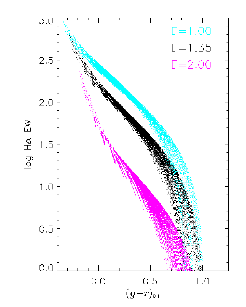
Figure 4: All model points for $\Gamma=1.00$ (cyan), $\Gamma=1.35$ (black) and $\Gamma=2.00$ (magenta). Each IMF has 18,480 calculated model values. $Z$ ranges from 0.005 to 0.025, ages range from 100 Myr to 13 Gyr and SFHs cover the range described in the text.

Figure 4 shows all 18,480 model points with $\Gamma=1.35$. Models are interpolated in SFH history for fuller coverage of the color-H$\alpha$ EW plane. For each value of $\Gamma$ the models cover a stripe rather than a single line. It can be seen in the lower right of figure 4 that the model become degenerate in $\Gamma$ for old, red galaxies with weak current star formation.

5 Statistical Techniques

The data and models are compared using a “pseudo-$\chi^{2}$” minimization. For various reasons (detailed below) the classical $\chi^{2}$ estimator assumptions are violated so we can not use traditional tables for error estimates but we can still use the $\chi^{2}$ as a statistical estimator as long as the confidence regions are calibrated by Monte Carlo (MC) techniques as we will do. We proceed as follows: for each galaxy $i$ we have a measured $(g-r)_{0.1}$ color, $c_{i}$, and an H$\alpha$ EW, $w_{i}$, and measurement errors $\sigma_{c_{i}}$ and $\sigma_{w_{i}}$, given by equations 5 and 7. We also have model values $c(\Gamma,Z,\tau,\psi)$ and $w(\Gamma,Z,\tau,\psi)$ for a range of IMF slopes $\Gamma$, metallicities $Z$, ages $t$ and SFHs $\psi$. We can then construct a $\chi^{2}$ value as

$$\chi_{i}^{2}(\Gamma,Z,t,\psi)=\left(\frac{c_{i}-c(\Gamma,Z,t,\psi)}{\sigma_{c_{i}}}\right)^{2}+\left(\frac{w_{i}-w(\Gamma,Z,t,\psi)}{\sigma_{w_{i}}}\right)^{2}$$ (8)

which is calculated by brute force. The goal of this paper however is to investigate the IMF with relatively simple measurements of the H$\alpha$ EW and a broadband color. While making crude measurements of the mean stellar metallicities of individual galaxies is possible, disentangling age and SFH effects on an individual basis is a daunting task. Assuming that it is possible to do, it does not scale up well to the high redshift universe where observations will be of lower quality.

It does not make sense to minimize $\chi^{2}$ over all galaxies for a particular set of $(\Gamma,Z,t,\psi)$ because we have no a priori reason to think that all of the galaxies should have the same metallicity or SFH. In fact we expect that they would not. The solution is to marginalize $\chi^{2}$ over metallicity, age and SFH for each galaxy such that

$$\chi_{i}^{2}(\Gamma)=\min\left[\chi_{i}^{2}(\Gamma,Z,t,\psi)\right]_{Z,t,\psi}$$ (9)

This is somewhat unorthodox, because for some galaxies the data points are over-fitted, i.e. there will be a stripe in ($c,w$) space corresponding to a given $\Gamma$ and we can get $\chi^{2}_{i}(\Gamma)$ values very close to zero (but not exactly because of the discrete nature of the model grid) for galaxies within the stripe. We note we also have partial degeneracy between parameters such as age and metallicity — they both shift the tracks in similar directions largely orthogonal to $\Gamma$ (though not completely which is why we have a stripe in parameter space not a line). This makes it difficult to calculate the traditional “number of degrees of freedom.” Despite these limitations it is clear that galaxies inconsistent with a particular $\Gamma$ will still have large values of $\chi^{2}_{i}(\Gamma)$– for example a very blue galaxy with a low equivalent width in Figure 4. The complication is that the stripes for similar $\Gamma$ values overlap, and for red galaxies with low equivalent widths the stripes for vastly different $\Gamma$ values overlap. As such, the IMF for an individual galaxy is only broadly constrained. Measuring a precise best IMF for an individual galaxy boils down to random chance and the discrete nature of the models. However, by summing $\chi_{i}^{2}$ over many galaxies the IMF is narrowly constrained for the sample being summed over as long as we are careful in our confidence region analysis.

Because of this over-fitting and partial degeneracy we can not apply the textbook notions of the $\chi^{2}$ distribution, calculate degrees of freedom and choose $\Delta\chi^{2}$ contours for different confidence regions. Further to this $c_{i}$ and $w_{i}$ are not truly independent variables. Both the colors and EWs are subject to the same extinction and reddening corrections which tie the errors together. For galaxies with $z\lesssim 0.04$ the H$\alpha$ line is in the observed $r$ band, although this only affects a relatively small number of galaxies in the sample almost all of which have $M_{r,0.1}>-20$. Also the direct statistical interpretation of $\chi^{2}$ is predicated on the assumption of normal errors. Equations 5, 6 and 7 reveal that our errors are complicated mixtures of individual measurements which are most likely Poisson distributed. Thus $\sigma_{c}$ and $\sigma_{w}$ are unlikely to be normally distributed. Bursty SFHs can potentially create outliers which are statistically significant due to the fact that neither $\sigma_{c}$ or $\sigma_{w}$ include a term for this difficult to quantify effect. The problem is even worse if the errors are non-symmetric which could potentially arise from the aforementioned bursty SFHs. In the case of non-symmetric errors the best value of $\Gamma$ could erroneously be pulled away from the true value.

Given all this we abandon the direct statistical interpretation of $\chi^{2}$ and regard it as an estimator of the goodness of fit whose confidence regions have to be calibrated empirically. We do this via MC simulations (as recommended by Press et al. (1992)) where we simulate data points for a given $\Gamma$ with the correct error distributions and propagate everything through the analysis in the same way as for the actual data. For each of our MC simulations we add Poisson errors to the $ugriz$ fiber magnitudes, H$\alpha$ and H$\beta$ fluxes and the observed H$\alpha$ EW. We assume that these observed quantities have Poisson dominated errors– as members of the MGS they are high S/N measurements. The entire analysis described above is repeated, including a new extinction measurement and a recalculation of the $K$-corrections. For each value of $\Gamma$ we run 100 MC simulations to estimate the 95% confidence interval. Setting up the MC architecture in this way has the further advantage that we can use the same machinery to test the effect of systematic errors such as the violation of our smooth SFH assumptions, as we will do later. The main downside of course is that this approach is computationally intense. Run times for the 100 MC simulations are typically 18 days on a 2 Ghz desktop PC for the samples considered here.

In practice it turns out that $\chi^{2}(\Gamma)$ is still a smooth well-behaved function with, not surprisingly, a quadratic minimum which has the advantage that we can then interpolate it to increase the resolution in the best-fitting $\Gamma$ without incurring the additional computational expense. This arises of course from the fact that our estimator is similar to a traditional $\chi^{2}$ and is a good reason to stick with this similarity over some more exotic goodness of fit measure. An estimate of the systematic errors is discussed later.

Regardless of how poorly a sample is modeled by a universal IMF the above method will still find a best fitting $\Gamma$ and corresponding confidence region. We still expect $\chi^{2}$ to be small for a model that is a good fit and large for one that is not. One nuance in comparing $\chi^{2}$ between different sub-samples, as we will do, is that the samples are often of considerably different sizes. Because of this we choose instead to use the mean $\chi^{2}$, $\overline{\chi^{2}}$ instead, as a sample metric. This has the advantage that absolute $\overline{\chi^{2}}$ values and confidence regions are more similar between the sub-samples, though we note that the confidence regions on $\overline{\chi^{2}}$ are still determined directly from our MC simulations.

6 Monte Carlo Results

Figure 5 shows the results of our analysis for the full sample of galaxies using just the observed data set. The “X” marks the best fitting IMF, where $\Gamma=1.4411$ and $\chi^{2}=60549.7$ with $\overline{\chi^{2}}=0.46$. At $\Gamma=1.00$ $\overline{\chi^{2}}=3.61$ while steeper IMFs are more heavily rejected with $\overline{\chi^{2}}=9.00$ at $\Gamma=2.00$.

For comparison several “classic” IMFs are also plotted in figure 5 at their approximate equivalent values of $\Gamma$. With $\overline{\chi^{2}}=7.73$ the Miller & Scalo (1979) solar neighborhood IMF is a particularly bad fit. Two more recent solar neighborhood IMFs, Scalo (1986) and Kroupa, Tout, & Gilmore (1993), yield $\overline{\chi^{2}}=2.38$ and 1.98 respectively. These results reinforce the conclusions of K83, KTC94 and Baldry & Glazebrook (2003) that the solar neighborhood is not representative of galaxies on the whole as far as the IMF is concerned.

On the other hand the Scalo (1998) IMF, established from a review of star cluster IMF studies in the literature, is a better fit than the best $\Gamma$ value in our parameterization with $\overline{\chi^{2}}=0.43$. This result highlights the degeneracy of the IMF models themselves in the color-H$\alpha$ EW plane– two considerably different IMFs (one with one break and the other with two) fit nearly equally as well.

The results of the MC simulation show that the 95% confidence region is $1.4432<\Gamma<1.4443$ for the data set as a whole. The MC simulation shows that additional data will not improve the overall results as the random errors are already small. Clearly and not surprisingly systematic errors, which are discussed later, dominate.

The overall result of $\Gamma=1.4437\pm 0.0005$ is steeper than the original Salpeter value of $\Gamma=1.35$. It is also steeper than the Baldry & Glazebrook (2003) value of $\Gamma=1.15\pm 0.2$ derived from galaxy luminosity densities in the UV to NIR. It is however well within their 95% confidence limit of $\Gamma<1.7$ as well as their measurement of $\Gamma=1.2\pm 0.3$ based on the H$\alpha$ luminosity density. The difference between their two results suggests that the H$\alpha$ and mid-UV to optical fluxes may have different sensitivities to massive stars. Scalo (1998) estimated the uncertainty in $\Gamma$, either due to measurement uncertainties, real IMF variations or both, in his star cluster IMF based on the spread of results in the literature. Our result is well within his range of uncertainty in both mass regimes– $\Gamma=1.7\pm 0.5$ for $1-10\ {\rm M}_{\odot}$ and $\Gamma=1.3\pm 0.5$ for $1-100\ {\rm M}_{\odot}$.

6.1 Luminosity Effects

The luminosity of a galaxy could potentially have an effect on the IMF within it. For one the ambient radiation field is likely higher in more luminous galaxies. Figure 6 shows the best fitting IMF and $\overline{\chi^{2}}$ values as a function of ${\rm M}_{r,0.1}$ for all 130,602 galaxies. The galaxies have been binned in ${\rm M}_{r,0.1}$ such that there are 500 objects in each bin. The bin size was chosen to maximize coverage in ${\rm M}_{r,0.1}$ yet still keep the random errors in each bin small. The solid lines represent the lower and upper 95% confidence region determined from the MC simulation.

Figure 6 reveals a constant value of $\Gamma\sim 1.4$ for galaxies with ${\rm M}_{r,0.1}$ between $-21$ and $-22$ with linear increases in $\Gamma$ for both brighter and fainter galaxies. There is also a sudden downturn in $\Gamma$ values for galaxies fainter than ${\rm M}_{r,0.1}=-16.5$. Given the sizes of the random errors the differences in $\Gamma$ between ${\rm M}_{r,0.1}=-17$ and $-22$ are substantial, from 1.59 to 1.41, and statistically significant. The agreement with the Salpeter slope is the best for galaxies between $-21$ and $-22$ in ${\rm M}_{r,0.1}$.

In many ways it is not surprising that previous investigators have not found this trend. The Milky Way is thought to have a luminosity of ${\rm M}_{V}=-20.9$ (Delhaye, 1965); the $V$ and $r_{0.1}$ filter curves cover roughly the same wavelengths. At comparable luminosities our results are similar to Salpeter. The galaxies in the K83 sample have a median ${\rm M}_{B}=-20.9$ with only 16% (18 objects) fainter than ${\rm M}_{B}^{*}=-19.7$ (Efstathiou, Ellis, & Peterson, 1988). This is a significant bias toward more luminous galaxies where our results are in agreement with a universal IMF. By contrast 30% of our sample is fainter than ${\rm M}_{r,0.1}^{*}=-20.44$ (Blanton et al., 2003b). We have a sample of 39,350 galaxies fainter than $\rm{L}^{*}$.

The lower panel of Figure 6 shows that the relative quality of the fits rapidly deteriorates as the luminosity of the galaxies decrease. For the brightest galaxies $\overline{\chi^{2}}$ floats around 0.15, while in the faintest bin it is over 6. For comparison ${\rm M}_{V}=-18.5$ for the Large Magellanic Cloud and $-17.1$ for the Small Magellanic Cloud (Courteau & van den Bergh, 1999). This trend could indicate that a universal IMF is a good fit to the most luminous galaxies, but dwarf galaxies cannot be described by a universal IMF, even if a different universal slope is allowed. However it could have a more mundane explanation. It could be that errors are over or underestimated as a function of luminosity. It also could arise from deviations from our assumption of smoothly varying SFHs.

We cannot bin our data by stellar mass without assuming an IMF which is contrary to the goals of the project. We can repeat the analysis of Figure 6 using ${\rm M}_{z,0.1}$ in the place of ${\rm M}_{r,0.1}$. ${\rm M}_{z,0.1}$, being redder, is a better proxy to stellar mass. The resulting plot is nearly identical to Figure 6 which shows that the relationship persists across several wavebands.

Figure 6 reveals a clear, statistically significant trend in $\Gamma$ and $\overline{\chi^{2}}$ with respect to luminosity. The rest of this section focuses whether this trend is a manifestation of true IMF variations or if it is the result of sample biases or poor assumptions.

6.2 Sources of Bias

If the IMF is truly universal and our method successfully probes the IMF any subsample of galaxies that we could choose should yield the same $\Gamma$ value as any other in spite of any selection biases or aperture effects. Figure 6 clearly shows that the preceding statement is false. In this section we set aside the possibility of IMF variations and search for biases in our sample.

6.2.1 Magnitude Limited Sample

Figure 6 shows that the overall result of $\Gamma=1.4437$ is really a weighted average. The SDSS MGS is a magnitude limited sample, one defined by flux limits, with both upper and lower limits. Table 1 gives the number of objects in each luminosity bin. There are 41,411 galaxies with $-21.5<{\rm M}_{r,0.1}<-20.5$ but only 28 for which $-14.5<{\rm M}_{r,0.1}<-13.5$. As such the overall result is heavily biased by more luminous galaxies.

Malmquist bias will affect any magnitude limited sample. Because brighter objects can be seen at greater distances a magnitude limited sample contains bright objects from a greater volume of space than fainter objects. The result is that the ratio objects by luminosity in a magnitude limited sample differs from the true ratio in nature; brighter objects are over-represented.

To eliminate Malmquist bias volume limited bins where subsamples are complete for a range of luminosities are constructed. Figure 7 details the construction of these bins. Given both the upper and lower flux limits of the MGS ($15.0<r<17.77$) only a factor of 13 in luminosity falls in the sample at any given redshift. The redshift limits of each volume limited bin are defined such that no galaxies within the magnitude limits of the bin are affected by the flux limits of the MGS. Within each box in Figure 7 the true ratio of galaxy luminosities is preserved and is thus free of Malmquist bias.

Figure 8 shows the results for volume limited magnitude bins. Most error bars are smaller than the plotting symbols due to the larger number of galaxies, 329 to 29,701 as given in Table 1, in each bin. Figures 6 and 8 show the exact same trends. The largest difference in $\Gamma$ between the whole and volume limited samples is 0.0116 in the ${\rm M}_{r,0.1}=-17$ bin. The other notable difference is that the fainter galaxies have larger $\overline{\chi^{2}}$ values in the volume limited case. However Malmquist bias across bins is not responsible for the luminosity trends in Figure 6.

6.2.2 Redshift

Another effect of magnitude limited samples is that the faintest galaxies are much closer than the most luminous ones. The mean redshifts of the volume limited magnitude bins range from $z=0.013$ for ${\rm M}_{r,0.1}=-17$ to $z=0.168$ for ${\rm M}_{r,0.1}=-23$. This corresponds to a difference in age of around 1.8 Gyr. As aforementioned, model tracks reveal that age is largely orthogonal to the IMF in our parameter space, but there could be other effects tied to age and distance. In addition the IMF could evolve with time.

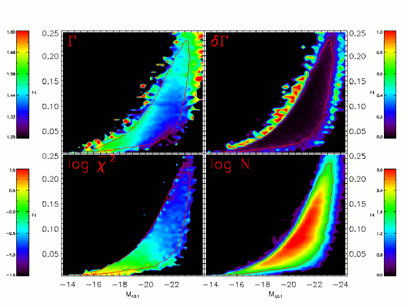
Figure 9: Values of fitted parameters as a function of both luminosity and redshift. The bins extend 0.25 magnitudes in luminosity and 0.005 in redshift. Clockwise from upper left the frames show the best fitting $\Gamma$, the width of the 95% confidence region in $\Gamma$ from the MC simulation, the log of the number of galaxies in each two dimensional bin and the log of $\overline{\chi^{2}}$. The shading levels for each panel are given by the adjacent vertical color bars. Black areas indicate regions where there are no galaxies with the respective combination of redshift and luminosity. The red contour indicates the region in which there are at least 50 galaxies in each 2-D bin.

The large number of galaxies in our sample affords us the luxury of investigating the effects of luminosity and redshift simultaneously to obtain a better understanding of what role, if any, the redshift plays in our analysis. Figure 9 shows our fitted parameters for all 130,602 galaxies in bins that are 0.25 magnitudes wide in luminosity and 0.005 wide in redshift. The upper left panel shows the best fitting $\Gamma$ for each two dimensional bin. On the upper right the width of the 95% confidence region in $\Gamma$ for each bin is shown. At bottom left is the $\log\overline{\chi^{2}}$ and at bottom right is the log of the number of galaxies in each bin. The white contour demarcates the region in which each bin contains at least 50 galaxies. The number 50 is arbitrary but it shows the region where Poisson errors are expected to be small. The black areas are regions where there are no galaxies with the given parameters.

Using the plot of $\Gamma$ at the upper left we can look for potential redshift biases. This is complicated by the fact that at a fixed luminosity there is a limit to the range of redshifts in the sample due to the flux limits of the sample described earlier. Looking at vertical slices through the plot at any fixed luminosity there is a trend towards larger values of $\Gamma$ with increasing redshift. However, for horizontal slices of fixed redshift the same relationship between $\Gamma$ and luminosity that is present for the whole sample is seen modulo a normalization factor.

The right half of Figure 9 shows a strong relationship between the number of galaxies per bin and the width of the 95% confidence region in $\Gamma$. This simply reflects the fact that larger samples are less affected by Poisson errors.

The lower left panel of Figure 9 provides an excellent example of why our metric of fit quality, $\overline{\chi^{2}}$, is so important. Bins with similar numbers of galaxies and $\delta\Gamma$ values can have vastly different values of $\overline{\chi^{2}}$. It is worth reminding that the contours in $\overline{\chi^{2}}$ are logarithmic. At fixed luminosity the galaxies are better fit by a universal IMF at higher redshift. Similar to the sample as a whole the quality of fit improves with luminosity.

While there does appear to be some weak trending of $\Gamma$ and $\overline{\chi^{2}}$ with redshift, redshift effects are not driving the relationship seen between IMF and luminosity as it persists at fixed redshifts.

6.2.3 Aperture Effects

One explanation for the trend in $\Gamma$ with redshift is aperture effects. Again, if the IMF is truly universal aperture effects should not exist. The SDSS spectra have a fixed aperture of 3” for all galaxies. Depending on the angular extent and distance to a galaxy a different fraction of the total light of the galaxy will fall into the aperture. The problem is mitigated by the fact that the most distant galaxies are the most luminous and more likely to have a larger physical size. As the physical area contained in the aperture increases with distance, so too does the size of the galaxies being observed. However, the two effects do not exactly balance out. Table 1 shows that the mean aperture fraction for the ${\rm M}_{r,0.1}=-17$ bin is 0.20 and increases to 0.27 at ${\rm M}_{r,0.1}=-23$. On average 35% more of the most luminous galaxies fall within the aperture compared to the faintest.

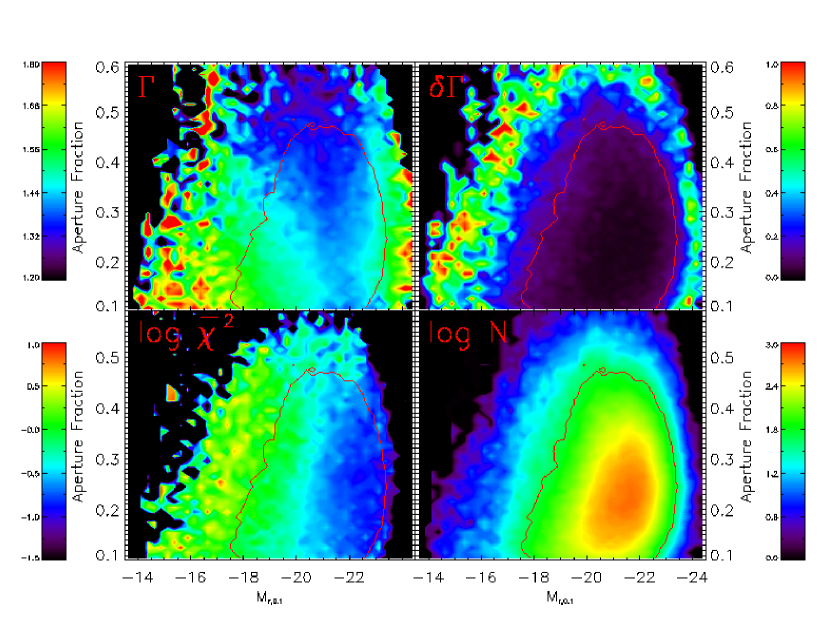
Figure 10: Values of fitted parameters for 2-D bins cut on luminosity and aperture fraction. The bins extend 0.25 magnitudes in luminosity and 1% in aperture fraction. The description is identical to Figure 9 as are the shading levels.

Figure 10 shows the behavior of our fitted parameters for two dimensional bins of luminosity and aperture fraction in the same manner as Figure 9 did for luminosity and redshift. For fixed luminosities increasing aperture fraction leads to decreasing values of $\Gamma$. However at fixed aperture fraction the qualitative IMF-luminosity trend remains. The $\overline{\chi^{2}}$ values are a strong function of luminosity, but $\overline{\chi^{2}}$ does increase with aperture fraction at each fixed luminosity.

The trend with aperture fraction is the exact opposite of what would be expected in the presence of a systematic effect operating given the redshift result in Figure 9. The nearest galaxies should have the smallest aperture fractions in a particular luminosity bin. The nearest galaxies in Figure 9 have the smallest values of $\Gamma$ while the smallest aperture fractions in Figure 10 have the largest values of $\Gamma$.

Figure 10 suggests that the measured IMF is more dependent on the aperture fraction than the redshift. There are several possible physical explanations for IMF trends with the aperture fraction, all of which are related to radial gradients in disk galaxies. Padoan, Nordlund, & Jones (1997) make the theory based claim that the IMF should be a function of the original local temperature of the star-forming molecular clouds. Metallicity gradients are also known to exist in disk galaxies, including the Milky Way (Mayor, 1976). Rolleston et al. (2000) measure a linear, radial light metal (C, O, Mg & Si) abundance gradient of $-0.07\pm 0.01\rm{\ dex\ kpc}^{-1}$ in the disk of the Milky Way. Given the increased efficiency of cooling with metal lines we would expect the most low mass stars where metallicity is the highest– on average towards the center of galaxies. The trend in $\Gamma$ in Figure 10 is qualitatively consistent with this idea.

If there are radial IMF gradients in galaxies one would expect the fits to decrease in quality with increasing aperture fraction. A blend of IMFs will not be fit as well as a universal one given our technique. This idea is consistent with the results in Figure 10. However, in well-resolved stellar populations there is no evidence for a relationship between the IMF and metallicity, except perhaps at masses lower than those probed by our method (Kroupa, 2002). If metallicity plays a role in determining the IMF the effects are only being revealed as a global trend in our large sample of integrated stellar populations. For individual clusters metallicity must play a secondary role to stochastic effects.

6.2.4 Extinction Correction

The extinction correction is another potential source of bias. It is possible that there is a second order correction that our fairly simple extinction correction fails to take into account. This could potentially lead to an erroneous IMF trend with extinction correction. This affects the luminosity results because more luminous galaxies tend to be dustier, as evidenced in Table 1. The problem is further complicated by the fact that dust is thought to play an integral part in star formation so it is not unreasonable that an observed IMF trend with extinction may be real.

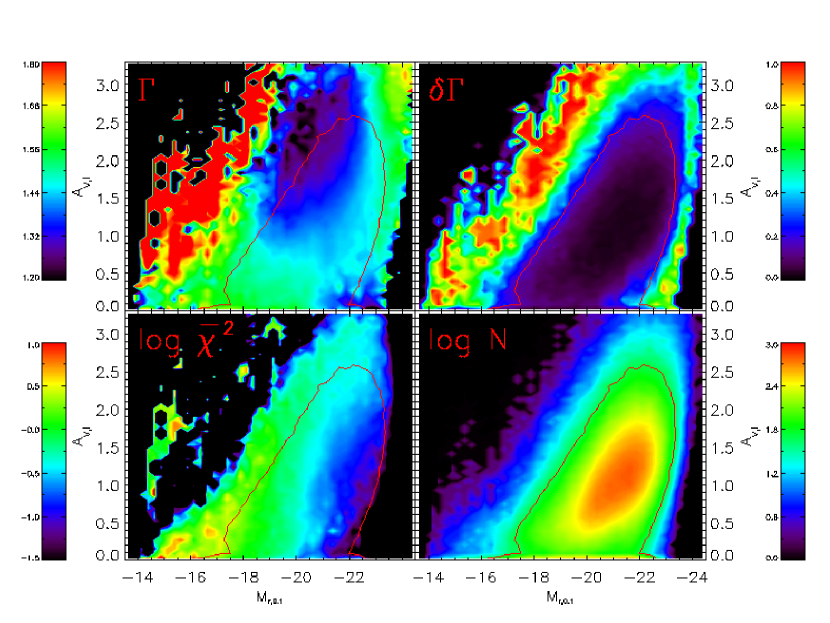
Figure 11: Values of fitted parameters for 2-D bins cut on luminosity and emission line extinction. The bins extend 0.25 magnitudes in luminosity and 0.06 magnitudes in extinction. The description is identical to Figures 9 and 10, as are the shading levels.

Figure 11, similar to Figures 9 and 10, shows the results of our analysis for two dimensional bins of luminosity and the extinction correction that was measured and applied. Vertical slices through the upper left panel of Figure 11 show that $\Gamma$ does depend on ${\rm A}_{{\rm V},l}$, trending towards lower $\Gamma$ values with increased extinction over the region where the Poisson error in $\Gamma$ is reasonable. Yet again, horizontal cuts of fixed extinction show the IMF-luminosity relationship.

The decreasing $\Gamma$ values with increasing extinction is counter-intuitive. Dustier regions tend to be more metal rich. If metal cooling plays a significant role in the IMF the dustiest regions should have the steepest IMFs.

At fixed luminosity $\overline{\chi^{2}}$ increases with extinction. As aforementioned our calculated errors in color and EW (equations 5 and 7) have a functional dependence on the observed emission line extinction. In both cases it is the term proportional to $\sigma_{f}{{\rm A}_{{\rm V},l}}$ which is on average the major contributor to the calculated error. Because luminous galaxies tend to be more heavily extincted they will also be more likely to have larger errors. This is potentially problematic for our observed IMF trend with luminosity. If we are unknowingly underestimating the errors for faint galaxies with low extinction the source of the poor fit qualities of these galaxies could be systematic instead of astrophysical. However the lower left panel of Figure 11 shows that the most extincted galaxies have the poorest fits where such a bias would suggest that they should fit the best due to the large accommodating errors.

6.2.5 Multiple Parameter Biases

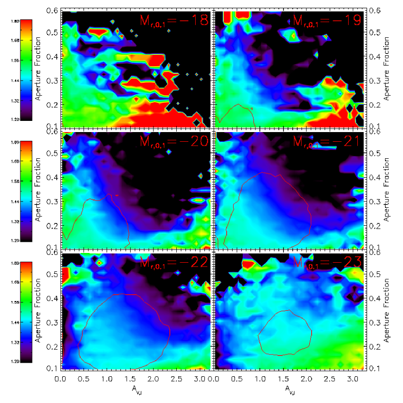
Figure 12: Best fitting $\Gamma$ values as a function of aperture fraction and measured emission line extinction for six volume limited luminosity bins. The 2-D bins extend 0.1 magnitudes in extinction and 2% in aperture fraction. The volume limited bins are defined as described in Figure 8. The red contour shows the area where the 2-D bins contain at least 50 galaxies. The shading levels are described by the color bars on the left.

It is also possible that biases in our $\Gamma$ measurements could depend on two parameters simultaneously. Figure 12 shows the measured galaxy of $\Gamma$ as a function of both aperture fraction and measured emission line extinction for six volume limited luminosity bins.

When holding all other parameters fixed, increasing the aperture fraction leads to lower values of $\Gamma$ in all statistically significant areas of Figure 12. This is the same relationship found in the earlier section on aperture fraction. Decreasing values of $\Gamma$ are also seen for increasing extinction when all other parameters are constant. A notable exception to this is that galaxies with large extinction and small aperture fractions favor higher $\Gamma$ values.

Most importantly when looking at a particular combination of aperture fraction and extinction the IMF becomes shallower with increasing luminosity until the highest luminosities where it becomes steeper again. Even in the narrowest slices of the data set the same IMF-luminosity trend is seen, albeit with slightly different absolute values of $\Gamma$.

6.2.6 Star Formation Strength

As discussed previously we have allowed two classes of star forming galaxies into our sample. 111,806 galaxies (86%) fall in the star forming class and the other 18,796 (14%) belong to the low S/N star forming class where the O III or N II lines are weak, but the H$\alpha$ and H$\beta$ lines still have S/N $>5$. By comparing the results from these two subsamples we can investigate a possible bias of the results with respect to the level of star formation.

Figure 13 shows the results for both classes as a function of luminosity. As it comprises 86% of the total sample it is not surprising that the results for the star forming class are similar to those of the sample as a whole in Figure 6.

The low S/N class exhibits a similar qualitative behavior to the set as a whole with a few notable differences. The $\Gamma$ values are offset by at least 0.08 towards larger $\Gamma$. The measured IMF turns toward steeper values at lower luminosities than for the sample as a whole. The $\overline{\chi^{2}}$ are several times lower as well.

While the galaxies in low S/N class meet the same requirement of S/N $>$ 5 in the Balmer lines as the star forming class they are biased towards noisier H$\alpha$ line measurements. This corresponds to lines that are either weak (low SFR) or weak compared to the continuum (low present SFR compared to the past) both of which lead to low EWs. Another issue at play is that the relationship between the H$\alpha$ line flux and the SFR is dependent on the IMF. At a fixed metallicity and SFR increasing $\Gamma$ by 0.05 reduces the H$\alpha$ flux by 20%. In fact the H$\alpha$ flux of a galaxy with $\Gamma=1.00$ will be 33 times larger than a galaxy with the same SFR and $\Gamma=2.00$. In the presence of real IMF variations at any fixed luminosity the low S/N class will be biased towards galaxies with steeper IMFs. Both low SFRs and steep IMFs potentially lead to low S/N H$\alpha$ flux. However it is difficult to determine the level of influence of each effect.

As shown in figure 1 low H$\alpha$ EWs lead to larger values of $\Gamma$ for any fixed color. As the low S/N class tends toward noisier H$\alpha$ fluxes and therefore EWs it is easy to see from equations 5, 6 and 7 that the errors for this class will tend to be larger. This in turn leads to lower $\chi^{2}$ values.

As the qualitative IMF-luminosity trend occurs in both star forming classes the strength of star formation is unlikely to be a significant bias on our results.

6.2.7 The $f$ Ratio

As mentioned in the data corrections section, the $f$ ratio is ratio of the extinction experienced by the nebular emission lines to that experienced by the stellar continuum. The assumption of a value for $f$ could potentially bias our results. An alternative way of looking at the same problem is that our data in the color-H$\alpha$ EW plane can be used to constrain the $f$ ratio by assuming a universal Salpeter IMF.

Figure 14 gives the results of this analysis for the data set as a whole. A value of $f=2.0$ is found with $\overline{\chi^{2}}=1.068$. This is in good agreement with to the Calzetti, Kinney, & Storchi-Bergmann (1994) value of $f=2.0+0.6/-0.4$. The quality of the fit in the best case is worse than in Figure 5. Part of the reason for this is that the errors used were slightly smaller as the $\sigma_{f}$ terms in equations 5 and 7 are set equal to 0. The quality of the fit drops sharply below $f=2$ and more gradually for $f>2$. Values of $f$ near 1 are heavily rejected. However in this particular plot the results are dominated by luminous galaxies.

The values of $f$ as a function of luminosity are shown in Figure 15. For galaxies ${\rm M}_{r,0.1}=-19$ and brighter the best value of $f$ is consistent with $f=2$. The faintest two bins the prefer an $f$ ratio closer to 2.5. However the lower panel shows that this new $f$ value does not translate to improved fit quality. In fact the faintest galaxies have in general smaller measured extinctions and are therefore less susceptible to changes in $f$. The same qualitative trend of worsening fits with decreasing luminosity seen when allowing $\Gamma$ to float is seen with a varying $f$ value.

Together these two $f$ ratio plots provide a number of insights. For one it shows that our choice of the $f$ ratio is very sensible and provides an independent confirmation of other $f$ ratio measurements. The fact that our best fitting $\Gamma$ values are at least 0.05 above the Salpeter value cannot be reconciled by changing the geometry of the dust screen. It provides further evidence that the relationship between $\Gamma$ and luminosity is not a function of extinction or a byproduct of our extinction correction.

6.2.8 Summary

In this section we have investigated several possible sources of bias to account for our observed trend between the IMF and luminosity. Relationships between the IMF and redshift, aperture fraction, extinction and star formation strength have been uncovered. Two parameter biases were also found.

In all cases in narrow slices through the data where potential biases are held fixed the qualitative IMF-luminosity relationship appears. The parameters primarily act to offset the value of $\Gamma$ at a particular luminosity. The ratio of continuum to emission line extinction, $f$, was found to be a sensible choice and the results are not sensitive to small changes in this value.

There are two possible interpretations to the relationships between the IMF and potential biases. One is that they are systematic effects due to some problem with our measurement of $\Gamma$. The second is that they are real physical effects. It is not clear from the data which of these statements is more correct.

6.3 Star Formation History

In the previous section several possible sources of bias were investigated, but none were able to account for our observed trend in $\Gamma$ with luminosity or the inability of a universal IMF to fit low luminosity galaxies. Figure 16 shows the distribution in color-H$\alpha$ EW space for the least and most luminous bins, ${\rm M}_{r,0.1}=-17$ and $-23$. From this figure it is apparent that the most luminous galaxies lie roughly parallel to the IMF tracks while the faintest galaxies are more perpendicular to the tracks. In the low luminosity bin there are galaxies which are simultaneously blue and have low EWs. These galaxies are not consistent with a universal IMF with $\Gamma=1.35$ and as mentioned before are not consistent with a universal IMF with a different slope. In addition the faintest galaxies have the lowest extinctions they are the least sensitive to dust and $f$ ratio issues. Before concluding that this is evidence for IMF variations we must first consider whether our model assumption of smooth SFHs is justified.

6.3.1 Effects of Star Formation Bursts

The SFH of individual galaxies is the most problematic aspect of the K83 analysis. A sudden burst on top of a smoothly varying background will immediately increase the H$\alpha$ EW. This is due to the formation of O and B stars which indirectly increase the H$\alpha$ flux through processing of their ionizing photons. The new presence of O and B stars also makes the color of the galaxy bluer. Both of these effects are proportional to the size of the burst.

After the burst is over the H$\alpha$ EW is smaller and the colors are redder than they would be if the burst had not occurred. The H$\alpha$ EW drops because there is no longer an excess of O and B stars and their ionizing photons which reduces the H$\alpha$ flux to pre-burst levels. However there is now an excess of red giants due to the less massive stars from the burst leaving the main sequence. This increases the continuum around the H$\alpha$ line which further drops the EW in addition to making the galaxy colors redder. After enough time has elapsed after the burst the galaxy returns to the same position in the color-H$\alpha$ EW plane it would have occupied had no burst occurred, although it will have taken longer to get there.

Figure 17 gives one example of this cycle. A solar metallicity galaxy with $\Gamma=1.35$ and an exponentially decreasing SFH with $\tau=2.15$ Gyr experiences a burst of star formation at an age of 4.113 Gyr which lasts 250 Myr and forms 10% of the stellar mass. The black dots, spaced at 100 Myr intervals, show that comparatively more time is spent below the nominal track than above it. The peak H$\alpha$ EW is reached just 5 Myr after the start of the burst. If you happen to be observing the galaxy during the burst a shallower IMF will be measured (assuming a burst-free SFH), after the burst for 1 Gyr a steeper IMF will be measured and after that the effects of the burst largely disappear, although the galaxy will appear younger than it actually is.

Figure 18 gives the best fitting IMF slope from our analysis, which assumes no bursts, as a function of age for the galaxy in Figure 17. The jitter in the best fit $\Gamma$ values is due to the discrete nature of our model grid, and the fact that the model tracks for different IMFs run together at large ages. Within a 300 Myr period during and just after the burst the best fitting IMF slope is anywhere from $\Gamma=1.00$ to 1.95. This shows that even if a universal IMF exists the SFH can mimic a huge range of IMF models. Roughly 1 Gyr after the burst the measured IMF is back to its true value. A galaxy with a bursty SFH viewed at a random time will be biased toward a steeper IMF than what is the true IMF. While one model is not an exhaustive study of the effects of the SFH on IMF measurements it does give a good sense of what issues arise.

To eliminate this uncertainty we investigated cutting the sample on SFH. In order to detect a relative lack or excess of present star formation it is necessary to measure both the present and past star formation rates or at least be able to compare the two in some way. The problem lies in the fact that conversions of observables into star formation rates assume an IMF to do so. Our aim is to measure the IMF so we cannot make strong a priori assumptions about it. Instead of biasing or results from the start we fit all galaxies and then try to determine the affect of SFHs on our conclusions.

6.3.2 Single Burst Models

The simplest burst model is that of a single burst at a random time on top of our smooth exponential SFHs. A grid of 1000 SFHs was constructed by first selecting one of the 24 smoothly varying SFHs at random. A burst lasting 200 Myr was superposed on the SFH at a time selected uniformly at random over a range of 12.5 Gyr. The strength of the burst was randomly selected up to 40% of the total stellar mass, with preference given to smaller bursts. The colors and EWs of these SFHs were calculated at 1 Myr intervals over 12.5 Gyr for the IMFs $\Gamma=1.35$ and 1.80 and a fixed metallicity of $Z=0.01$. This metallicity choice is based on the luminosity-metallicity relationship in Tremonti et al. (2004) for $M_{r,0.1}=-17$ galaxies. Plotting these models in the color-H$\alpha$ EW plane shows that all observed data points are covered by either IMF.

To test whether the observed distribution of points in the ${\rm M}_{r,0.1}=-17$ bin can be explained by bursting SFHs the MC techniques of §5 were used. The models of §4 were replaced with the grid of single burst models. The 100 MC simulations were constructed as described earlier, but using only the 329 ${\rm M}_{r,0.1}=-17$ galaxies as a basis. The analysis yielded $\overline{\chi^{2}}=0.027$ for $\Gamma=1.35$ and $\overline{\chi^{2}}=0.020$ for $\Gamma=1.80$, both of which are over fits.

This shows than an individual galaxy can be fit with an arbitrary IMF given the freedom to choose a SFH. However, our advantage is that we have many galaxies and the distribution of the properties of the best fit models can be shown to be implausible.

Figure 19 demonstrates the problem with the single burst model. On the left of the figure the distribution of the best fitting burst strengths are plotted as a fraction of the total stellar mass formed. At right is the distribution of the best fitting times from the burst onset. For example, a galaxy which best fits a model with a burst at 1.000 Gyr at an age of 1.211 Gyr has a time from burst onset of 211 Myr. This measure is used because in an investigation of the effects of bursts the age relative to the burst is more important than the age given that the bursts occur at different, random times across the models.

For both $\Gamma=1.35$ and $\Gamma=1.80$ the number of objects best fit by a model prior to the burst is $11+3/-5$, or 3%, and are not plotted. In both cases the distributions of the best fitting ages and ages at which the burst begins are roughly uniform. Given this fact it is expected that half of the galaxies should be best fit by a pre-burst model. Furthermore the right hand panel shows sharp, significant discontinuities in the distribution of best fitting time from burst onset. Again, viewed at random times this distribution should be uniform but is highly peaked in the 25 Myr at the start of the burst and the 25 Myr just after the burst ends. In both cases the errors bars show that the discontinuities are significant. In the case of $\Gamma=1.35$, 3.5 times as many galaxies are in the 200 Myr after the burst ends than the 200 Myr during it and this 400 Myr accounts for 57% of all galaxies. Although our sample is $r$-band selected the stars in the 0.7 to 3 M_☉ range which dominate the red continuum in the red giant phase do not start to leave the main sequence for 300 Myr. The sharp increase in galaxies fit at 200 Myr after the burst cannot be due to a selection effect. Assuming a universal IMF this points to a strong coordination of SFHs across a population of galaxies unrelated in space. These arguments show that while a single burst model can fit the data extremely well, it does not do so in a physically self-consistent fashion.

6.3.3 Multiple Burst Models

To find a physical motivation for SFH models for low luminosity galaxies we look towards the Local Group. There have been a number of recent studies of the SFHs of local dwarf galaxies which use HST to get color-magnitude diagrams (CMD) of resolved stellar populations. The SFH is determined by fitting isochrones to the CMD. The sample here is biased by Local Group membership and by what galaxies have been observed to date. The galaxies mentioned here give a point of reference rather than a well-defined distribution of SFHs.

The blue compact dwarf (BCD) UGCA 290 was found to quiescently form stars over the past Gyr up until a ten-fold increase in SFR from 15 to 10 Myr ago which more recently has decreased to a quarter of its peak value (Crone et al., 2002). The dwarf irregular IC 1613, which is relatively isolated and non-interacting, was found to have SFR enhanced by a factor of 3 from 3 to 6 Gyr ago without evidence of strong bursts (Skillman et al., 2003). The dwarf irregular NGC 6822, also relatively isolated, is found to have a roughly constant SFH (Wyder, 2003). The BCD NGC 1705 is found to be gasping- a SFH marked by moderate activity punctuated by short periods of decreased star formation (Annibali et al., 2003). The authors also note that NGC 1705 is best fit by an IMF with $\Gamma=1.6$. NGC 1569 likely experienced three strong bursts in the last Gyr as well as a quiescent phase from 150 to 300 Myr ago (Angeretti et al., 2005).

Inspired by the preceding Local Group SFHs we constructed six SFH classes with multiple bursts. These SFH classes are described in Table 2. Each class starts with an underlying smooth SFH. SFHs #1 & 2 have no star formation, #3 & 4 have a constant SFH and #5 & 6 have exponentially decreasing SFHs like those previously described. Star formation discontinuities are then superimposed on top of the smooth SFHs. These discontinuities are in the form of increased (bursts) or decreased (gasps) star formation for periods of 200 Myr. The time and spacing of the discontinuities is random with the mean interval between bursts listed in Table 2.

For each SFH class described above we randomly generated 1,000 SFHs. Colors and EW widths were calculated for each SFH using $\Gamma=1.35$ and $Z=0.01$. According to the SDSS mass-metallicity relationship (Tremonti et al., 2004) galaxies at ${\rm M}_{r,0.1}=-17$ will on average have $Z=0.01$.

We then repeated our $\chi^{2}$ analysis with the 100 MC simulations of the ${\rm M}_{r,0.1}=-17$ galaxies in the same manner as for the single burst models. The results of our analysis for each of the six SFH classes are shown in Figure 20. SFH 5, the gasps on top of exponential SFHs, is the best fit with $\overline{\chi^{2}}=0.09$. Extended periods of no star formation punctuated by bursts (SFHs # 1 & 2) do not fit the data.

As was the case for the single burst models an unreasonable fraction of galaxies are best fit by SFHs in the 20 Myr immediately following a burst or the first 20 Myr of a gasp. If the SFH models are reasonable we should see roughly equal numbers of galaxies in each time bin. There is no reason why all of the low luminosity galaxies across the large volume of space in the SDSS footprint should have experienced coordinated bursts. However each panel of Figure 20 has at least 40% of the galaxies in one 20 Myr bin.

One explanation for this is that it is an artifact of our sample being selected in the $r$ band. However spectral synthesis models show that for instantaneous bursts of star formation the $r_{0.1}$ magnitude is brightest at the burst time and decays smoothly for a range of $\Gamma$. If anything it is more likely to catch galaxies during a burst rather than after or after a gasp instead of during one.

Regardless of the SFH model the presence of blue galaxies with low H$\alpha$ EW requires a recent discontinuity in the SFR for $\Gamma=1.35$. Based on the evolution of the $r_{0.1}$ band luminosity we expect to see a similar number of galaxies with excess H$\alpha$ EWs. The fact that these galaxies are missing shows that the discontinuous SFH models do not match our observations. Therefore IMF variations are a more likely explanation for the observed distribution of ${\rm M}_{r,0.1}=-17$ galaxies.

6.3.4 Recovering $\Gamma$ from Synthetic Data

As a last exercise the best fitting SFH models from the previous section can be run forward to see if the correct IMF can be recovered. For each SFH model grids 10,000 data points were chosen by selecting a random SFH and a uniformly distributed age. Normal errors were added using the error characteristics of the ${\rm M}_{r,0.1}=-17$ bin. This synthetic data was analyzed in the same fashion as the real data in the earlier sections. For the single burst models the recovered IMF models for $\Gamma=1.35$ and 1.80 were 1.34 and 1.79 respectively with best fitting $\overline{\chi^{2}}=$ 0.80 and 0.65. For SFH 5 the recovered IMF was also $1.34$ with $\overline{\chi^{2}}=1.5$. In all three cases the correct IMFs were recovered although the fit was worsened by by the burst activity. This reinforces the difficulty in producing enough blue, low H$\alpha$ EW galaxies to match the observed data with simple SFH models.

7 H$\delta_{\rm A}$ Absorption

In the previous sections we have expanded on the K83 method and exploited the H$\alpha$ and color information as much as possible. In the bias section we found that various possible biases do not fully explain either the increased values of $\Gamma$ or the poor fit to a single IMF in the lowest luminosity bins. In the SFH section we found that an arbitrary $\Gamma$ value coupled with a plausible SFH with bursts or gasps can account for the position of any individual galaxy in the color-H$\alpha$ EW plane. However taking the population of ${\rm M}_{r,0.1}=-17$ galaxies together necessitates an incredibly unlikely coordination of SFHs across the disparate group of objects. This points to the extraordinary conclusion that while the IMF may be universal across luminous galaxies, it is not in fact universal in low luminosity galaxies. Such an extraordinary claim would ideally be backed by extraordinary evidence. In this section we take a look beyond the K83 method for some reinforcement of our result.

The H$\delta$ absorption feature can be used to gain additional insight into the nature of stellar populations. H$\delta$ absorption is due to absorption lines form stellar photospheres. The Balmer absorption lines are most prominent in A stars and weaken due to the Saha equation for both hotter and cooler stars. As such the H$\delta$ absorption is a proxy for the fraction of light of a stellar population being supplied by A stars, and to a lesser extent B and F type stars. In a stellar population of a uniform age the H$\delta$ absorption will peak after the O and B stars burn out, but before the A stars leave the main sequence. For this reason the strength of H$\delta$ can be used help determine the age of a population or to detect bursts of star formation which occurred around 1 Gyr in the past.

Worthey & Ottaviani (1997) describes two different methods for measuring H$\delta$ absorption. The H$\delta_{\rm F}$ definition is tuned to most accurately measure the H$\delta$ absorption from F stars. The H$\delta_{\rm A}$ definition has a wider central bandpass to match the line profiles of A stars. They state that the H$\delta_{\rm A}$ definition is better to use for galaxies because it is less noisy in low S/N galaxies and velocity dispersion acts to widen absorption features. On the downside the narrower H$\delta_{\rm F}$ definition is much more sensitive to population age where it can be used. Worthey & Ottaviani (1997) observationally determines the range of H$\delta_{\rm A}$ values to be from 13 for A4 dwarf stars to -9 for M-type giant stars.

H$\delta_{\rm A}$ values can be measured from the SDSS spectra. Like the H$\alpha$ EW values our H$\delta_{\rm A}$ values come from Tremonti et al. (2004) instead of the SDSS pipeline.

Figure 21 compares the distribution of the H$\delta_{\rm A}$ values for the ${\rm M}_{r,0.1}=-17$ and ${\rm M}_{r,0.1}=-23$ luminosity bins. For reference recall that Figure 16 plots the color and H$\alpha$ EWs for these two bins. The difference between the high and low luminosity bins is clear. Gaussian profiles can be fit to both distributions. For the ${\rm M}_{r,0.1}=-23$ bin the standard deviation of the profile is twice as large as the measurement error in H$\delta_{\rm A}$ suggesting that the true distribution has a range of values. Assuming both the errors and underlying distribution are Gaussian the distribution of H$\delta_{\rm A}$ for the luminous galaxies is centered at H$\delta_{\rm A}=3.4$ with a standard deviation of 1.5. By contrast, the Gaussian fit to the ${\rm M}_{r,0.1}=-17$ bin has the same standard deviation as the median error in the galaxies. This is consistent with nearly all of the galaxies having H$\delta_{\rm A}=6.1$.

This shows that the fainter galaxies on average have significantly larger fractions of A-type stars amongst their stellar populations. It also shows a seemingly unlikely coordination of H$\delta_{\rm A}$ in the low luminosity galaxies, reminiscent of the earlier suggestion of coordinated SFHs. The question then becomes why?

For a possible explanation we look again to the models. Modeling the behavior of H$\delta_{\rm A}$ requires an extra step. The standard PEGASE.2 models do not have the required resolution to accurately measure the H$\delta_{\rm A}$ index. This is remedied with the use of the PEGASE-HR code (Le Borgne et al., 2004) which uses a library of echelle spectra of 1503 stars to calculate spectral synthesis models with R=10,000 over the range of 4000 to 6800Å. Using PEGASE-HR in the low resolution mode yields the same results as PEGASE.2, and the same input parameters are used for both codes. The models here are the same as those described earlier in the models section, but have been recalculated using PEGASE-HR to allow H$\delta_{\rm A}$ measurements.

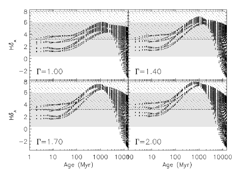
Figure 22: Model values of the H$\delta_{\rm A}$ index as a function of age for four IMF models, $\Gamma=1.00$ (upper left), 1.40 (upper right), 1.70 (lower left), and 2.00 (lower right). Each dot represents a model value for single IMF, metallicity, SFH (as described in the models section) and age. The four tracks identifiable towards the left of each panel are each of differing metallicities with the lowest metallicity models having the largest H$\delta_{\rm A}$ values at young ages. The grey area indicates the range of H$\delta_{\rm A}$ spanned by the middle 90% of the volume limited ${\rm M}_{r,0.1}=-23$ bin. The hashed area shows the middle 90% range for the volume limited ${\rm M}_{r,0.1}=-17$ bin.

Figure 22 shows the behavior of the H$\delta_{\rm A}$ index as a function of age for four different IMF models, $\Gamma=1.00$, 1.40, 1.70 and 2.00. For each IMF models of all metallicities and smooth SFHs are plotted for each age. The qualitative behavior of all models is the same. The H$\delta_{\rm A}$ holds steady for the first 20 to 40 Myr before increasing to a peak value at 700 Myr to 1 Gyr and then falls off. Prior to reaching the peak value for each IMF the metallicity has the strongest effect on the H$\delta_{\rm A}$ index. At this point the lowest metallicity galaxies have the highest H$\delta_{\rm A}$. After the peak the SFH has the strongest effect with the constant and increasing SFHs maintaining higher H$\delta_{\rm A}$ values.

After a few Gyr the differences in H$\delta_{\rm A}$ between models with different IMFs disappear. Prior to that there are three main differences. First, the peak H$\delta_{\rm A}$ values are higher for larger values of $\Gamma$. For $\Gamma=2.00$ H$\delta_{\rm A}$ reaches a maximum value of nearly 8 and the maximum value is similar for all metallicities. For $\Gamma=1.00$ the maximum value ranges from 4.5 to 6 depending on the metallicity. This is due to the fact that the steeper IMFs have fewer luminous massive stars to dilute the H$\delta$ absorption features from the A star population. Secondly, the low $\Gamma$ models have H$\delta_{\rm A}$ values that start their initial increases at a later time. Lastly the low $\Gamma$ models reach their peak values later in time than those with fewer massive stars.

To compare the H$\delta_{\rm A}$ values for the ${\rm M}_{r,0.1}=-23$ and $-17$ bins to the models the range of the middle 90% values from Figure 21 for each bin are overlaid on Figure 22. Once again the ${\rm M}_{r,0.1}=-23$ bin is in good agreement with our assumption of a universal IMF and smooth SFH. The range of H$\delta_{\rm A}$ values can be accomplished with a single Salpeter-like $\Gamma=1.40$ IMF with only the proviso that most galaxies be older than a few Gyr or younger than 300 Myr. However the exact same statement can be made for $1.0<\Gamma<2.0$ so H$\delta_{\rm A}$ provides only a constraint on the age of the most luminous galaxies, but not the IMF.

For the ${\rm M}_{r,0.1}=-17$ galaxies the distribution of H$\delta_{\rm A}$ cannot be achieved with the shallowest IMFs investigated under the assumption of smooth SFHs. However Salpeter and steeper IMFs can be accomplished. What changes is the range of ages over which the models have the correct H$\delta_{\rm A}$. Steeper IMFs require that the galaxies be either older than a few Gyr or 200 Myr old to accommodate the observed H$\delta_{\rm A}$ values. Most troubling is that there does not appear to be any reason why H$\delta_{\rm A}$ should stack up at 6.1 for the ${\rm M}_{r,0.1}=-17$ galaxies.

H$\delta_{\rm A}$ values can also be calculated for the same SFH class models used earlier. Unfortunately this does not provide any added constraints. H$\delta_{\rm A}$ values remain elevated for several 100 Myr after the start of a burst or the end of a gasp of SFH. The behavior of H$\delta_{\rm A}$ in the presence of SFH discontinuities provides no need for galaxies to stack up in the narrow 20 Myr intervals seen in the earlier multiple burst section, nor do these models suggest why the low luminosity galaxies are consistent with a single value of H$\delta_{\rm A}$.

There is no satisfactory model to account for the H$\delta_{\rm A}$ distribution of the low luminosity galaxies. However the SFH results from the previous section strongly suggest that the incredible coordination of discontinuities is highly unlikely. Steeper IMFs do allow for higher H$\delta_{\rm A}$ values for longer periods of time, thus relaxing the SFH coordination requirement. This agrees with our earlier results for faint galaxies. The low luminosity galaxies are most likely the result of a mix of IMFs which are on average steeper than Salpeter.

8 Conclusions

The goal of this paper was to revisit the K83 method for inferring the IMF from integrated stellar populations and to harness the richness of the SDSS data, improved spectral synthesis models and greater computational power available today to make a state-of-the-art measurement of the IMF. The quality of the SDSS spectroscopy allowed us to address several of the limitations of K83 and KTC94– we resolve the [N II] lines (a significant improvement in the accuracy of the H$\alpha$ EWs of individual galaxies), eliminate contamination from AGN, make extinction corrections for individual galaxies and fit underlying stellar absorption of H$\alpha$. We succeeded in achieving more accurate EWs for individual galaxies. The median total EW error for our sample is 17% compared to a 10% uncertainty in EWs combined with a 20-30% uncertainty in the extinction correction for K83.

We expanded the grid of models to allow for a range of ages and metallicities. We used $\chi^{2}$ minimization to go beyond differentiating between two or three IMF models to actual fitting for the best IMF slope. The vast size of the SDSS sample allowed us to both drive down random errors and to cut the data into narrow parameter ranges which were still statistically viable.

The size of the DR4 sample yielded $\Delta\Gamma=0.0011$ 95% confidence region due to random error for the sample as a whole. Even the volume limited ${\rm M}_{r,0.1}=-17$ luminosity bin with only 329 objects has a random error of $\Delta\Gamma=0.0086$. Only in bins with fewer than 10 objects do the random errors become significant. Our IMF fitting is therefore dominated by systematics.

Originally we believed that our systematics would be dominated by the effects of SFH discontinuities. However we conducted several experiments where we selected populations of galaxies from models with bursting or gasping SFHs and gave them measurement errors consistent with those in the ${\rm M}_{r,0.1}=-17$ luminosity bin. To our surprise our $\chi^{2}$ minimization revealed the true IMFs with $\Delta\Gamma=0.01$. The main effect was to reduce the quality of the fits. This is due to the fact that H$\alpha$ EWs return to nominal levels in a relatively short time after SFH discontinuities.

Another way to estimate the size of the systematic errors is to look at the trends of the ${\rm M}_{r,0.1}=-21$ and $-22$ luminosity bins, because they have the largest membership, in Figures 9, 10 and 11. Assuming that the IMF is universal and that our method is perfect we should get the same answer for any subset of the data we might choose. The largest ranges are $\Delta\Gamma\sim 0.12$ for redshift binning, $\Delta\Gamma\sim 0.19$ by aperture and $\Delta\Gamma\sim 0.19$ by extinction. Conservatively then the systematic error is $\pm 0.1$.

There are two points to be kept in mind about this estimate of the systematic error. For one it is the systematic error in the exact value of $\Gamma$. Even in Figure 12 where more narrow bands of measured extinction and aperture fraction are considered the same trends with luminosity are seen as with the sample as a whole. The relative systematics between luminosity bins in these narrow slices is much smaller. The second thing to remember is the way in which we empirically defined our systematic error discounts the possibility of IMF variations. What we have called systematics could actually be science. If galaxies have radial IMF gradients or if dust content plays a strong role in star formation the systematic error could be much smaller. The main area in which we were unable to improve upon the K83 and KTC94 studies is that they were able to match the aperture size to the galaxies which avoids the issue of aperture effects.

In spite of a more quantitative approach, like K83 and KTC94 the results are mostly qualitative. However there are four key results from our investigation.

First, for galaxies brighter than ${\rm M}_{r,0.1}\sim-20$ the best fitting IMFs are Salpeter-like ($\Gamma\sim 1.4$). In addition the assumption of a universal IMF and smoothly varying SFHs is a good fit. This is reassuring as it follows the conventional wisdom and provides confidence that the method works.

Secondly, galaxies fainter than ${\rm M}_{r,0.1}\sim-20$ are best fit by steeper IMFs with larger fractions of low mass stars. For these galaxies a universal IMF and smooth SFH is a poor assumption. This result is in qualitative agreement with evidence that LSBs have bottom-heavy IMFs (Lee et al., 2004).

Thirdly, while breaking the IMF-SFH degeneracy for individual galaxies using the H$\alpha$ EW and color is hopeless, for a statistical sample of galaxies the degeneracy can be broken.

Lastly, given our analysis of discontinuous SFHs it appears that the IMF is not universal in low luminosity galaxies and fewer massive stars are being created in these galaxies.

It is worth mentioning the main caveat of our $\Gamma$ values again. As illustrated in Figure 2 IMF parameterizations are themselves degenerate in our parameter space. Increasing the IMF slope has a similar effect to lowering the highest mass stars that are formed or increasing the fraction of intermediate mass stars. This method cannot explicitly determine if two populations have the same underlying IMF. Figure 5 shows that for the sample as a whole the Scalo (1998) three part power law yields nearly the same result as our two part power law. However our method is sensitive in many cases if the IMFs are different.

In terms of star forming cloud temperatures the harsher ambient radiation and larger number of sources of cosmic rays present in more luminous galaxies agree qualitatively with our results. With the extra energy hitting the star forming clouds larger masses may be needed for contraction and fractionization may end sooner, suppressing the formation of less massive stars (Larson, 1998). Cedrés, Cepa, & Tomita (2005) find that while the H II regions of the luminous grand design spiral NGC 5457 (M 31) can be reproduced by a single Salpeter IMF, for the low luminosity flocculent galaxy NGC 4395 a blend of two IMFs is required. However, such trends are not seen in studies of well-resolved stellar populations (Kroupa, 2002).

Another explanation for the absence of massive stars is that the massive stars are there, but are not visible. Extinction to the center of star forming regions, where massive stars preferentially exist, can reach ${\rm A_{V}}\sim 20$ (Engelbracht et al., 1998). However the low luminosity galaxies have the lowest observed extinctions (see Table 1) which is the opposite of what would be expected given our IMF results.

It is also possible that the IMF is in fact universal, but the way in which it is sampled in embedded star clusters leads to an integrated galaxial IMF which varies from the true IMF. Weidner & Kroupa (2005) use a universal IMF with the assumption that stars are born in clusters where the maximum cluster mass is related to the star formation rate. For a range of models this leads to a narrow range for the apparent IMF in high mass galaxies. For low mass galaxies the IMF is steeper with a wider range of slopes. The results here are in qualitative agreement for some of the integrated galactic IMF scenarios in Weidner & Kroupa (2005) given that there should be a rough correlation between galaxy luminosity and mass. Once again, Elmegreen (2006) argues that the galaxy wide IMF should be the same as the IMF in clusters regardless.

In light of the theory of Weidner & Kroupa (2005), whether the results of this paper speak to a relationship between environment and the formation of individual stars is open to interpretation. However the impact on the modeling and interpretation of the properties of galaxies is clear. Köppen, Weidner, & Kroupa (2007) note that the integrated galaxial IMF is the correct IMF to use when studying global properties of galaxies. Even if the IMF of stars is in truth universal it may currently be misused in the modeling of galaxies. Furthermore a varying integrated galaxial IMF could open the door to new insights in galaxy evolution. For instance, Köppen, Weidner, & Kroupa (2007) suggest that the observed mass-metallicity relationship in galaxies naturally arises from a variable integrated galaxial IMF similar to the results of this paper.

Future work will expand in several directions. The success constraining the IMF with only two observed parameters (albeit carefully chosen to be orthogonal to systematic errors) motivates a more expansive analysis with more parameters. Information from wavelength regimes beyond the SDSS can be used. For instance the absorption strength and P-Cygni profile shape of the C IV $\lambda 1550$ line due to massive stars is sensitive to the IMF slope and upper mass cutoff (Leitherer, Robert, & Heckman, 1995). However it could be contaminated by absorption from the interstellar medium and would need to be disentangled (Shapley et al., 2003). A full Markov Chain Monte Carlo analysis could be implemented fitting to multiple spectral features and marginalizing over a range of SFHs. In addition to luminosity, surface brightness and gas phase metallicity can be tested for systematic IMF variations. While the results for luminous galaxies are already dominated by systematics, the continued progress of the SDSS can provide better statistics for a more detailed analysis of what physical processes are behind the IMF variations in faint galaxies.

Table 1: Luminosity Bin Details

	Volume Limited								All
${\rm M}_{r,0.1}$	$n$	$\Gamma_{\rm low}$	$\Gamma_{\rm best}$	$\Gamma_{\rm high}$	$\overline{\chi^{2}}$	$\overline{z}$	$\overline{{\rm A}_{{\rm V},l}}$	$\overline{\rm ap}$	$n$	$\Gamma_{\rm best}$	$\overline{\chi^{2}}$
-14	-	-	-	-	-	-	-	-	28	1.3835	7.43
-15	-	-	-	-	-	-	-	-	188	1.3892	9.86
-16	-	-	-	-	-	-	-	-	406	1.5461	4.64
-17	329	1.6000	1.6045	1.6086	3.41	0.013	0.38	0.20	1,304	1.5879	2.57
-18	1,555	1.5338	1.5370	1.5424	2.05	0.022	0.50	0.21	4,327	1.5326	1.57
-19	4,935	1.4772	1.4788	1.4813	1.17	0.032	0.70	0.21	10,375	1.4813	0.96
-20	12,951	1.4306	1.4320	1.4330	0.63	0.050	0.91	0.22	24,851	1.4436	0.56
-21	28,633	1.4051	1.4057	1.4063	0.32	0.077	1.15	0.24	41,411	1.4064	0.31
-22	29,701	1.4036	1.4042	1.4050	0.19	0.116	1.32	0.25	38,406	1.4084	0.20
-23	8,049	1.4545	1.4556	1.4568	0.15	0.168	1.55	0.27	9,106	1.4505	0.16
-24	-	-	-	-	-	-	-	-	192	1.5329	0.12
All*	130,602	1.4432	1.4437	1.4443	0.50	0.090	1.05	0.25	-	-	-

Note. — Properties of the ${\rm M}_{r,0.1}$ luminosity bins. Columns 2 through 9 give values for volume limited magnitude bins while columns 10, 11 and 12 give values for all sample galaxies within the luminosity range. $\overline{\rm ap}$ is the mean aperture fraction. * The sample as a whole is not volume limited but the more detailed information is given for reference.

Table 2: Multi-burst SFH Models

Name	Type	Length	Relative	Spacing	Underlying
		(Myr)	Strength	(Gyr)	SFH
SFH 1	burst	200	-	3	none
SFH 2	burst	200	-	1	none
SFH 3	burst	200	4.0	3	constant
SFH 4	gasp	200	0.0	1.5	constant
SFH 5	gasp	200	0.1	1.5	exponential
SFH 6	burst	200	5.0	1.5	exponential

Figure 1: Distribution of all 130,602 program galaxies in the $(g-r)_{0.1}$ vs. $\log(\rm{H}\alpha\rm{\ EW})$ plane. The contours are logarithmic. Outside the last contour individual points are plotted. The thick lines are model tracks with exponentially decreasing SFHs with $\tau=1.1$ Gyr and solar metallicity. The age increases along the tracks from 100 Myr in the upper left to 13 Gyr in the lower right. The upper line has $\Gamma=1.00$, the middle line is similar to Salpeter’s IMF with $\Gamma=1.35$ and the lower line has $\Gamma=2.00$. They are identical to the solid lines in Figure 3. The cross in the lower left indicates the median error bars of the sample. The arrows are dust vectors are for typical observed Balmer decrements (H$\alpha$/H$\beta$ = 4) for different values of $f$. The values of $f$ are 1, 2 and 4 clockwise from the one pointing left.

Figure 2: Examples of the degeneracy of IMF parameters. All models shown have solar metallicity, age 6 Gyr and the tracks are lines of varying SFH from a rapidly decreasing SFR on the lower right to slowly increasing on the upper left. In both panels the bold track has $\Gamma=1.35$ and the dashed lines have IMFs $\Gamma=$ 1.00, 1.20, 1.40, 1.60, 1.80 and 2.00 from top to bottom, all with an upper mass cutoff of 120 M_☉. (a) The solid lines are models where the upper mass cutoff of the IMF is reduced from 120 M_☉ to 90, 60 and 30 M_☉ as labeled. (b) The nominal two-piece IMF is replaced by a three piece IMF in the solid lines. In all solid tracks $\Gamma=1.35$ above 10 M_☉ and $\Gamma=0.50$ below 0.5 M_☉, but is altered in the intermediate mass region from 0.5 to 10 M_☉. The solid lines have $\Gamma_{i}$ = 0.50, 0.85 and 1.15 over 0.5 to 10 M_☉ as labeled.

Figure 3: Effects of model parameters in the $(g-r)_{0.1}$ vs. $\log(\rm{H}\alpha\rm{\ EW})$ plane. In both panels ages of the stellar population increase along the tracks from 100 Myr on the upper left to 13 Gyr on the lower right. Also in both panels the upper set of tracks have $\Gamma=1.00$ while the lower set have $\Gamma=2.00$. The arrows are dust vectors are for typical observed Balmer decrements (H$\alpha$/H$\beta$ = 4) for different values of $f$. The values of $f$ are 1, 2 and 4 clockwise from the one pointing left. (a) The effect of smooth SFH variation is shown in the left panel. The solid lines have exponentially decreasing SFRs with $\tau=1.1$ Gyr, the dotted lines have more slowly falling SFRs with $\tau=2.75$ Gyr and the dashed lines are increasing $\propto 1-e^{-t/\tau}$ where $\tau=1.5$ Gyr. These tracks have solar metallicity. (b) The effects of metallicity at fixed SFH with $\tau=1.1$ Gyr. $Z=0.005$ for the dashed line, 0.010 for the dotted line, 0.020 for the solid line and 0.025 for the dot-dashed line. The solid lines are identical across the panels. This figure demonstrates that the effects of model parameters are largely orthogonal to IMF variations.

Figure 5: Value of $\chi^{2}$ as a function of $\Gamma$ for the entire sample (solid line). The “X” marks the minimum $\chi^{2}$ value of 61671.4 at $\Gamma=1.4525$. Also plotted are the $\chi^{2}$ for some “classic” IMF models, Salpeter (1955) (filled circle), Miller & Scalo (1979) (asterisk), Scalo (1986) (square), Kroupa, Tout, & Gilmore (1993) (diamond), Scalo (1998) (triangle) and Kroupa (2001) (plus sign) plotted at rough estimates for equivalent $\Gamma$ values using our parameterization.

Figure 6: MC simulation results for the full sample binned by ${\rm M}_{r,0.1}$. Each diamond represents 500 galaxies plotted at the mean ${\rm M}_{r,0.1}$ value of the bin. The points are the most dense around ${\rm M}_{r,0.1}=-21.5$ as the sample is dominated by galaxies in this luminosity regime. The solid lines represent the upper and lower 95% confidence region measured for each bin. Top panel: The best fitting $\Gamma$ values as a function of $r$-band luminosity. Lower panel: The $\overline{\chi^{2}}$ values for each luminosity plotted on a log scale.

Figure 7: Definition of volume limited magnitude bins. The dotted lines show the luminosities corresponding to the flux limits of the SDSS MGS ($15.0<r<17.77$) as a function of redshift. The solid boxes are the volume limited magnitude bins used in this paper. Within each box no galaxies within the magnitude range of the box are affected by the flux limits of the sample.

Figure 8: MC simulation results as a function of ${\rm M}_{r,0.1}$ where the magnitude bins are volume limited. The error bars represent the 95% confidence interval from the simulation and are in most cases smaller than the plotting symbol. Top panel: The best fitting $\Gamma$ values as a function of $r$-band luminosity. Lower panel: The $\overline{\chi^{2}}$ values for each luminosity plotted on a log scale.

Figure 13: MC simulation results binned by ${\rm M}_{r,0.1}$ for the 111,806 galaxies in the star forming class (diamonds) and the 18,796 galaxies in the low S/N star forming class (triangles) of Brinchmann et al. (2004). Each symbol represents a bin of 500 galaxies. The thin lines represent the upper and lower 95% confidence region measured for each star forming bin, while the thick lines do so for the low S/N bins. Top panel: The best fitting $\Gamma$ values as a function of $r$-band luminosity. Lower panel: The $\overline{\chi^{2}}$ values for each luminosity plotted on a log scale. Because the sample is dominated by the star forming class the results for these galaxies is very similar to the result for the whole sample in Figure 6.

Figure 14: Similar to Figure 5, this figure shows the value of $\chi^{2}$ as a function of the assumed $f$ ratio for the entire sample assuming $\Gamma=1.35$.

Figure 15: Upper panel: The best fitting $f$ ratio, assuming a universal Salpeter IMF, as a function of luminosity. The luminosity bins are volume limited and the same as in Figure 8. Lower panel: The corresponding modified $\overline{\chi^{2}}$ values as a function of luminosity.

Figure 16: Distribution in $(g-r)_{0.1}$ – $\log(\rm{H}\alpha\rm{\ EW})$ space of the 329 galaxies in the volume limited ${\rm M}_{r,0.1}=-17$ bin (left) and the 8,049 galaxies in the ${\rm M}_{r,0.1}=-23$ bin (right). The contour levels and other descriptions are identical to Figure 1.

Figure 17: Color and H$\alpha$ EW values as a function of age for a model galaxy experiencing a burst (solid line). The model galaxy has solar metallicity, $\Gamma=1.35$, and an exponentially decreasing SFH with $\tau=2.15$ Gyr. The burst occurs at an age of 4.113 Gyr, lasts 250 Myr and has a strength of 10% of the total stellar mass. The age of the galaxy increases from the upper left to lower right before the bursts and the black dots appear on the track at 100 Myr intervals. The dotted line shows the track for the model had a burst not occurred.

Figure 18: Best fitting IMF slope as a function of age for the model galaxy in Figure 17, which experiences a burst of star formation at an age of 4.113 Gyr. The dotted line indicates the underlying IMF model ($\Gamma=1.35$). The $\Gamma$ values have been boxcar smoothed by 20 Myr for clarity.

Figure 19: Distributions of best fitting parameters for the synthetic ${\rm M}_{r,0.1}=-17$ data for models with $Z=0.01$ and a single burst SFH. In all panels the dotted lines indicate the 95% errors determined from MC simulations. In the top two panels are results for $\Gamma=1.35$. In the bottom two panels are results for $\Gamma=1.80$. In the left column is the distribution of best fitting burst strengths given as a fraction of the total stellar mass formed. At right is the distribution of best fitting ages measured relative to the onset of the bursts. The bursts of star formation begin at 0 and end at 200 Myr. For both IMFs $11+3/-5$ of the 329 galaxies are best fit by models which have yet to experience their bursts and are not plotted.

Figure 20: Distributions of best fitting times measured from the beginning of a burst or gasp for the synthetic ${\rm M}_{r,0.1}=-17$ data for models with $Z=0.01$, $\Gamma=1.35$ and multiple burst SFHs models described in Table 2. The $\overline{\chi^{2}}$ values for each family of models is also shown. The dotted lines indicate the 95% confidence regions determined by MC simulations.

Figure 21: Histogram of the measured H$\delta_{\rm A}$ values for the ${\rm M}_{r,0.1}=-17$ (bold line) and ${\rm M}_{r,0.1}=-23$ (thin line) volume limited bins from Figure 16 expressed as a fraction of the total number of galaxies in each luminosity bin. The median uncertainty in H$\delta_{\rm A}$ is 0.9 in both bins. The dotted lines are Gaussian profiles fitted to the distributions. For the ${\rm M}_{r,0.1}=-23$ bin (thin dots) the profile is centered on 3.4 with $\sigma=1.8$ and for ${\rm M}_{r,0.1}=-17$ bin (thick dots) the profile is centered on 6.1 with $\sigma=0.9$.

References

- Abazajian et al. (2004) Abazajian, K., et al. 2004, AJ, 128, 502
- Adams & Fatuzzo (1996) Adams, F. C., & Fatuzzo, M. 1996, 464, 256
- Adelman-McCarthy et al. (2006) Adelman-McCarthy, J. K., et al. 2006, ApJS, 162, 38
- Angeretti et al. (2005) Angeretti, L., et al. 2005, AJ, 129, 2203
- Annibali et al. (2003) Annibali, F., et al. 2003, AJ, 126, 2752
- Baldry & Glazebrook (2003) Baldry, I. K. & Glazebrook, K. 2003, ApJ, 593, 258
- Baldry et al. (2004) Baldry, I. K., et al. 2004, ApJ, 600, 681
- Baldwin, Phillips, & Terlevich (1981) Baldwin, J. A., Phillips, M. M., & Terlevich, R. 1981, PASP, 93, 5
- Blanton et al. (2003a) Blanton, M. R., et al. 2003a, AJ, 125, 2348
- Blanton et al. (2003b) Blanton, M. R., et al. 2003b, ApJ, 592, 819
- Bonanos et al. (2004) Bonanos, A. Z. et al. 2004, ApJ, 611, L33
- Brinchmann et al. (2004) Brinchmann, J., et al. 2004, MNRAS, 351, 1151
- Calzetti, Kinney, & Storchi-Bergmann (1994) Calzetti, D., Kinney, A. L., & Storchi-Bergmann, T. 1994, ApJ, 429, 582
- Cedrés, Cepa, & Tomita (2005) Cedrés, B., Cepa, J. & Tomita, A. 2005, ApJ, 634, 1043
- Courteau & van den Bergh (1999) Courteau, S., & van den Bergh, S. 1999, AJ, 118, 337
- Crone et al. (2002) Crone, M. M., et al. 2002, ApJ, 567, 258
- Delhaye (1965) Delhaye, J. 1965, in Stars and Stellar Systems, Vol. 5, Galactic Structure, ed. A. Blaaun & M. Schmidt (Chicago: University of Chicago Press), 61
- Duquennoy & Mayor (1991) Duquennoy, A., & Mayor, M. 1991, A&A, 248, 485
- Efstathiou, Ellis, & Peterson (1988) Efstathiou, G., Ellis, R. S. & Peterson, B. A. 1988, MNRAS, 232, 431
- Elmegreen (1997) Elmegreen, B. G. 1997, ApJ, 486, 944
- Elmegreen (2006) Elmegreen, B. G. 2006, ApJ, 648, 572
- Engelbracht et al. (1998) Engelbracht, C. W., Rieke, M. J., Rieke, G. H., Kelly, D. M., & Achtermann, J. M. 1998, ApJ, 505, 639
- Figer (2005) Figer, Donald F. 2005, Nature, 434, 192
- Fioc & Rocca-Volmerange (1997) Fioc, M., & Rocca-Volmerange, B. 1997, A&A, 326, 950
- Fischer & Marcy (1992) Fischer, D. A., & Marcy, G. W. 1992, ApJ, 396, 178
- Fukugita et al. (1996) Fukugita, M., et al. 1996, AJ, 111, 1748
- Hoyle (1953) Hoyle, F. 1953, ApJ, 118, 513
- Kauffmann et al. (2003) Kauffmann, G., et al. 2003, MNRAS, 346, 1055
- Kennicutt (1983) Kennicutt, R. C. 1983, ApJ, 272, 54 (K83)
- Kennicutt (1998a) Kennicutt, R. C. 1998a, in ASP Conf. Ser. 142, The Stellar Initial Mass Function, ed., G. Gilmore & D. Howell (San Francisco: ASP), 1
- Kennicutt (1998b) Kennicutt, R. C. 1998b, ARA&A, 36, 189
- Kennicutt & Kent (1983) Kennicutt, R. C., & Kent, S. M. 1983, AJ, 88, 1094
- Kennicutt, Tamblyn, & Congdon (1994) Kennicutt, R. C., Tamblyn, P., & Congdon, C. W. 1994, ApJ, 435, 22 (KTC94)
- Köppen, Weidner, & Kroupa (2007) Köppen, J., Weidner, C., & Kroupa, P. 2007, MNRAS, 375, 673
- Kroupa (2001) Kroupa, P. 2001, MNRAS, 322, 231
- Kroupa (2002) Kroupa, P. 2002, Science, 295, 82
- Kroupa, Tout, & Gilmore (1993) Kroupa, P., Tout, C. A., & Gilmore, G. 1993, MNRAS, 262, 545
- Larson (1998) Larson, R. B. 1998, MNRAS, 301, 569
- Le Borgne et al. (2004) Le Borgne, D., et al. 2004, A&A, 425, 881
- Lee et al. (2004) Lee, H., et al. 2004, MNRAS, 353, 113
- Leitherer, Robert, & Heckman (1995) Leitherer, C., Robert, C., & Heckman, T. M. 1995, ApJS, 99, 173L
- Low & Lynden-Bell (1976) Low, C., & Lynden-Bell, D. 1976, MNRAS, 176, 367
- Lupton, Gunn, & Szalay (1999) Lupton, R. H., Gunn, J. E. & Szalay, A. S. 1999, AJ, 118, 1406
- Mayor (1976) Mayor, M. 1976, A&A, 48, 301
- Miller & Scalo (1979) Miller, G. E. & Scalo, J. M. 1979, ApJS, 41, 513
- Osterbrock (1989) Osterbrock, D. E. 1989, Astrophysics of Gaseous Nebulae and Active Galactic Nuclei (Sausalito, CA: University Science Books)
- Padoan, Nordlund, & Jones (1997) Padoan, P., Nordlund, Å., & Jones, B. J. T. 1997, MNRAS, 288, 145
- Pei (1992) Pei, Y. C. 1992, ApJ, 395, 130
- Phelps & Janes (1993) Phelps, R. L., & Janes, K. A. 1993, AJ, 106, 1870
- Press et al. (1992) Press, W. H., Teukolsky, S. A., Vetterling, W. T., & Flannerty, B. P. 1992, Numerical Recipes in C: The Art of Scientific Computing, Second Edition (Cambridge: Cambridge University Press)
- Rees (1976) Rees, M. J. 1976, MNRAS, 176, 483
- Robberto et al. (2004) Robberto, M. et al. 2004, in IMF@50: The Initial Mass Function 50 years later, ed., E. Corbelli, F. Palla & H. Zinnecker (Kluwer Academic Publishers)
- Rolleston et al. (2000) Rolleston, W. R. J., Smartt, S. J., Dufton, P. L. & Ryans, R. S. I. 2000, A&A, 363, 537
- Salpeter (1955) Salpeter, E. E. 1955, ApJ, 121, 161
- Scalo (1986) Scalo, J. M. 1986, Fund. Cos. Phys., 11, 1
- Scalo (1998) Scalo, J. M. 1998, in ASP Conf. Ser. 142, The Stellar Initial Mass Function, ed., G. Gilmore & D. Howell (San Francisco: ASP), 201
- Schlegel, Finkbeiner, & Davis (1998) Schlegel, D. J., Finkbeiner, D. P., & Davis, M. 1998, ApJ, 500, 525
- Shapley et al. (2003) Shapley, A. E., Steidel, C. C., Pettini, M., & Adelberger, K. L. 2003, ApJ, 588, 65
- Skillman et al. (2003) Skillman, E. D., et al. 2003, ApJ, 596, 253
- Stoughton et al. (2002) Stoughton, C., et al. 2002, AJ, 123, 485
- Tremonti et al. (2004) Tremonti, C. A., et al. 2004, ApJ, 613, 898
- Uomoto et al. (1999) Uomoto, A., et al. 1999, BAAS, 31, 1501
- Vila-Costas & Edmunds (1992) Vila-Costas, M. B. & Edmunds, M. G. 1992 MNRAS, 259, 121
- Weidner & Kroupa (2004) Weidner, C. & Kroupa, K. 2004, MNRAS, 348, 187
- Weidner & Kroupa (2005) Weidner, C. & Kroupa, K. 2005, ApJ, 625, 754