On marginally outer trapped surfaces in stationary and static spacetimes

Abstract

In this paper we prove that for any spacelike hypersurface containing an untrapped barrier in a stationary spacetime satisfying the null energy condition, any marginally outer trapped surface cannot lie in the exterior region where the stationary Killing vector is timelike. In the static case we prove that any marginally outer trapped surface cannot penetrate into the exterior region where the static Killing vector is timelike. In fact, we prove these result at an initial data level, without even assuming existence of a spacetime. The proof relies on a powerful theorem by Andersson & Metzger on existence of an outermost marginally outer trapped surface.

1 Introduction

In 2005 Miao [1] proved a theorem generalizing the classic uniqueness result of Bunting and Masood-ul-Alam [2] for static black holes. This classic theorem proves that a time-symmetric slice of a static black hole, or more precisely a three-dimensional asymptotically flat Riemannian manifold with a totally geodesic boundary where the Killing vector vanishes, must be a time-symmetric slice of Schwarzschild spacetime. Miao was able to reach the same conclusion under much weaker assumptions, namely by replacing the conditions on the boundary from being totally geodesic and with vanishing Killing to simply being minimal. As in Bunting and Masood-ul-Alam’s theorem, Miao’s result deals with static, time-symmetric and asymptotically flat initial data sets for vacuum. A key ingredient in Miao’s proof was to show that in such an initial data set, existence of a minimal surface implies the existence of a totally geodesic surface where the Killing vector vanishes and moreover, that the given minimal surface must coincide with it. Hence, the black hole uniqueness proof implies that the exterior of the minimal surface must coincide with the exterior of the time symmetric slice of Schwarzschild spacetime outside the black hole.

Since for static, time-symmetric, vacuum slices the set of points where the Killing vector vanishes is known to be a totally geodesic surface, the key step in Miao’s proof can be rephrased as saying that a minimal surface cannot penetrate the exterior region where the Killing vector is timelike.

In this paper we extend this result in three different directions. Firstly we allow for non-vanishing matter as long as the null energy condition is satisfied. Secondly, our initial data sets are no longer required to be time-symmetric. In this case the natural replacement for minimal surfaces is that of marginally outer trapped surfaces (MOTSs). And finally we relax the condition of asymptotic flatness to just assuming the presence of an asymptotically untrapped barrier (defined below). In this general setting we prove two results, one for the stationary and one for the static case. In the stationary case, we show that any bounding MOTS satisfying a suitable reasonable property cannot lie in the outer region where the Killing vector is timelike. The precise statement is given in Theorem 3. In the static case we can strengthen this result and show that no bounding MOTS satisfying the same property can penetrate into the exterior region where the Killing is timelike. The precise statement is given in Theorem 4. These results for MOTSs also hold for weakly outer trapped surfaces.

We emphasize that these results represent an extension of Miao’s uniqueness theorem in the following sense. In the case of static, time-symmetric, asymptotically flat and vacuum initial data sets, an untrapped barrier always exists and all the conditions in our theorems are automatically fulfilled. Hence, existence of a minimal surface implies, from Theorem 3, that there must exist a surface of fixed points for the Killing vector. Secondly, the non-penetration property (Theorem 4) shows that the given minimal surface must coincide with this totally geodesic surface and then the Bunting and Masood-ul-Alam black hole uniqueness proof applies to show that the region outside the minimal surface must be isometric to the time-symmetric slice of Schwarzschild spacetime outside the black hole.

Theorem 3 also generalizes a result in [3] where it was proven that strictly stationary spacetimes cannot contain closed trapped nor marginally (non-minimal) trapped surfaces. Notice that the definition of trapped or marginally trapped restricts both null expansions of the surface, while weakly outer trapped surfaces only restrict one of them.

The proof given by Miao relies strongly on the vacuum field equations, so we must resort to different methods. The main technical tool that will allow us to extend Miao’s result in such generality is a recent powerful theorem by Andersson and Metzger [4], which asserts, roughly speaking, that the boundary of the weakly outer trapped region in initial data sets is either empty or a smooth marginally outer trapped surface. The existence of such an outermost surface in the minimal case was already known (see [5] and references therein) and was in fact an important step in the proof by Miao. With this generalization to the non-time-symmetric setting at hand, it is natural to ask whether Miao’s results also extend and in which sense.

Investigations involving stationary and static spacetimes have followed a general tendency over the years of relaxing global assumption in time and trying to work directly on slabs of spacetimes containing suitable spacelike hypersurfaces. This is particularly noticeable in black hole uniqueness theorems, where several conditions can be used to capture the notion of black hole (not all of them immediately equivalent). In this paper, we follow this trend and work exclusively at the initial data level, without even assuming the existence of a spacetime containing it. In some circumstances the existence of such spacetime can be proven, for example by using the notion of Killing development [6] or by using well-posedness of the Cauchy problem and suitable evolution equations for the Killing [7]. The former, however, fails at fixed points (see below for the definitions) and the second requires specific matter models, not just energy inequalities as we assume here. Thus, at the level of generality we work on this paper, the existence of a spacetime cannot always be guaranteed and dealing directly with initial data sets puts the problem into a more general setting. In particular, some of our results generalize known properties of static spacetimes to the initial data setting, which may be of independent interest. All the definitions we put forward are therefore stated in terms of initial data sets. However, since they are motivated by a spacetime point of view, we often explain briefly the spacetime perspective before giving the definition for the abstract initial data set.

We finish the introduction with a brief summary of this work. In Section 2 we define initial data set as well as Killing initial data set. Then we introduce the so-called Killing form, give some of its properties and recall the definition of MOTS in terms of initial data sets. In Section 3 we discuss the implications of imposing staticity on a Killing initial data set and state a number of useful properties of the boundary of the set where the static Killing vector is timelike, which will be important to prove our main theorems. Some of the technical work required in this section is related to the fact that we are not a priori assuming the existence of an spacetime, and some of the results may be of independent interest. Finally, Section 4 is devoted to stating and proving the two theorems discussed above on non-existence of MOTSs in the outer timelike region, one for the stationary case and another for the static one.

2 Preliminaries

2.1 Killing Initial Data (KID)

We start with the standard definition of initial data set (throughout this paper Latin indices run form 1 to 3, Greek indices run for 0 to 4 and boldface letters denote one-forms).

Definition 1

An initial data set $(\Sigma,g,K;\rho,{\bf J})$ is a 3-dimensional connected manifold $\Sigma$ endowed with a Riemannian metric $g$, a symmetric, rank-two tensor $K$, a scalar $\rho$ and a one-form $\bf{J}$ satisfying

$$2\rho = {R^{g}}+(\mbox{tr}\,K)^{2}-K_{ij}K^{ij},$$

$$-J_{i} = D^{j}(K_{ij}-\mbox{tr}\,Kg_{ij}),$$

where ${R^{g}}$ is the scalar curvature and $D$ the covariant derivative of $g$ and $\mbox{tr}\,K=g^{ij}K_{ij}$.

For simplicity, we will often write $(\Sigma,g,K)$ instead of $(\Sigma,g,K;\rho,{\bf J})$ when no confusion arises.

In the framework of the Cauchy problem for the Einstein field equations, $\Sigma$ is an embedded spacelike submanifold of a spacetime $(M,g^{(4)})$, $g$ is the induced metric and $K$ is the second fundamental form, which is defined as $K(\vec{X},\vec{Y})=-\mbox{\boldmath$n$}(\nabla_{\vec{X}}\vec{Y})$ where $\nabla$ is the covariant derivative of $g^{(4)}$, $n$ is a unit future directed normal one-form to $\Sigma$ and $\vec{X},\vec{Y}$ are arbitrary vector fields tangent to $\Sigma$, i.e. $\vec{X},\vec{Y}\in\mathfrak{X}(\Sigma)$. Let $G_{\mu\nu}$ be the Einstein tensor of $g^{(4)}$. The initial data energy density $\rho$ and energy flux ${\bf J}$ are defined by $\rho\equiv G_{\mu\nu}n^{\mu}n^{\nu},J_{i}\equiv-G_{\mu\nu}n^{\mu}e_{i}^{\nu}$, where $\{\vec{e}_{i}\}$ is a basis vector field for $\mathfrak{X}(\Sigma)$. When $\rho=0$ and ${\bf J}=0$, the initial data set is said to be vacuum.

As remarked in the Introduction we will regard initial data sets as abstract objects on their own, independently of the existence of a spacetime, unless explicitly stated.

Consider now a spacetime $(M,g^{(4)})$ admitting a local isometry generated by a Killing vector field $\vec{\xi}$, i.e. $\mathcal{L}_{\vec{\xi}\,}g^{(4)}_{\mu\nu}=\nabla_{\mu}\xi_{\nu}+\nabla_{\nu}\xi_{\mu}=0$, where $\mathcal{L}_{\vec{v}}$ is the Lie derivative along $\vec{v}$ and let $(\Sigma,g,K)$ be an initial data set in this spacetime. We can decompose $\vec{\xi}$ along $\Sigma$ into a normal and a tangential component as

$$\vec{\xi}=N\vec{n}+Y^{i}\vec{e}_{i},$$ (1)

where $N=-\xi^{\mu}n_{\mu}$. Inserting this into the Killing equations and performing a 3+1 splitting on $(\Sigma,g,K)$ it follows (see [7], [6]),

$$2NK_{ij}+2D_{(i}Y_{j)}=0,\hskip 278.837pt$$ (2)

$$\mathcal{L}_{\vec{Y}}K_{ij}+D_{i}D_{j}N=N\left({R^{g}}_{ij}+\mbox{tr}\,KK_{ij}-2K_{il}K_{j}^{l}\right)-N\left(\tau_{ij}-\frac{1}{2}g_{ij}(\mbox{tr}\,\tau-\rho)\right),$$ (3)

where ${R^{g}}_{ij}$ is the Ricci tensor of $g$, $\tau_{ij}\equiv G_{\mu\nu}e_{i}^{\mu}e_{j}^{\nu}$ are the remaining components of the Einstein tensor and $\mbox{tr}\,\tau=g^{ij}\tau_{ij}$. Thus, the following definition of Killing initial data becomes natural [6].

Definition 2

An initial data set $(\Sigma,g,K;\rho,{\bf J})$ endowed with a scalar $N$, a vector $\vec{Y}$ and a symmetric tensor $\tau_{ij}$ satisfying equations (2) and (3) is called a Killing initial data (KID).

In particular, if a KID has $\rho=0$, ${\bf J}=0$ and $\tau=0$ then it is said to be a vacuum KID.

A point $p\in\Sigma$ where $N=0$ and $\vec{Y}=0$ is called a fixed point. This name is motivated by the fact that when the KID is embedded into a spacetime with a local isometry, the corresponding Killing vector $\vec{\xi}$ vanishes at $p$ and the isometry has a fixed point there.

A natural question regarding KIDs is whether they can be embedded into a spacetime $(M,g^{(4)})$ such that $N$ and $\vec{Y}$ correspond to a Killing vector $\vec{\xi}$. The simplest case where existence is guaranteed involves “transversal” KIDs, i.e. when $N\neq 0$ everywhere. Then, the following spacetime, called Killing development of $(\Sigma,g,K)$, can be constructed

$$\left(\Sigma\times\mathbb{R},\quad g^{(4)}=-\hat{\lambda}dt^{2}+2\hat{Y}_{i}dtdx^{i}+\hat{g}_{ij}dx^{i}dx^{j}\right)$$ (4)

where

$$\hat{\lambda}(t,x^{i})\equiv(N^{2}-Y^{i}Y_{i})(x^{i}), \hat{g}_{ij}(t,x^{k})\equiv g_{ij}(x^{k}), \hat{Y}^{i}(t,x^{j})\equiv Y^{i}(x^{j}).$$ (5)

Notice that $\partial_{t}$ is a complete Killing field with orbits diffeomorphic to $\mathbb{R}$ which, when evaluated on $\Sigma\equiv\{t=0\}$ decomposes as $\partial_{t}=N\vec{n}+Y^{i}\vec{e}_{i}$, in agreement with (1). The Killing development is the unique spacetime with these properties. Further details can be found in [6]. Notice also that the Killing development can be constructed for any connected subset of $\Sigma$ where $N\neq 0$ everywhere.

2.2 Killing Form on a KID

A useful object in spacetimes with a Killing vector $\vec{\xi}$ is the two-form $\nabla_{\mu}\xi_{\nu}$, usually called Killing form or also Papapetrou field. This tensor will play a relevant role below. Since we intend to work directly on the initial data set, we need to define a suitable tensor on $(\Sigma,g,K)$ which corresponds to the Killing form whenever a spacetime is present. Let $(\Sigma,g,K;N,\vec{Y},\tau)$ be a KID in $(M,g^{(4)})$. Clearly we need to restrict and decompose $\nabla_{\mu}\xi_{\nu}$ onto $(\Sigma,g,K;N,\vec{Y},\tau)$ and try to get an expression in terms of $N$ and $\vec{Y}$ and its spatial derivatives. In order to use (1) we first extend $\vec{n}$ to a neighbourhood of $\Sigma$ as a unit and hypersurface orthogonal, but otherwise arbitrary, vector field (the final expression we obtain will be independent of this extension), and define $N$ and $\vec{Y}$ so that $\vec{Y}$ is orthogonal to $\vec{n}$ and (1) holds. Taking covariant derivatives we find

$$\nabla_{\mu}\xi_{\nu}=\nabla_{\mu}Nn_{\nu}+N\nabla_{\mu}n_{\nu}+\nabla_{\mu}Y_{\nu}.$$ (6)

Notice that, by construction, $\nabla_{\mu}n_{\nu}|_{\Sigma}=K_{\mu\nu}-n_{\mu}a_{\nu}|_{\Sigma}$ where $a_{\nu}=n^{\alpha}\nabla_{\alpha}n_{\nu}$ is the acceleration of $\vec{n}$. To elaborate $\nabla_{\mu}Y_{\nu}$ we recall that $D$-covariant derivatives correspond to spacetime covariant derivatives projected onto $\Sigma$. Thus, it follows easily

$$\nabla_{\mu}Y_{\nu}|_{\Sigma}=D_{\mu}Y_{\nu}-n_{\mu}\left(n^{\alpha}\nabla_{\alpha}Y_{\beta}\right)h^{\beta}_{\nu}+K_{\mu\alpha}Y^{\alpha}n_{\nu}+n_{\mu}n_{\nu}n^{\alpha}n^{\beta}\nabla_{\alpha}Y_{\beta}|_{\Sigma},$$

where $h^{\mu}_{\nu}=\delta^{\mu}_{\nu}+n^{\mu}n_{\nu}$ is the projector orthogonal to $\vec{n}$, and $D_{\mu}Y_{\nu}\equiv h^{\alpha}_{\mu}h^{\beta}_{\nu}\nabla_{\alpha}Y_{\beta}$. Substitution into (6) gives

$$\nabla_{\mu}\xi_{\nu}\big{|}_{\Sigma} = n_{\nu}\left(D_{\mu}N+K_{\mu\alpha}Y^{\alpha}\right)-n_{\mu}\left(Na_{\nu}+n^{\alpha}h^{\beta}_{\nu}\nabla_{\alpha}Y_{\beta}\right)+$$ (7)

$$\quad+(D_{\mu}Y_{\nu}+NK_{\mu\nu})+n_{\mu}n_{\nu}\left(n^{\alpha}n^{\beta}\nabla_{\alpha}Y_{\beta}-n^{\alpha}\nabla_{\alpha}N\right)|_{\Sigma}.$$

The Killing equations then require $n^{\alpha}n^{\beta}\nabla_{\alpha}Y_{\beta}|_{\Sigma}=n^{\alpha}\nabla_{\alpha}N|_{\Sigma}$ and $D_{\mu}N+K_{\mu\alpha}Y^{\alpha}|_{\Sigma}=Na_{\mu}+n^{\alpha}h^{\beta}_{\mu}\nabla_{\alpha}Y_{\beta}|_{\Sigma}$, so that (7) becomes, after using (2),

$$\left.\nabla_{\mu}\xi_{\nu}\right|_{\Sigma}=\left.n_{\nu}\left(D_{\mu}N+K_{\mu\alpha}Y^{\alpha}\right)-n_{\mu}\left(D_{\nu}N+K_{\nu\alpha}Y^{\alpha}\right)+\frac{1}{2}\left(D_{\mu}Y_{\nu}-D_{\nu}Y_{\mu}\right)\right|_{\Sigma}.$$ (8)

This expression involves solely objects defined on $\Sigma$. However, it still involves four-dimensional objects. In order to work directly on the KID, we introduce an auxiliary four-dimensional vector space on each point of $\Sigma$ as follows (we stress that we are not constructing a spacetime, only a Lorentzian vector space attached to each point on the KID).

At every $p\in\Sigma$ define the vector space $V_{p}=T_{p}\Sigma\times\mathbb{R}$, and endow this space with the Lorentzian metric ${g_{0}}|_{p}=g|_{p}\oplus\left(-\delta\right)$, where ${\delta}$ is the canonical metric on $\mathbb{R}$. Let $\vec{n}$ be the unit vector tangent to the fiber $\mathbb{R}$. Having a metric we can lower and raise indices of tensors in $T_{p}\Sigma\times\mathbb{R}$. In particular define ${\bf n}={g_{0}}(\vec{n},\cdot)$. Covariant tensors $Q$ on $T_{p}\Sigma$ can be canonically extended to tensors of the same rank on $V_{p}=T_{p}\Sigma\times\mathbb{R}$ (still denoted with the same symbol) simply by noticing that any vector in $V_{p}$ is of the form $\vec{X}+a\vec{n}$, where $\vec{X}\in T_{p}\Sigma$ and $a\in\mathbb{R}$. The extension is defined (for a rank $m$ tensor) by $Q(\vec{X_{1}}+a_{1}\vec{n},\cdots,\vec{X}_{m}+a_{m}\vec{n})\equiv Q(\vec{X_{1}},\cdots,\vec{X}_{m})$. In index notation, this extension will be expressed simply by changing Latin to Greek indices. It is clear that the collection of $\left(T_{p}\Sigma\times\mathbb{R},{g_{0}}\right)$ at every $p\in\Sigma$ contains no more information than just $(\Sigma,g)$.

Motivated by (8), we can define Killing form directly in terms of objects on the KID

Definition 3

The Killing form on a KID is the 2-form $F_{\mu\nu}$ defined on $\left(T_{p}\Sigma\times\mathbb{R},{g_{0}}\right)$ introduced above given by

$$F_{\mu\nu}=n_{\nu}\left(D_{\mu}N+K_{\mu\alpha}Y^{\alpha}\right)-n_{\mu}\left(D_{\nu}N+K_{\nu\alpha}Y^{\alpha}\right)+f_{\mu\nu},$$ (9)

where $f_{\mu\nu}=D_{[\mu}Y_{\nu]}$ and brackets denote antisymmetrization.

In a spacetime setting it is well-known that for a non-trivial Killing vector $\vec{\xi}$, the Killing form cannot vanish on a fixed point. Let us show that the same happens in the KID setting.

Lemma 1

Let $(\Sigma,g,K;N,\vec{Y},\tau)$ be a KID and $p\in\Sigma$ a fixed point, i.e. $N|_{p}=0$ and $\vec{Y}|_{p}=0$. If $F_{\mu\nu}|_{p}=0$ then $N$ and $\vec{Y}$ vanish identically on $\Sigma$.

Proof. The aim is to obtain a suitable system of equations and show that, under the circumstances of the Lemma, the solution must be identically zero. Decomposing $D_{i}Y_{j}$ in symmetric and antisymmetric parts,

$$D_{i}Y_{j}=-NK_{ij}+f_{ij},$$ (10)

and inserting into (3) gives

$$D_{i}D_{j}N=NQ_{ij}-Y^{l}D_{l}K_{ij}-K_{il}f_{j}^{l}-K_{jl}f_{i}^{l},$$ (11)

where $Q_{ij}={R^{g}}_{ij}+KK_{ij}-\tau_{ij}+\frac{1}{2}g_{ij}(\mbox{tr}\,\tau-\rho)$. In order to find an equation for $D_{l}f_{ij}$, we take a derivative of (2) and write the three equations obtained by cyclic permutation. Adding two of them and substracting the third one, we find, after using the Ricci and first Bianchi identities, $D_{l}D_{i}Y_{j}={R^{g}}_{klij}Y^{k}+D_{j}(NK_{li})-D_{i}(NK_{lj})-D_{l}(NK_{ij})$. Taking the antisymmetric part,

$$D_{l}f_{ij}={R^{g}}_{klij}Y^{k}+D_{j}NK_{li}-D_{i}NK_{lj}+ND_{j}K_{li}-ND_{i}K_{lj}.$$ (12)

If $F_{\mu\nu}|_{p}=0$, it follows that $f_{ij}|_{p}=0$ and $D_{i}N|_{p}=0$. The equations given by (10), (11) and (12) is a system of PDEs for the unknowns $N$, $Y_{i}$ and $f_{ij}$ written in normal form. It follows (see e.g. [8]) that the vanishing of $N$, $D_{i}N$, $Y_{i}$ and $f_{ij}$ at one point implies its vanishing everywhere (recall that $\Sigma$ is connected). $\hfill\square$

2.3 Canonical Form of Null two-forms

Let $F_{\mu\nu}$ be an arbitrary two-form on a spacetime $(M,g^{(4)})$. It is well-known that the only two non-trivial scalars that can be constructed from $F_{\mu\nu}$ are $I_{1}=F_{\mu\nu}F^{\mu\nu}$ and $I_{2}=F^{\star}_{\mu\nu}F^{\mu\nu}$, where $F^{\star}$ is the Hodge dual of $F$, defined by $F^{\star}_{\mu\nu}=\frac{1}{2}\eta_{\mu\nu\alpha\beta}F^{\alpha\beta}$, with $\eta_{\mu\nu\alpha\beta}$ being the volume form of $(M,g^{(4)})$. When both scalars vanish, the two-form is called null. Later on, we will encounter Killing forms which are null and we will exploit the following well-known algebraic decomposition which gives its canonical form, see e.g. [9] for a proof.

Lemma 2

A null two-form $F_{\mu\nu}$ at a point $p$ can be decomposed as

$$F_{\mu\nu}|_{p}=l_{\mu}w_{\nu}-l_{\nu}w_{\mu}|_{p},$$ (13)

where $\vec{l}|_{p}$ is null vector satisfying $F_{\mu\nu}l^{\mu}|_{p}=0$ and $\vec{w}|_{p}$ is spacelike and orthogonal to $\vec{l}|_{p}$.

2.4 Marginally Outer Trapped Surfaces (MOTSs)

Let $S$ be a smooth orientable, codimension 2, embedded submanifold of $(M,g^{(4)})$ with positive definite first fundamental form $\gamma$. Let $\vec{\Pi}$ denote the second fundamental form-vector of $S$ as a submanifold of $M$, defined as $\vec{\Pi}(\vec{X},\vec{Y})=-(\nabla_{\vec{X}}\vec{Y})^{\bot}$, $\forall\vec{X},\vec{Y}\in\mathfrak{X}(S)$ and define the mean curvature vector of $S$ in $M$ as $\vec{H}={\gamma}^{AB}\vec{\Pi}_{AB}$ $(A,B,C...=2,3)$.

The normal bundle of $S$ admits a basis $\{\vec{l},\vec{k}\}$ of smooth, null and future directed vectors partially normalized to satisfy $l^{\mu}k_{\mu}=-2$. The mean curvature vector decomposes as $\vec{H}=-\frac{1}{2}(\theta_{\vec{k}\,}\vec{l}+\theta_{\vec{l}\,}\vec{k})$, where $\theta_{\vec{l}}\equiv H^{\mu}l_{\mu}$ and $\theta_{\vec{k}}\equiv H^{\mu}k_{\mu}$ are the null expansions of $S$.

Definition 4

A closed (i.e. compact and without boundary) surface $S$ in a spacetime $(M,g^{(4)})$ is a marginally outer trapped surface (MOTS) if $\vec{H}$ is proportional to one of the elements of the null basis of its normal bundle.

Remark. The null vector to which $\vec{H}$ is proportional is called $\vec{l}$ and it points to what is called the outer direction. In other words a surface $S$ is a MOTS iff $\theta_{\vec{l}}=0$. Note that the term outer does not refer to a direction singled out a priori.

According to the philosophy of this work, we need a definition of MOTS in terms of initial data. Let $(\Sigma,g,K)$ be an initial data set for $(M,g^{(4)})$ and $S\subset\Sigma$ an oriented, embedded codimension one submanifold of $\Sigma$. Such an object is simply called “surface” throughout this work. If the initial data set lies in a spacetime, let $\vec{\kappa}_{AB}$ be the second fundamental form-vector of $S$ as a a submanifold of $\Sigma$, and $\vec{p}=\gamma^{AB}\vec{\kappa}_{AB}$ the mean curvature vector. A standard formula relates the spacetime mean curvature to these objects by

$$\vec{H}=\vec{p}-\gamma^{AB}K_{AB}\vec{n}.$$ (14)

where $K_{AB}$ is the pull-back of $K_{ij}$ onto $S$. Let $\vec{m}$ be the unique (up to orientation) unit normal to $S$ tangent to $\Sigma$. Then, a suitable choice for null basis $\{\vec{l},\vec{k}\}$ is $\vec{l}=\vec{n}+\vec{m}$ and $\vec{k}=\vec{n}-\vec{m}$. Multiplying (14) by $\vec{l}$ we find $\theta_{\vec{l}}=p+\gamma^{AB}K_{AB}$, after writing $\vec{p}=p\vec{m}$. All objects are now intrinsic to $\Sigma$, which leads to the following standard definition.

Definition 5

A closed surface $S$ in an initial data set $(\Sigma,g,K)$ is a marginally outer trapped surface (MOTS) iff

$$p+\gamma^{AB}K_{AB}=0,$$ (15)

where $\gamma$ is the induced metric on $S$, $K_{AB}$ is the pull-back of $K_{ij}$ to $S$ and $p$ is the mean curvature of $S$ w.r.t. a unit normal direction $\vec{m}$, called the outer direction.

For MOTSs, equation (15) singles out which one is the outer direction (when $p=\gamma^{AB}K_{AB}=0$ both directions are outer according to this definition). If for some reason one can single out an outer direction for a given surface $S$, then we shall say that $S\subset\Sigma$ is weakly outer trapped iff $p+\gamma^{AB}K_{AB}\leq 0$, where $p$ is the mean curvature of $S$ in $\Sigma$ w.r.t. the outer direction.

In this work we shall be concerned with a particular class of MOTS having the property of being boundaries of domains. To be more precise we first need to concept of barrier surface.

Definition 6

Let $(\Sigma,g,K)$ be an initial data set. A closed surface $S_{b}\subset\Sigma$ is called an untrapped barrier surface provided $S_{b}$ is the boundary of an open domain ${\mathfrak{D}}_{b}$ and $p+\gamma^{AB}K_{AB}|_{S_{b}}>0$, where the unit normal defining $p$ points outwards of ${\mathfrak{D}}_{b}$

We can now restrict the class of MOTS considered in the paper.

Definition 7

Let $(\Sigma,g,K)$ be an initial data set with an untrapped barrier surface $S_{b}=\partial{\mathfrak{D}}_{b}$. A closed surface $S\subset{\mathfrak{D}}_{b}$ is called a bounding MOTS iff it is the boundary of an open domain ${\mathfrak{D}}\subset{\mathfrak{D}}_{b}$ and $p+\gamma^{AB}K_{AB}\big{|}_{S}=0$ with $p$ being the mean curvature w.r.t. the normal vector to $S$ pointing outwards of ${\mathfrak{D}}$.

Remark. A surface $S=\partial{\mathfrak{D}}$ satisfying $p+\gamma^{AB}K_{AB}\big{|}_{S}\leq 0$, is called a bounding weakly outer trapped surface.

3 Staticity of a KID

Most of the results in this paper involve Killing initial data having a static Killing vector. The concept of staticity is a spacetime one. As usual, we will rewrite the staticity conditions directly in terms of the initial data set and then will put forward a definition of static KID.

3.1 Static KID

Recall that a spacetime is stationary if it admits a Killing field $\vec{\xi}$ which is timelike in some non-empty set. If furthermore, $\vec{\xi}$ is integrable, i.e.

$${\mbox{\boldmath$\xi$}}\wedge d{\mbox{\boldmath$\xi$}}=0$$ (16)

the spacetime is called static. Static spacetimes can be locally foliated by hypersurfaces orthogonal to $\vec{\xi}$.

Let us now decompose (16) according to (1). By taking the normal-tangent-tangent part (to $\Sigma$) and the completely tangential part (the other components are identically zero by antisymmetry) we find

$$ND_{[i}Y_{j]}+2Y_{[i}D_{j]}N+2Y_{[i}K_{j]l}Y^{l}=0,$$ (17)

$$Y_{[i}D_{j}Y_{k]}=0.$$ (18)

Since this objects involve only objects on the KID, the following definition becomes natural.

Definition 8

A KID $(\Sigma,g,K;N,\vec{Y},\tau)$ satisfying (17) and (18) is called an integrable KID.

Equations (17) and (18) together with equation (2) yield the following useful relation, valid everywhere on $\Sigma$,

$$\lambda D_{[i}Y_{j]}+Y_{[i}D_{j]}\lambda=0,$$ (19)

where $\lambda=N^{2}-Y^{2}$. If a spacetime containing the KID exists, $\lambda$ is precisely minus the squared norm of the Killing vector, $\lambda=-\xi^{\alpha}\xi_{\alpha}$. Therefore, if $\lambda>0$ in some non-empty set of the KID, the Killing vector is timelike in some non-empty set of the spacetime. Hence

Definition 9

A static KID is an integrable KID with $\lambda>0$ in some non-empty set.

3.2 Killing Form of a Static KID

In Subsection 2.3 we introduced the invariant scalars $I_{1}$ and $I_{2}$ for any two-form in a spacetime. In this section we find their explicit expressions for the Killing form of an integrable KID in the region $\{\lambda>0\}$.

Although non-necessary, we will pass to the Killing development since this simplifies the proofs. We start with a lemma concerning the integrability of the Killing vector in the Killing development.

Lemma 3

The Killing vector field associated with the Killing development of an integrable KID is also integrable.

Proof. Let $(\Sigma,g,K;N,\vec{Y},\tau)$ be an integrable KID. Suppose the Killing development (4) of a suitable open set of $\Sigma$. Using $\vec{\xi}=\partial_{t}$ it follows

$${\mbox{\boldmath$\xi$}}\wedge d{\mbox{\boldmath$\xi$}}=-\hat{\lambda}\partial_{i}\hat{Y}_{j}dt\wedge dx^{i}\wedge dx^{j}-\hat{Y}_{i}\partial_{j}\hat{\lambda}dt\wedge dx^{i}\wedge dx^{j}+\hat{Y}_{i}\partial_{j}\hat{Y}_{k}dx^{i}\wedge dx^{j}\wedge dx^{k},$$ (20)

where $\hat{\lambda}$, $\hat{{\bf Y}}$ and $\hat{g}$ are defined in (5). Integrability of $\vec{\xi}$ follows directly from (18) and (19). $\hfill\square$

The following lemma gives the explicit expressions for $I_{1}$ and $I_{2}$.

Lemma 4

The invariants of the Killing form in a static KID in the region $\{\lambda>0\}$ read

$$I_{1}=-\frac{1}{2\lambda}\left(g^{ij}-\frac{Y^{i}Y^{j}}{N^{2}}\right)D_{i}\lambda D_{j}\lambda,$$ (21)

and

$$I_{2}=0.$$ (22)

Remark. By continuity $I_{2}\big{|}_{\partial\{\lambda>0\}}=0$.

Proof. Suppose a static KID $(\Sigma,g,K;N,\vec{Y},\tau)$. In $\{\lambda>0\}$ we have necessarily $N\neq 0$, so we can construct the Killing development of this set, $(\{\lambda>0\},g^{(4)},K)$ and introduce the so-called Ernst one-form, as $\sigma_{\mu}=\nabla_{\mu}\lambda-i\omega_{\mu}$ where $\omega_{\mu}=\eta^{(4)}_{\mu\nu\alpha\beta}\xi^{\nu}\nabla^{\alpha}\xi^{\beta}$ is the twist of the Killing field ($\eta^{(4)}$ is the volume form of the Killing development). The Ernst one-form satisfies the identity (see e.g. [10]) $\sigma^{\mu}\sigma_{\mu}=-\lambda\left(F_{\mu\nu}+iF^{\star}_{\mu\nu}\right)\left(F^{\mu\nu}+i{F^{\star}}^{\mu\nu}\right)$, which in the static case (i.e. $\omega_{\mu}=0$) becomes $\nabla_{\mu}\lambda\nabla^{\mu}\lambda=-2\lambda\left(F_{\mu\nu}F^{\mu\nu}+iF_{\mu\nu}{F^{\star}}^{\mu\nu}\right)$ where the identity $F_{\mu\nu}F^{\mu\nu}=-F^{\star}_{\mu\nu}{F^{\star}}^{\mu\nu}$ has been used. The imaginary part immediately gives (22). The real part gives $I_{1}=-\frac{1}{2\lambda}|\nabla\lambda|^{2}$. Taking coordinates $\{t,x^{i}\}$ adapted to the Killing field $\partial_{t}$, it follows from (5) that $|\nabla\lambda|^{2}={g^{(4)}}^{ij}\partial_{i}\lambda\partial_{j}\lambda$. It is well-known (and easily checked) that the contravariant spatial components of $g^{(4)}$ are ${g^{(4)}}^{ij}=g^{ij}-\frac{Y^{i}Y^{j}}{N^{2}}$, where $g^{ij}$ is the inverse of $g_{ij}$ and (21) follows. $\hfill\Box$

This Lemma allows us to prove the following result on the value of $I_{1}$ on the fixed points at the closure of $\{\lambda>0\}$. Notice that $\partial\{\lambda>0\}\subset\overline{\{N\neq 0\}}$. Since the result involves points where $N$ vanishes, we cannot rely on the Killing development for its proof, and an argument directly on the initial data set is needed.

Lemma 5

Let $p\in\overline{\{\lambda>0\}}$ be a fixed point of a static KID, then $I_{1}|_{p}<0$.

Proof. We first show that $I_{1}\leq 0$ on $\{\lambda>0\}$, which implies that $I_{1}|_{p}\leq 0$ by continuity. Let $q\in\{\lambda>0\}\subset\Sigma$ and define the vector $\vec{\xi}\equiv N\vec{n}+\vec{Y}$ on the vector space $(V_{q},{g_{0}})$ introduced above. Since $\vec{\xi}$ is timelike at $q$, we can introduce its orthogonal projector $h_{\mu\nu}={g_{0}}_{\mu\nu}+\frac{\xi_{\mu}\xi_{\nu}}{\lambda}$ which is obviously positive semi-definite. If we pull it back onto $T_{q}\Sigma$ we obtain the positive definite orbit space metric

$$h_{ij}=g_{ij}+\frac{Y_{i}Y_{j}}{\lambda},$$ (23)

whose inverse corresponds precisely to the term in brackets in (21) and $I_{1}|_{q}\leq 0$ follows.

It only remains to show that $I_{1}|_{p}$ cannot be zero. We argue by contradiction. Assuming that $I_{1}|_{p}=0$ and using $I_{2}|_{p}=0$ by Lemma 4, it follows that $F_{\mu\nu}$ is null at $p$. Lemma 2 implies the existence of a null vector $\vec{l}$ and a spacelike vector $\vec{w}$ on $V_{p}$ such that (13) holds. Since $\vec{w}$ is defined up to an arbitrary additive vector proportional to $\vec{l}$, we can choose $\vec{w}$ normal to $\vec{n}$ without loss of generality. Decompose $\vec{l}$ as $\vec{l}=a\left(\vec{x}+\vec{n}\right)$ with $x^{\mu}x_{\mu}=1$. We know from Lemma 1 that $a\neq 0$ (otherwise $F_{\mu\nu}|_{p}=0$ and $\{\lambda>0\}$ would be empty). Expression (9) and the canonical form (13) yield

$$F_{\mu\nu}|_{p}=2n_{[\nu}D_{\mu]}N+D_{[\mu}Y_{\nu]}|_{p}=2a\left(x_{[\mu}w_{\nu]}+n_{[\mu}w_{\nu]}\right).$$

The purely tangential and normal-tangential components of this equation give, respectively

$$D_{i}Y_{j}=2ax_{[i}w_{j]},\quad D_{i}N=aw_{i},$$ (24)

where $w_{i}$ is the projection of $w_{\mu}$ to $T_{p}\Sigma$. These equations yield the contradiction. Indeed, take $\vec{v}$ be a geodesic vector field in $\Sigma$, non-zero at $p$. From $\lambda=N^{2}-Y^{2}$ and the fact that $p$ is a fixed point, (24) easily implies

$$v^{i}D_{i}\left(v^{j}D_{j}\lambda\right)\big{|}_{p}=-2a^{2}[w^{i}w_{i}\left(v^{j}x_{j}\right)^{2}-2x^{i}w_{i}v^{j}w_{j}v^{k}x_{k}]=-2a^{2}w^{i}w_{i}\left(v^{j}v_{j}\right)^{2}<0,$$

where, in the second equality we we used $x^{i}w_{i}=0$, which follows from $\vec{w}$ being orthogonal to $\vec{l}$. Being $\vec{v}$ arbitrary (non-zero), it follows that $\lambda$ has a maximum at $p$, where it vanishes. But this contradicts the fact that $p\in\partial\{\lambda>0\}$, so that there are points infinitesimally near $p$ with positive $\lambda$. $\hfill\Box$

3.3 Properties of $\partial\{\lambda>0\}$ on a Static KID

In this subsection we will show that, under suitable conditions, the boundary of the region $\{\lambda>0\}$ is a smooth surface. Let us first of all recall an interesting Lemma concerning Killing horizons in spacetimes $(M,g^{(4)})$ with an integrable Killing field $\vec{\xi}$. Recall that a Killing horizon is a null hypersurface $\mathcal{N}_{\vec{\xi}}$ of $M$ such that the local isometry generated by $\vec{\xi}$ acts freely on $\mathcal{N}_{\vec{\xi}}$ (i.e. such that the hypersurface is invariant but not pointwise invariant anywhere) and such that $\vec{\xi}$ is null on $\mathcal{N}_{\vec{\xi}}$. The Vishveshwara-Carter Lemma reads (see [11] for this form of the statement and its proof).

Lemma 6 (Vishveshwara-Carter [12], 1968-69)

Let $(M,g^{(4)})$ be a spacetime with an integrable Killing vector field $\vec{\xi}$. Then, the set $\mathcal{N}_{\vec{\xi}}\equiv\partial\{\lambda>0\}\cap\{\vec{\xi}\neq 0\}$, if non-empty, is a Killing horizon.

We now state our first result on the smoothness of $\partial\{\lambda>0\}$.

Lemma 7

Let $(\Sigma,g,K;N,\vec{Y},\tau)$ be a static KID and assume that the set $B=\partial\{\lambda>0\}\cap\{N\neq 0\}$ is non-empty. Then $B$ is a smooth surface.

Proof. Since $N|_{B}\neq 0$, we can construct the Killing development (4) of a suitable neighbourhood of $B\subset\Sigma$ satisfying $N\neq 0$ everywhere. Moreover, by Lemma 3 $\vec{\xi}=\partial_{t}$ is integrable. Applying the Vishveshwara-Carter Lemma, it follows that $\mathcal{N}_{\vec{\xi}}$ is a null hypersurface and therefore transverse to $\Sigma$, which is spacelike. Thus, $B=\Sigma\cap\mathcal{N}_{\vec{\xi}}$ is a smooth surface. $\hfill\Box$

This Lemma states that the boundary of $\{\lambda>0\}$ is smooth on the set of non-fixed points. In fact, for the case of boundaries having at least one fixed point, an explicit defining function for this surface on the subset of non-fixed points can be given. This will be useful later.

Proposition 1

Let $(\Sigma,g,K;N,\vec{Y},\tau)$ be a static KID. If a connected component of $\partial\{\lambda>0\}$ contains at least one fixed point, then $D_{i}\lambda\neq 0$ on all non-fixed points in that connected component.

Proof. Let $U$ be the set of non-fixed points in one of the connected components under consideration. This set is obviously open. Constructing the Killing development as before, we know that $U$ belongs to the Killing horizon $\mathcal{N}_{\vec{\xi}}$. Well-know properties of Killing horizons imply $\nabla_{\mu}\lambda|_{\mathcal{N}_{\vec{\xi}}}=2\kappa\xi_{\mu}|_{\mathcal{N}_{\vec{\xi}}}$, where $\kappa$ is the surface gravity and $\kappa^{2}=-2I_{1}$. Moreover, (see e.g. theorem $7.3$ in [13]) $\kappa$ is constant on each connected component of the horizon in static spacetimes. Therefore Lemma 5 implies that $I_{1}<0$ on $U$. Projecting the previous equation onto $\Sigma$ it follows $D_{i}\lambda\big{|}_{V}=2\sqrt{-2I_{1}}Y_{i}\big{|}_{V}\neq 0$. $\hfill\Box$

Fixed points are more difficult to analyze. We first need a Lemma on the structure of $D_{i}N$ and $f_{ij}$ on a fixed point.

Lemma 8

Let $(\Sigma,g,K;N,\vec{Y},\tau)$ be a static KID and $p\in\partial\{\lambda>0\}$ be a fixed point. Then

$$D_{i}N|_{p}\neq 0$$

and

$$\left.f_{ij}|_{p}=\frac{b}{Q}\left(D_{i}NX_{j}-D_{j}NX_{i}\right)\right|_{p}$$ (25)

where $b$ is a constant, $X_{i}$ is unit and orthogonal to $D_{i}N|_{p}$ and $Q=\sqrt{D_{i}ND^{i}N}$.

Proof. From (9),

$$I_{1}=F_{\mu\nu}F^{\mu\nu}=f_{ij}f^{ij}-2\left(D_{i}N+K_{ij}Y^{j}\right)\left(D^{i}N+K^{ik}Y_{k}\right).$$ (26)

and $D_{i}N|_{p}\neq 0$ follows directly from $I_{1}|_{p}<0$ (Lemma 5). For the second statement, let $u_{i}$ be unit and satisfy $D_{i}N=Qu_{i}$ in a suitable neighbourhood of $p$. Consider (17) in the region $N\neq 0$, which gives

$$f_{ij}=-2N^{-1}Y_{[i}\left(D_{j]}N+K_{j]k}Y^{k}\right).$$ (27)

Since $|\vec{Y}|/N$ stays bounded in the region $\{\lambda>0\}$, it follows that the second summand tends to zero at the fixed point $p$. Thus, let $X_{1}^{i}$ and $X_{2}^{i}$ be any pair of vector fields orthogonal to $u_{i}$. It follows by continuity that $f_{ij}X_{1}^{i}X_{2}^{j}|_{p}=0$. Hence for any orthonormal basis $\{u_{i},X_{i},Z_{i}\}$ at $p$ it follows $f_{ij}X^{i}Z^{j}|_{p}=0$ (because $\vec{X}$ and $\vec{Z}$ can be extended to a neighbourhood of $p$ while remaining orthogonal to $\vec{u}$). Consequently $f_{ij}|_{p}=(b/Q)(D_{i}NX_{j}-D_{j}NX_{i})+(c/Q)(D_{i}NZ_{j}-D_{j}NZ_{i})|_{p}$ for some constants $b$ and $c$. A suitable rotation in the $\{X_{i},Z_{i}\}$ plane allows us to set $c=0$ and (25) follows. $\hfill\Box$

Lemma 5 and expression (26) prove $D_{i}ND^{i}N|_{p}>(1/2)f_{ij}f^{ij}|_{p}$, or, by (25), $Q^{2}|_{p}>b^{2}$. This will be used later.

An immediate consequence of this Lemma is that the set of fixed points, if open, is a smooth surface. In fact, we will prove that this surface is totally geodesic in $(\Sigma,g)$ and that the pull-back of the second fundamental form $K_{ij}$ vanishes there. This means from a spacetime perspective, i.e. when the initial data set is embedded into a spacetime, that this open set of fixed points is totally geodesic as a spacetime submanifold. This is of course well-known in the spacetime setting from Boyer’s results [14], see also [13]. In our initial data context, however, the result must be proven from scratch as no Killing development is available at the fixed points.

Proposition 2

Let $(\Sigma,g,K;N,\vec{Y},\tau)$ be a static KID and assume that the set $\partial\{\lambda>0\}$ is non-empty. If $B\subset\partial\{\lambda>0\}$ is open and consists of fixed points, then $B$ is a smooth surface. Moreover, the second fundamental form of $B$ in $(\Sigma,g)$ vanishes and $K_{AB}\big{|}_{B}=0$

Proof. On every point of $B$ we have $N=0$ and $D_{i}N\neq 0$, so $B$ is a smooth surface.

To prove the other statements, let us introduce local coordinates $\{u,x^{A}\}$ on $\Sigma$ adapted to $B$ so that $B\equiv\{u=0\}$ and let us prove that the linear term in a Taylor expansion for $Y^{i}$ vanishes identically. Equivalently, we want to show that $u^{j}D_{j}Y_{i}|_{B}=0$ for $\vec{u}=\partial_{u}$ (recall that on $B$ we have $Y_{i}|_{B}=0$ and this covariant derivative coincides with the partial derivative). Note that $D_{i}Y_{j}|_{B}=f_{ij}$, so that $u^{i}u^{j}D_{i}Y_{j}|_{B}=0$ being the contraction of a symmetric and an antisymmetric tensor. Moreover, for the tangential vectors $e^{i}_{A}=\partial_{A}$ we find $u^{j}e^{i}_{A}D_{i}Y_{j}|_{B}=u^{j}\partial_{A}Y_{j}=0$ because $Y_{j}$ vanishes all along $B$. Consequently $u^{i}\partial_{i}Y_{j}|_{B}=0$. Hence, the Taylor expansion reads

$$N = G(x^{A})u+O(u^{2}),$$

$$Y_{i} = O(u^{2}).$$ (28)

Moreover, $G\neq 0$ everywhere on $B$ because substituting this Taylor expansion in (21) and taking the limit $u\rightarrow 0$ gives $I_{1}|_{B}=-2g^{uu}G(x^{A})^{2}$ and we know that $I_{1}|_{B}\neq 0$ from Lemma 5.

We can now prove that $B$ is totally geodesic and that $K_{AB}=0$. For the first, recall (11). The Taylor expansion above gives $f_{ij}|_{B}=0$ and obviously $N$ and $\vec{Y}$ also vanish on $B$. Hence $D_{i}D_{j}N|_{B}=0$. Since, by Lemma 8, $D_{i}N|_{B}$ is proportional to the unit normal to $B$ and non-zero, then $D_{i}D_{j}N|_{B}=0$ is precisely the condition that $B$ is totally geodesic. In order to prove $K_{AB}|_{B}=0$, we only need to substitute the Taylor expansion (3.3) in the $A,B$ components of (2). After dividing by $u$ and taking the limit $u\rightarrow 0$, $K_{AB}|_{B}=0$ follows directly. $\hfill\square$

When $\partial\{\lambda>0\}$ contains fixed points not lying on open sets, this boundary is not a smooth surface in general. Consider as an example the Kruskal extension of the Schwarzschild black hole and choose one of the asymptotic regions where the static Killing field is timelike. Its boundary consists of one half of the black hole event horizon, one half of the white hole event horizon and the bifurcation surface connecting both. Take an initial data set $\Sigma$ that intersects the bifurcation surface transversally and consider the connected component of the subset $\{\lambda>0\}$ within $\Sigma$ contained in the chosen asymptotic region. Its boundary is non-smooth because it has a corner on the bifurcation surface where the black hole event horizon and the white hole event horizon intersect (see example of Figure 1, where one spatial dimension has been suppressed).

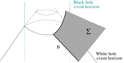
Figure 1: An example of non-smooth boundary $B=\partial\{\lambda>0\}$ in an initial data set $\Sigma$ of Kruskal spacetime with one dimension suppressed. The region outside the cylinder and the cone corresponds to one asymptotic region of the Kruskal spacetime. The initial data set $\Sigma$ intersects the bifurcation surface transversally. The shaded region corresponds to the intersection of $\Sigma$ with the asymptotic region, and is in fact a connected component of the subset $\{\lambda>0\}\subset\Sigma$. Its boundary is non-smooth at the points lying on the bifurcation surface.

We must therefore add some condition on $\partial\{\lambda>0\}$ in order to guarantee that this boundary does not intersects both a black and a white hole event horizon. In terms of the Killing vector, this requires that $\vec{Y}$ points only to one side of $\partial\{\lambda>0\}$. Proposition 1 suggests that the condition we need to impose is $Y^{i}D_{i}\lambda\big{|}_{\partial\{\lambda>0\}}\geq 0$ or $Y^{i}D_{i}\lambda\big{|}_{\partial\{\lambda>0\}}\leq 0$. This condition is in fact sufficient to show that $\partial\{\lambda>0\}$ is a smooth surface. More precisely

Proposition 3

Let $(\Sigma,g,K;N,\vec{Y},\tau)$ be a static KID and consider a connected component $E$ of $\{\lambda>0\}$. If $Y^{i}D_{i}\lambda\geq 0$ or $Y^{i}D_{i}\lambda\leq 0$ on each connected component of $B=\partial E$, then $B$ is at least $C^{1}$.

Proof. Both cases are similar so only the case $Y^{i}D_{i}\lambda\geq 0$ will be proven. If there are no fixed points, the result follows from Lemma 7. Let us therefore assume that there is at least one fixed point $p$. The idea of the proof is to show that $Y^{i}D_{i}\lambda\geq 0$ forces $b=0$ in (25) from which smoothness will follow. We argue by contradiction. Assume $b\neq 0$ in (25). In a neighbourhood of $p$, $D_{i}N\neq 0$ and we can use $x^{1}=N$ as a coordinate. Choosing coordinates $x^{A}=\{x,y\}$ on the slice $\{N=0\}$ and extending them as constants along $D_{i}N$, the metric $g$ takes the local form

$$ds^{2}=\frac{1}{Q^{2}}dN^{2}+g_{AB}(N,x^{C})dx^{A}dx^{B}.$$ (29)

Let us further choose $x^{A}$, so that $x^{A}(p)=0$, $g_{AB}|_{p}=\delta_{AB}$ and $dy|_{p}=\mbox{\boldmath$X$}$, where $X$ is the one-form appearing in (25). Expanding $Y_{i}$ in Taylor series we get $Y_{i}=s_{i}(x^{A})+W_{i}(x^{A})N+O(N^{2})$ with $s_{i}(x^{A}=0)=0$ since $p$ is a fixed point. Since $\frac{1}{N}(Y_{i}D_{j}N-Y_{i}D_{j}N)$ must have a finite limit at $p$ (it must in fact coincide with $f_{ij}|_{p}$, see (27)), it follows easily that $s_{A}=0$ on some neighbourhood of $p$. Restricting ourselves to such neighbourhood, we have $Y_{i}=\delta_{i}^{1}r(x^{A})+W_{i}(x^{A})N+O(N^{2})$ for some function $r(x^{A})$. At $p$, we have $\partial_{i}Y_{j}|_{p}=D_{i}Y_{j}|_{p}=f_{ij}|_{p}$ because $D_{(i}Y_{j)}=0$ from (2). Hence

$$\partial_{i}Y_{j}|_{p}=\left.\partial_{A}r\delta_{i}^{A}\delta_{j}^{1}+W_{j}\delta_{i}^{1}\right|_{p}=\frac{b}{Q_{0}}\left(\delta_{i}^{1}\delta_{j}^{2}-\delta_{j}^{1}\delta_{i}^{2}\right),$$

where (25) has been used in the second equality and $Q_{0}\equiv Q|_{p}$. Hence $\partial_{A}r|_{p}=-\frac{b}{Q_{0}}\delta_{A}^{2}$, $W_{A}|_{p}=\frac{b}{Q_{0}}\delta_{A}^{2}$ and $W_{1}|_{p}=0$. Consequently

$$Y_{1}=-\frac{b}{Q_{0}}y+O(2),\hskip 56.9055ptY_{A}=\delta_{A}^{2}\frac{b}{Q_{0}}N+O(2)$$

And then $\lambda=(1-\frac{b^{2}}{Q_{0}^{2}})N^{2}-b^{2}y^{2}+O(3)$. Recall that a connected component of $\{\lambda>0\}$ has either $N>0$ or $N<0$ everywhere. Let us choose $N>0$ for definiteness (the other case is similar). The boundary of this region has $N\geq 0$. Moreover, using $Q_{0}^{2}>b^{2}$ and the expression above for $\lambda$, it follows that, if $b\neq 0$, then $N$ vanishes on the boundary of $\{\lambda>0\}$ only when $y=0$. A direct calculation using the metric (29) gives now $Y^{i}D_{i}\lambda=-2bQ_{0}Ny+O(2)$. Thus, $Y^{i}D_{i}\lambda$ on the boundary changes sign with $y$ whenever $b\neq 0$. Consequently the hypothesis of the proposition demands $b=0$ and therefore $f_{ij}|_{p}=0$.

It only remains to show that in these circumstances, $B$ is $C^{1}$. We now have $D_{i}D_{j}\lambda|_{p}=2D_{i}ND_{j}N|_{p}$ and therefore $p$ is a degenerate critical point for $\lambda$. The Gromoll-Meyer splitting Lemma [15] implies that there exists coordinates $\{v,x^{\prime},y^{\prime}\}$ in a neighborhood of $p$ such that $p=\{v=0,x^{\prime}=0,y^{\prime}=0\}$ and $\lambda=v^{2}-q(x^{\prime},y^{\prime})$, for a smooth function $q$ satisfying $q(p)=0$, $D_{i}q|_{p}=0$ and $\mbox{Hess}(q)|_{p}=0$. But then, the boundary $B$ is locally defined by $v=\sqrt{q}$ (or with the minus sign, depending on which connected component is taken). The conditions on $q$ imply that $B$ is $C^{1}$ at $p$. $\hfill\Box$

Knowing that the surface is differentiable, our next aim is to show that, under suitable circumstances it is in fact a MOTS. This is the content of our last proposition in this Section.

Proposition 4

Let $(\Sigma,g,K;N,\vec{Y},\tau)$ be a static KID and consider a connected component $E$ of $\{\lambda>0\}$ with compact boundary $B=\partial E$. Assume

• $NY^{i}D_{i}\lambda|_{B}\geq 0$ if $B$ contains at least one fixed point.

• $NY^{i}m_{i}|_{B}\geq 0$ if $B$ contains no fixed point, where $\vec{m}$ is the unit normal pointing towards $E$.

Then $B$ is a MOTS with respect to the direction pointing towards $E$.

Remark. If the inequalities in (i) and (ii) are reversed, then $B$ is a MOTS with respect to the unit normal pointing outside of $E$.

Proof. Consider first the case when $B$ has at least one fixed point. Since $N$ is nowhere zero on $E$, it must be either non-negative or non-positive everywhere on $\partial E$. The hypothesis $NY^{i}D_{i}\lambda|_{B}\geq 0$ then implies either $Y^{i}D_{i}\lambda|_{B}\geq 0$ or $Y^{i}D_{i}\lambda|_{B}\leq 0$ and Proposition 3 shows that $B$ is a differentiable surface. Let $\vec{m}$ be the unit normal pointing towards $E$ and $p$ the corresponding mean curvature. Being $B$ also compact by hypothesis, it only remains to show that $p+\gamma^{AB}K_{AB}=0$.

Let us start by proving that $\vec{Y}$ is everywhere orthogonal to $B$. At the fixed points, this is trivial as $\vec{Y}=0$. For the open (possible empty) set $V$ of non-fixed points, we can construct the Killing development of a suitable neighbourhood and apply the Vishveshwara-Carter Lemma 6 to show that $V$ lies on a Killing Horizon and therefore $\vec{\xi}^{T}\big{|}_{B}=\vec{Y}^{T}\big{|}_{B}=0$. Moreover, Killing horizons necessarily have vanishing null expansion along to $\vec{\xi}$ and equations (1) and (14) imply

$$\theta_{\vec{\xi}}=Y_{\mu}p^{\mu}+NK_{AB}\gamma^{AB}|_{V}=0.$$ (30)

Now, Proposition 1 implies that $D_{i}\lambda\neq 0$ on $V$ so that $D_{i}\lambda|_{V}=Hm_{i}|_{V}$, for a positive function $H$. Using the fact that $\vec{Y}$ is parallel to $\vec{m}$, hypothesis (i) implies $\vec{Y}|_{V}=N\vec{m}|_{V}$. Dividing (30) by $N$ it follows that $V$ has vanishing outer null expansion with $\vec{m}$ pointing to the outer direction. The same conclusion holds by continuity on isolated fixed points. Open sets of fixed points are immediately covered by Proposition 2 because this set is then totally geodesic and $K_{AB}=0$, so that both null expansions vanish.

For the case that all points in $B$ are non-fixed, we know first of all that $B$ is smooth from Lemma 7, and hence $\vec{m}$ exists (this means in particular that hypothesis (ii) is well-defined). The same argument as before shows that $\vec{Y}$ is proportional to $\vec{m}$ and hypothesis (ii) implies $\vec{Y}=N\vec{m}$ everywhere, so (30) implies, as before, that the expansion along $\vec{m}$ vanishes. $\hfill\Box$

4 Main Results

In 2005 P. Miao [1] proved a uniqueness theorem which generalized the usual uniqueness theorem for static black holes by replacing the assumption of a black hole simply by the existence of a minimal surface. More precisely, Miao worked with KIDs which are (i) time-symmetric (which are defined by $K_{ij}=0,Y_{i}=0$), (ii) vacuum and (iii) asymptotically flat. The latter is defined as follows (recall that a function is said to be $O^{(k)}(r^{n})$, $k\in\mathbb{N}$ if $f(x^{i})=O(r^{n})$, $\partial_{j}f(x^{x^{i}})=O(r^{n-1})$ and so on for all derivatives up to an including the k-th ones).

Definition 10

A KID $(\Sigma,g,K;N,\vec{Y},\tau)$ is asymptotically flat if $\Sigma=K\cup\Sigma^{\infty}$, where $K$ is a compact set and $\Sigma^{\infty}=\underset{a}{\bigcup}\Sigma^{\infty}_{a}$ is a finite union with each $\Sigma^{\infty}_{a}$, called an “asymptotic end” being diffeomorphic to $\mathbb{R}^{3}\setminus\overline{B_{R_{a}}}$, where $B_{R_{a}}$ is an open ball of radius $R_{a}$. Moreover, in the Cartesian coordinates induced by the diffeomorphism, the following decay holds

$$N-A_{a}=O^{(2)}(1/r),\qquad g_{ij}-\delta_{ij} = O^{(2)}(1/r),$$

$$Y^{i}_{a}-C^{i}_{a}=O^{(2)}(1/r),\qquad\qquad K_{ij} = O^{(2)}(1/r^{2}).$$

where $A_{a}$ and $\{C^{i}_{a}\}_{i=1,2,3}$ are constants such that $A^{2}_{a}-\delta_{ij}C^{i}_{a}C^{j}_{a}>0$ for each $a$, and $r=\left(x^{i}x^{j}\delta_{ij}\right)^{1/2}$.

The condition on the constants $A_{a},C^{i}_{a}$ is imposed to ensure that the KID is timelike near infinity on each asymptotic end.

Miao’s theorem reads

Theorem 1 (Miao, 2005 [1])

Let $(\Sigma,h,K=0;N,\vec{Y}=0,\tau)$ be a time-symmetric, vacuum and asymptotically flat KID with a compact minimal surface (i.e. a surface of vanishing mean curvature) which bounds an open domain $W\subset\Sigma$.

Then $(\Sigma\setminus W,h)$ is isometric to $\left(\mathbb{R}\setminus B_{m/2}(0),g_{Schw}=\left(1+\frac{m}{2|x|}\right)^{4}\delta_{ij}\right)$ for some $m>0$.

Remark 1. The metric $g_{Schw}$ is the induced metric on the $\{t=0\}$ slice of the Schwarzschild spacetime with mass $m$, outside and including the horizon.

Remark 2. Actually, Miao’s theorem [1] deals with KIDs which have minimal boundaries. The formulation given above is in principle weaker but more suitable for our purposes.

One way of understanding the contents of this theorem is that a time-symmetric, vacuum and asymptotically flat Killing initial data set which contains a bounding minimal surface must in fact be a black hole and that the bounding minimal surface cannot penetrate into the exterior region defined as the connected component of $\{\lambda>0\}$ containing infinity. Thus, the minimal surface will be hidden inside the black hole and the usual uniqueness theorem for black holes implies that the slice must be Schwarzschild. The aim of the theorems below is to extend this result showing that bounding MOTSs cannot penetrate into the “exterior” region where the Killing vector is timelike. Our proof is strongly based on a powerful theorem recently proved by L. Andersson and J. Metzger [4], extending previous work by Schoen [16]. Let us first state this theorem.

4.1 Andersson & Metzger Theorem

The key object for the Andersson & Metzger theorem is that of weakly outer trapped region, defined as follows.

Definition 11

Let $(\Sigma,g,K)$ be an initial data set with an untrapped barrier surface $S_{b}=\partial{\mathfrak{D}}_{b}$. An open set $\Omega\subset{\mathfrak{D}}_{b}$ is called weakly outer trapped set if $\partial\Omega$ is a smooth embedded closed surface that is weakly outer trapped w.r.t. the normal pointing outside $\Omega$.

Definition 12

Let $(\Sigma,g,K)$ be an initial data set. The weakly outer trapped region, $T$, is defined as the union of all the weakly outer trapped sets.

Theorem 2 (Andersson & Metzger [4])

Let $(\Sigma,g,K)$ be a smooth, initial data set containing an untrapped barrier surface $S_{b}=\partial{\mathfrak{D}}_{b}$ with $\overline{{\mathfrak{D}}_{b}}$ complete. Let $T$ be the weakly outer trapped region. Then either $T=\emptyset$ or $\partial T$ is a smooth stable MOTS.

Remark. The definition of stable MOTS can be found in [17]. For the purposes of this paper, we only need the property that $\partial T$ is a MOTS.

4.2 Main Theorems

The idea of the proof of the theorems below is to assume the existence of a bounding MOTS $S$ in the exterior region, and use Andersson-Metzger theorem to pass to the outermost MOTS given by $\partial T$, which by construction must be on or outside $S$. Then, using stationarity and the null energy condition (NEC) we construct another MOTS strictly outside $\partial T$ therefore getting a contradiction.

Let us first recall the definition of null energy condition (NEC).

Definition 13

A Killing initial data set $(\Sigma,g,K;N,\vec{Y},\tau)$ satisfies the null energy condition (NEC) if for all $p\in\Sigma$ the tensor $G_{\mu\nu}\equiv\rho n_{\mu}n_{\nu}+J_{\mu}n_{\nu}+n_{\mu}J_{\nu}+\tau_{\mu\nu}|_{p}$ on $T_{p}\Sigma\times\mathbb{R}$ satisfies that $G_{\mu\nu}k^{\mu}k^{\nu}\geq 0$ for any null vector $\vec{k}\in T_{p}\Sigma\times\mathbb{R}$.

The first of our main theorems involves KIDs having an untrapped barrier surface with no further restriction. Staticity is not required for this result.

Theorem 3

Let $(\Sigma,g,K;N,\vec{Y},\tau)$ be a KID containing an untrapped barrier $S_{b}=\partial{\mathfrak{D}}_{b}$ and satisfying NEC. Assume that $\overline{{\mathfrak{D}}_{b}}$ is complete.

Then, there exists no bounding MOTS $S=\partial{\mathfrak{D}}$ with ${\mathfrak{D}}\subset{\mathfrak{D}}_{b}$ satisfying $\Sigma\setminus{\mathfrak{D}}\subset\{\lambda\geq 0\}$ provided $S\cap\{\lambda>0\}\neq\emptyset$.

Figure 2: Theorem 3 excludes the possibility that a MOTS like the one in the figure exists. The shaded area corresponds to the region where $\lambda$ is positive.

Remark 1. In short, the conditions of the theorem demands that the bounding MOTS is such that that Killing vector is causal everywhere on its exterior and timelike at least somewhere. When MOTS is replaced by the stronger condition of being a marginally trapped surface with one of the expansions non-zero somewhere, then this theorem can be proven by a simple argument based on the first variation of area [3]. In that case, the assumption of $S$ being bounding becomes unnecessary. It would be interesting to know if theorem 3 holds for arbitrary MOTSs, not necessarily bounding.

Remark 2. When the KID is asymptotically flat, the surface at constant $r$ on each one of the asymptotic ends is, for large enough $r$, outer untrapped. Thus, the domain ${\mathfrak{D}}_{b}$ can be taken as large as desired and in particular so that it contains any given MOTS $S$. In that case, the theorem asserts that there exists no bounding MOTS $S=\partial{\mathfrak{D}}$ in $\Sigma$ such that $\Sigma\setminus{\mathfrak{D}}\subset\{\lambda\geq 0\}$ and $S\cap\{\lambda>0\}\neq\emptyset$.

Two immediate, but useful corollaries follow.

Corollary 1

Assume that $\{\lambda>0\}=\Sigma$ on an asymptotically flat KID $(\Sigma,g,K;N,\vec{Y},\tau)$ satisfying NEC, then there exists no bounding MOTS in $\Sigma$.

Corollary 2

Let $(\Sigma,g,K)$ be an initial data set for Minkowski space, then there exists no bounding MOTS in $\Sigma$.

It is obvious that the second Corollary is a particular case of the first one because the $\partial_{t}$ in Minkowskian coordinates is strictly stationary everywhere, in particular on $\Sigma$. The non-existence result of a bounding MOTS in a Cauchy surface of Minkowski spacetime is however, well-known as this spacetime is obviously regular predictable (see [18] for definition) and then the proof of Proposition $9.2.8$ in [18] gives the result.

Proof. Under the conditions of the theorem, it is clear that ${\mathfrak{D}}$ belongs to the weakly outer trapped region $T$. Hence $\partial T\subset\{\lambda\geq 0\}$ with at least one point having $\lambda>0$.

Assume first that no point in $\partial T$ is fixed. Then $N\neq 0$ in some neighbourhood of $\partial T$ and we can construct the Killing development there. Since the KID satisfies NEC, so does the Killing development (the Einstein tensor is Lie constant along $\partial_{t}$). We can now consider the action of the local isometry group generated by the Killing vector $\vec{\xi}$, which is causal on $\partial T$. Let $\gamma$ be the group parameter and drag $\partial T$ with the local isometry a constant negative amount $\gamma_{0}$ of the group parameter ($\gamma_{0}$ can be chosen small enough so that the local group exists up to this value). Denote the image surface by $S^{\prime}$. Since $\vec{\xi}$ is future directed, $S^{\prime}$ lies strictly in the causal past of $\partial T$. Since geometric properties remain unchanged under the action of an isometry, $S^{\prime}$ is still a MOTS in the spacetime. Let $\vec{l}$ be the Lie dragging of $\vec{n}+\vec{m}$ onto $S^{\prime}$ and consider the null geodesics starting on $S^{\prime}$ and with tangent vector $\vec{l}$. This generates a null hypersurface which is smooth near enough $S^{\prime}$. Null hypersurfaces $\cal N$ ruled by a null vector $\vec{l}$ are endowed with a null expansion $\theta$ which has the property that any spacelike surface contained in $\cal N$ has null expansion with respect to $\vec{l}$ equal to $\theta$ (see e.g. [19]). Moreover $\theta$ obeys the Raychaudhuri equation: let $\beta$ be the affine parameter associated to $\vec{l}$ such that $\beta=0$ on $S^{\prime}$. Then

$$\frac{d\theta}{d\beta}=-\frac{1}{2}\theta^{2}-\sigma^{2}-G_{\mu\nu}l^{\mu}l^{\nu},$$

where $\sigma$ is the shear scalar of $\cal N$. Using NEC, all terms in the right hand side are non-positive. Since $\theta=0$ at $\beta=0$, it follows that $\theta$ is non-positive in the future of $S^{\prime}$ in $\cal N$. In general $\cal N$ will develop singularities in the future, however, the first singularity will occur for a finite value of $\beta$, which is independent of $\gamma_{0}$ (i.e. the amount we shifted $S$ to the past). It is therefore clear that by choosing $\gamma_{0}$ small enough, $S^{\prime\prime}\equiv\Sigma\cap\cal N$ will be a smooth surface (obviously lying in the future of $S^{\prime}$). By Raychaudhuri, this surface has non-positive outer expansion. Moreover, by construction $S^{\prime\prime}$ is also bounding for small enough $\gamma$ (because it is constructed by a continuous deformation of $\partial T$, which is bounding) and lies strictly in the exterior of $\partial T$ (because on at least one point of $S$ $\vec{\xi}$ is timelike). But this gives a contradiction since $S^{\prime\prime}$ must belong to $T$ by definition of $T$.

When $\partial T$ has fixed points, we cannot guarantee the existence of the Killing development on those points. However, letting $U\subset\partial T$ be the set of non-fixed points (which is obviously non-empty and open within $\partial T$), such development still exists in a neighbourhood of $U$. In this portion we can repeat the construction above and define $S^{\prime\prime}\subset\Sigma$. $N$ and $\vec{Y}$ being smooth and approaching zero at the fixed points, it follows easily that $S^{\prime\prime}$ and the set of fixed points $\partial T\setminus U$ will join smoothly and will therefore define a surface, which we still denote by $S^{\prime\prime}$. Moreover, this is still a bounding weakly outer trapped (it is still a continuous deformation of $S$) and therefore must be contained in $T$. But at least one point in $\partial T$ lies in $\{\lambda>0\}$, so that $U$ must be non-empty and $S^{\prime\prime}$ has at least one portion strictly outside $\partial T$, which gives the desired contradiction. $\hfill\square$

Notice that Corollary 1 together with Proposition 2 already imply the uniqueness part of Miao’s theorem. Indeed, Corollary 1 asserts that the existence of a bounding minimal surface in an asymptotically flat KID implies that $\partial\{\lambda>0\}$ is non-empty and compact, while Proposition 2 states that the set $\partial\{\lambda>0\}$ in such a time-symmetric KID is a totally geodesic surface in $\Sigma$ (in the time-symmetric case this was already known, see e.g. [20]). Thus, the usual uniqueness theorem for vacuum black holes implies that the exterior of this totally geodesic surface coincides with the $r>2m$ region of the $\{t=0\}$ slice in Schwarzschild coordinates. However, Miao’s result also states that the original minimal surface cannot penetrate into the exterior region $\{\lambda>0\}$. This last part is recovered (and extended) in our next theorem, where we show that bounding MOTSs cannot penetrate into the exterior $\{\lambda>0\}$ region in a static KID provided a suitable untrapped barrier surface exists (in particular in the asymptotically flat case).

Theorem 4

Let $(\Sigma,g,K;N,\vec{Y},\tau)$ be a static KID containing an untrapped barrier surface $S_{b}=\partial{\mathfrak{D}}_{b}$ and satisfying NEC. Assume that $\overline{{\mathfrak{D}}_{b}}$ is complete and $\Sigma\setminus{\mathfrak{D}}_{b}\subset\{\lambda>0\}$. Let $U$ be the connected component of $\{\lambda>0\}$ containing $\Sigma\setminus{\mathfrak{D}}_{b}$. Suppose that $\partial U$ is closed and

• $NY^{i}D_{i}\lambda|_{\partial U}\geq 0$ if $\partial U$ contains at least one fixed point.

• $NY^{i}m_{i}|_{\partial U}\geq 0$ if $\partial U$ contains no fixed point, where $\vec{m}$ is the unit normal pointing towards $U$.

Then, there exists no bounding MOTS $S=\partial{\mathfrak{D}}$, with ${\mathfrak{D}}\subset{\mathfrak{D}}_{b}$, intersecting $U$.

Figure 3: Theorem 4 forbids the existence of a bounding MOTS S like the one in the figure. The shaded area corresponds to the region where $\lambda$ is positive. $S_{b}$ is the untrapped barrier and the region it encloses is ${\mathfrak{D}}_{b}$.

Remark. In asymptotically flat KIDs the hypotheses of the theorem regarding the untrapped barrier and the compactness of $\partial U$ are automatically satisfied. Consequently, in this case no bounding MOTS intersecting $U$ can exist, provided (i) or (ii) hold.

Proof. First of all, we know from Proposition 4 that $\partial U$ is a MOTS. Assume there exists a bounding MOTS $S$ intersecting $U$. We know by definition of $T$ that both $\partial U$ and $S$ are contained in $T$. Therefore $\Sigma\setminus T\subset\overline{U}$ from which it follows that $\partial T\subset\overline{U}$ with at least one point in $U$. But then the same construction as in Theorem 3 gives a contradiction. $\hfill\square$

Clearly, this theorem recovers Miao’s result in the particular case of asymptotically flat time-symmetric vacuum KIDs containing a bounding minimal surface. Notice that when all points in $\partial U$ are fixed points $Y^{i}D_{i}\lambda\big{|}_{\partial U}$ is identically zero.

We finish this work remarking that the same effort used to prove the previous results leads to the following Corollary.

Corollary 3

Theorems 3 and 4, and Corollaries 1 and 2 also hold if “bounding MOTS” is replaced by bounding weakly outer trapped surface.

Proof. A bounding weakly outer trapped surface $S$ is included in the weakly outer trapped region $T$, so the same proof as before applies. $\hfill\square$

References

- [1] P. Miao, “A remark on boundary effects in static vacuum initial data sets”, Class. Quantum Grav. 22, L53-L59 (2005).
- [2] G. Bunting, A.K.M. Masood-ul-Alam, “Nonexistence of multiple black holes in asymptotically euclidean static vacuum space-time”, Gen. Rel. Grav. 19, 147-154 (1987).
- [3] M. Mars, J.M.M. Senovilla, “Trapped surfaces and symmetries”, Class. Quantum Grav. 20, L293-L300 (2003).
- [4] L. Andersson, J. Metzger, “The area of horizons and the trapped region”, arXiv:0708.4252.
- [5] G. Huisken, T. Ilmanen, “The inverse mean curvature flow and the Riemannian Penrose inequality”, J. Diff. Geom. 59, 353-437 (2001).
- [6] R. Beig, P.T. Chruściel, “Killing initial data”, Class. Quantum Grav. 14, A83-A92 (1997).
- [7] B. Coll, “On the evolution equations for Killing fields”, J. Math. Phys. 18, 1918-1922 (1977).
- [8] L.P. Eisenhart, “Riemannian Geometry”, Princeton Univ. Press, Princeton (1966).
- [9] W. Israel, “Differential Forms in General Relativity”, Comm. of the Dublin Inst. for Adv. Studies, series A, 19 (1970).
- [10] M. Mars, “A spacetime characterization of the Kerr metric”, Class. Quantum Grav. 16, 2507-2523 (1999).
- [11] P.T. Chruściel, “The classification of static vacuum space-times containing an asymptotically flat spacelike hypersurface with compact interior”, Class. Quantum Grav. 16, 661-687 (1999).
- [12] C.V. Vishveshwara, “Generalization of the ’Schwarzschild surface’ to arbitrary static and stationary metrics”, J. Math. Phys. 9, 1319-1322 (1968). B. Carter, “Killing horizons and orthogonally transitive groups in space-time, J. Math. Phys. 10, 70-81 (1969).
- [13] M. Heusler, “Black Hole Uniqueness Theorems”, Cambridge Lecture Notes in Physics 6 (Cambridge University Press, Cambridge, 1996).
- [14] R.H. Boyer, “Geodesic Killing orbits and bifurcate Killing horizons”, Proc. Roy. Soc. A. 311, 245-253 (1969).
- [15] D. Gromoll, W. Meyer, “On differentiable functions with isolated critical points”, Topology 8, 361-369 (1969).
- [16] R. Schoen, Talk given at the Miami Waves conference (Jan. 2004).
- [17] L. Andersson, M. Mars, W. Simon, “Stability of marginally outer trapped surfaces and existence of marginally outer trapped tubes”, arXiv:0704.2889.
- [18] S.W. Hawking, G.F.R. Ellis, “The large scale structure of space-time”, Cambridge monographs on mathematical physics, (Cambridge University Press, 1973).
- [19] G.J. Galloway, “Maximum principles for null hypersurfaces and null splitting theorems”, Ann. Poincaré Phys. Theory 1, 543-567 (2000).
- [20] J. Corvino, “Scalar Curvature Deformation and a Gluing Construction for the Einstein Constraint Equations”, Commun. Math. Phys. 214, 137-189 (2000).