A further look at particle annihilation in dark matter caustics

Abstract

Dark matter caustics are small scale, high density structures believed to exist in galaxies like ours. If the dark matter consists of Weakly Interacting Massive Particles, these caustics may be detected by means of the gamma rays produced by dark matter particle annihilation. We discuss particle annihilation in outer and inner caustics and provide sky maps of the expected gamma ray distribution.

I Introduction

A consequence of the presence of cold dark matter in galactic halos is the formation of caustics. Caustics are regions of infinite density in the limit where the dark matter particles have zero velocity dispersion. The leading dark matter candidates, namely axions and Weakly Interacting Massive Particles(WIMPs), have very small primordial velocity dispersions ($\sim 0.03$ cm/s for a 100 GeV WIMP, $\sim 10^{-6}$ cm/s for a 10 $\mu$eV axion ps_crs ) and may be expected to form caustics with large density enhancements. If the dark matter is made up of WIMPs, the particles can annihilate producing gamma rays. It may be possible to detect this gamma ray flux by means of future experiments such as GLAST glast . Caustics may possibly be revealed by this technique.

Caustics form because cold dark matter particles occupy a thin, three dimensional hypersurface in phase space ps_crs ; caustic_papers . There are two kinds of caustics in galactic halos: outer and inner ps_crs . The outer caustics are topological spheres surrounding galaxies. The inner caustics have a more complicated geometry which depends on the details of the dark matter angular momentum distribution ns2 . When the angular momentum distribution is dominated by a net rotational term, the inner caustics have the appearance of rings ps_crs ; ns2 . Observational evidence for caustic rings was found by analyzing the rotation curves of external galaxies ks and the rotation curve of the Milky Way iras . A triangular feature seen in the Infrared Astronomical Satellite (IRAS) map of the Milky Way is also suggestive of the presence of a nearby inner caustic ring iras . Recently os , possible evidence was found for a caustic ring in the galaxy cluster Cl0024+1654. In this article, we discuss dark matter annihilation in caustic spheres and caustic rings and present simulated gamma ray sky maps.

The existence of dark matter caustics is sometimes disputed on the basis of large scale cosmological simulations. However, current simulations use particles with mass of order $\sim 10^{6}M_{\odot}$. Such massive particles have spurious collisions which destroy fine details in the dark matter phase space hypersurface. Thus the absence of caustics in most large scale simulations is probably due to the finite resolution of these simulations and the large particle masses involved. Note that discrete flows and caustics are observed in $N$-body simulations when special care is taken. The simulations of Stiff and Widrow Sti , which increase the resolution in the relevant regions of phase space, do show discrete flows. More recently, Vogelsberger et al. Voge employed a new technique to study small scale structures such as caustics. Further progress in numerical techniques may enable the study of caustic properties in galactic halos using $N$-body simulations.

In cold dark matter cosmology, galactic halos form through a process of “hierarchical clustering”. Small halos form first. Larger halos, such as that of the Milky Way, are the outcome of past mergers, the accretion of smaller halos of various sizes, and the accretion of unclustered dark matter. This general scenario must surely be correct without, however, telling us anything precise. The critical issue for the existence of a caustic is the velocity dispersion of the flow that would form it. To be specific, consider the flow of dark matter that the Milky Way halo is accreting today. If the dark matter in this flow has not clustered on any small scales yet, its velocity dispersion has the primordial value mentioned earlier, of order 0.03 cm/s for a 100 GeV WIMP. If it has clustered already, its effective velocity dispersion is the velocity dispersion of the structure it has become part of. The largest structures for which we have evidence of recent accretion are small sattelites, such as the Sagittarius dwarf, with velocity dispersion of order 10 km/s. So one may conservatively assume that the flow of WIMP dark matter accreting onto the Galaxy today has variable velocity dispersion between 0.03 cm/s and 10 km/s.

Dark matter caustics are generically surfaces on one side of which the density diverges, in the limit of zero velocity dispersion, as

$$d(x)={A\over\sqrt{x}}$$ (1)

where $x$ is the distance to the surface and $A$ is a constant called the “fold coefficient”. For finite velocity dispersion $\delta v$, the dark matter caustics in a galactic halo are smoothed over a distance

$$\delta x\sim{\delta v\over v}R$$ (2)

where $v$ is the flow velocity (of order 300 km/s) and $R$ is the overall size of the halo (of order 300 kpc). The velocity dispersion cuts off the divergence of the density at the caustic, i.e. the ${1\over\sqrt{x}}$ behaviour stops for $x<\delta x$. For the above range of velocity dispersion, $\delta x$ ranges from $10^{15}$ cm to 10 kpc. Since outer caustics have size of order hundreds of kpc, they are not erased by the expected velocity dispersion. Inner caustics which have size of order 10 kpc are smoothed out only when the flow is entirely composed of sattelites with velocity dispersion of order 10 km/s.

As was mentioned, evidence for caustic rings of dark matter in the Milky Way was found in the existence and distribution of sharp rises in the Galactic rotation curve and the presence of a triangular feature in the IRAS map of the Galactic plane iras . This evidence implies an upper limit on the velocity dispersion of order 50 m/s, or an upper limit on the smoothing scale $\delta x$ of order $10^{-4}~{}R\sim 30$ pc.

The WIMP annihilation rate per unit surface of caustic is proportional to the integral

$$\int dx~{}d(x)^{2}\simeq\int_{\delta x}^{R}{A^{2}\over x}=A^{2}\ln\left({R\over\delta x}\right)~{}~{}~{}\ .$$ (3)

This equation shows that caustics enhance the annihilation signal only by a logarithmic factor detecting which varies from $\sim 3$ to 20, depending on the velocity dispersion.

In this article, we limit ourselves to the simple cases of a spherically symmetric outer caustic and an axially symmetric inner caustic ring. Our symmetry assumptions are made solely for the purpose of computational ease. In previous work ns2 , we verified that caustics are stable under perturbations, in particular perturbations that break any assumed symmetry. Moreover, the symmetry assumptions are consistent with the observational evidence mentioned earlier.

Previous work on the possibility of detecting dark matter caustics by indirect means include detecting ; pieri ; an ; mss . Caustics and cold flows are also relevant to WIMP and axion direct detection experiments direct .

The number of photons received by a detector per unit area, per unit time, per unit solid angle and per unit energy due to WIMP annihilation is given by the expressionpieri ; gondolo

$$\frac{d\Phi}{d\Omega dE_{\gamma}}(E_{\gamma},l,b)=\frac{dS}{dE_{\gamma}}(E_{\gamma})\times\frac{E(l,b)}{4\pi}.$$ (4)

The term $dS/dE_{\gamma}$ depends only on the particle physics:

$$\frac{dS}{dE_{\gamma}}(E_{\gamma})=\frac{<\sigma_{a}v>}{2m^{2}_{\chi}}\sum_{i}b_{i}\;\frac{dN_{\gamma,i}}{dE_{\gamma}}(E_{\gamma}).$$ (5)

$<\sigma_{a}v>$ is the WIMP annihilation cross section times the relative velocity averaged over the momentum distribution of the WIMPs, $m_{\chi}$ is the WIMP mass, $dN_{\gamma,i}/dE_{\gamma}$ is the number of photons produced per annihilation per unit energy $E_{\gamma}$ in the annihilation channel $i$, and $b_{i}$ is the branching fraction of channel $i$.

The term $E(l,b)$ is called the emission measure and depends solely on the dark matter distribution.

$$E(l,b)=\int_{los}dx\;d^{2}(x)$$ (6)

where $x(l,b)$ is the distance measured along the line of sight($los$) in the direction of the galactic co-ordinates $(l,b)$, and $d$ is the dark matter density. Since all detectors have a finite resolution, the emission measure is often expressed in terms of $<E>$, which represents an average over the resolution of the detector. In this article, we limit ourselves to computing $E(l,b)$.

As an example, let us compute the emission measure due to a smooth isotropic halo with the density profile

$$d(r)=d(r_{0})\,\frac{r_{0}^{2}+a^{2}}{r^{2}+a^{2}}.$$ (7)

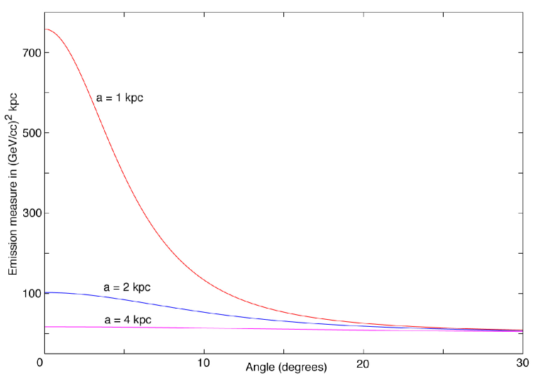
Figure 1: Emission measure due to a smooth halo with the density profile of Eq. 7 with $a$ = 1 kpc, 2 kpc and 4 kpc. $r_{0}=8.5$ kpc and $d_{0}=0.3$ GeV/cm³.

Consider an observer at a distance $r_{0}$ from the center of the halo, and a line of sight making an angle $\psi$ with the line joining the observer with the center (we choose $\psi=0$ to be the direction of the halo center). $a$ is the core radius and keeps the density finite. We choose $d=0.3$ GeV/cm³ when $r=r_{0}=8.5$ kpc. The emission measure $E$ is plotted as a function of angle $\psi$ in Fig. 1, for the cases $a=1,2$ and 4 kpc.

II Outer caustics

Outer caustics are topological spheres. They are fold catastrophes with the universal density profile

$$d(r)=\frac{A}{\sqrt{R-r}}\;\Theta(R-r)$$ (8)

where $d(r)$ is the dark matter density, $r$ is the distance from the center of the sphere, measured along the radial direction, $R$ is the radius of the sphere, $A$ is a constant for the particular caustic, and $\Theta$ is the unit step function. For the self-similar infall model ss1 ; ss2 ; ss3 of the Milky Way halo, the radii of the first $n=1,2,3,\cdots$ outer caustics $R_{n}\simeq\{440,260,190,150,120,\cdots\}$ kpc ss3 and the corresponding values of $A_{n}$ $\simeq\{8,9,10,10,11,\cdots\}\times 10^{-4}M_{\odot}/\textrm{pc}^{5/2}$ ss3 . We will assume a thickness $\delta R$ for the caustic sphere, which sets a density cutoff equal to $A/\sqrt{\delta R}$.

II.1 Observer outside the caustic sphere

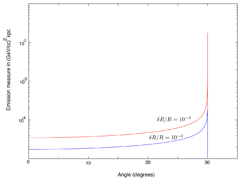
Figure 2: Emission measure from a spherical outer caustic(observer outside the sphere) for $\delta R/R=10^{-8}$ and $\delta R/R=10^{-4}$. $r_{0}/R=2$. The constant $A$ was chosen to be $0.97\times 10^{-3}\frac{\textrm{GeV}}{\textrm{cc}}\sqrt{\textrm{kpc}}=8.1\times 10^{-4}\frac{\textrm{M}_{\odot}}{\textrm{pc}^{5/2}}$.

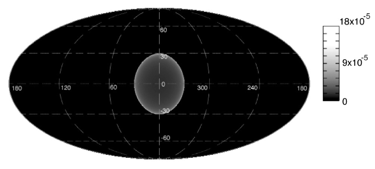
Figure 3: Simulated skymap of the emission measure from a spherical outer caustic, with the observer being located outside the sphere. $r_{0}/R=2,\delta R/R=10^{-4},A=0.97\times 10^{-3}\frac{\textrm{GeV}}{\textrm{cc}}\sqrt{\textrm{kpc}}$. The scale shows $E$ / (GeV/cc)² kpc.

Consider a spherical outer caustic of radius $R$ and thickness $\delta R$. Let an observer be located at a distance $r_{0}$ from the center of the sphere $(r_{0}>R)$. Consider a line of sight passing through the sphere making an angle $\psi$ with the line joining the observer with the center of the sphere($\psi=0$ is the direction of the center). The emission measure $E$ is plotted in Fig. 2 for $r_{0}/R=2$, for the two cases $\delta R/R=10^{-8}$ and $\delta R/R=10^{-4}$. The maximum value of $E\approx 1.87A^{2}\sqrt{R/\delta R}$ occurs when the line of sight is tangent to the sphere. Fig. 3 shows a simulated sky map.

II.2 Observer inside the caustic sphere

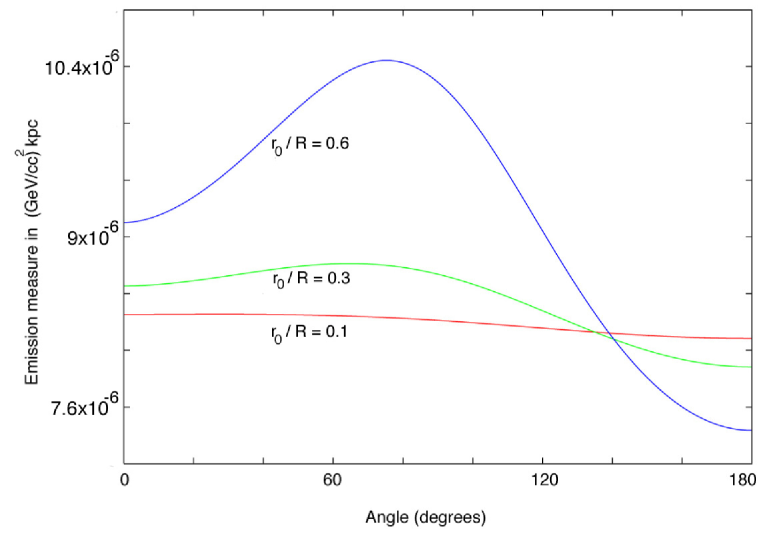
Figure 4: Emission measure from a spherical outer caustic (observer inside the sphere). Shown are three cases: $r_{0}/R=0.1,0.3,0.6$. The constant $A$ was chosen to be $0.97\times 10^{-3}\frac{\textrm{GeV}}{\textrm{cc}}\sqrt{\textrm{kpc}}$ and $\delta R/R=10^{-4}$.

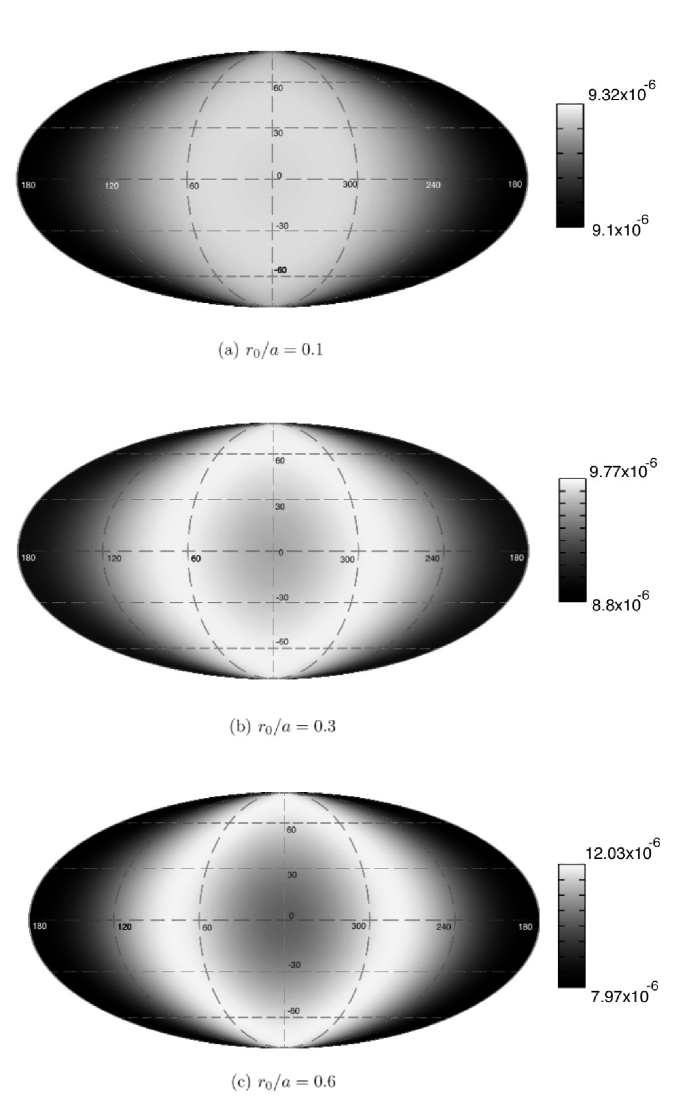
Figure 5: Simulated sky maps of the emission measure due to a spherical outer caustic, with the observer located within the sphere. Shown are the three cases: $(a)r_{0}/R=0.1,(b)r_{0}/R=0.3$ and $(c)r_{0}/R=0.6$. $A$ was chosen to be $0.97\times 10^{-3}\frac{\textrm{GeV}}{\textrm{cc}}\sqrt{\textrm{kpc}}$. $\delta R/R=10^{-4}$. The scale shows $E$ / (GeV/cc)² kpc.

Let us now consider the case where the observer is within the caustic sphere. We once again assume a sphere of radius $R$ and thickness $\delta R$. The observer is located at a distance $r_{0}$ from the center($r_{0}<R$). As before, $\psi$ is the angle made by the line of sight with the line joining the observer with the center ($\psi=0$ gives the direction of the center). Fig. 4 shows the emission measure plotted as a function of angle $\psi$ for the three cases $r_{0}/R=0.1,0.3$ and $0.6$. Figs. 5 (a),(b),(c) show simulated skymaps.

In both cases, the emission measure for the first few outer caustics of a halo like the Milky Way is quite small compared to that obtained from the smooth halo of Eq. 7, for $\delta R/R>10^{-10}$. However, $E$ would be larger for caustics of smaller radii and could possibly make a significant contribution to the total flux mss .

III Inner caustics

The inner caustics are made up of sections of the higher order catastrophes. As mentioned in the Introduction, the inner caustics resemble rings when the dark matter angular momentum distribution is dominated by a net rotational term. Here, we assume that this is the case. A caustic ring is a closed tube whose cross section has three cusps. Consider a caustic ring of radius $a$, horizontal extent $p$ and vertical extent $q$. See ps_crs for details. We choose cylindrical co-ordinates $(z,\rho=\sqrt{x^{2}+y^{2}})$. Let us define the two dimensionless variables $X=(\rho-a)/p$ and $Z=z/q$. For simplicity, we assume axial symmetry about the $Z$ axis and reflection symmetry about the $Z=0$ plane. With these assumptions, we can obtain an analytic expression for the density $d$ close to a caustic ring, in the limit $p,q\ll a$. For the special case of $Z=0$, the dark matter density is given by an

$$d(X,0)=\frac{fv^{2}_{rot}}{4\pi G}\left\{\begin{array}[]{lll}\frac{1}{1-X}&\mbox{ when $X\leq 0$ }\\ \frac{1}{1-X}\left(1+\frac{1}{\sqrt{X}}\right)&\mbox{ when $0\leq X\leq 1$ }\\ \frac{1}{X-1}&\mbox{ when $X\geq 1$. }\end{array}\right.$$ (9)

$f$ is a constant for the particular caustic ring. For the self-similar infall model of the Milky Way halo ss2 ; ss3 , $f_{n}\approx\{0.11,0.046,0.029,0.021,0.017,...\}$ for the first few $n=1,2,3,...$ dark matter flows. For the more general case of non-zero Z, the density $d(Z,X^{2})$ takes the form an :

$$d(X,Z^{2})=\frac{fv^{2}_{rot}}{4\pi G}\;\sum_{i}\frac{1}{2\left|1-X+2\,T^{2}_{i}-3T_{i}\right|}$$ (10)

where $T_{i}$ are the real roots of the quartic equation

$$T^{4}-2\,T^{3}+(1-X)\,T^{2}-\frac{27}{64}Z^{2}=0.$$ (11)

Note that the assumption of reflection symmetry about the $Z=0$ plane implies that the dark matter density is a function of $Z^{2}$. See Appendix A for a derivation of Eqs. 9 - 11

III.1 Observer outside the caustic ring tube

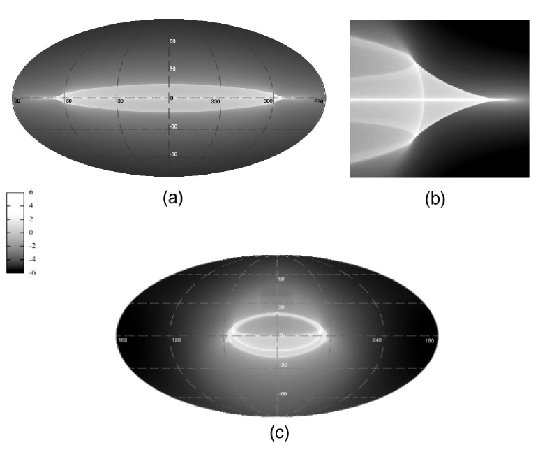
Figure 6: Simulated sky maps of the emission measure from an inner caustic ring, with the observer located outside the ring. $f$ was chosen to be 0.02 and $p/q=1$. (a) shows a caustic ring aligned with the galactic plane, with $a/r_{0}=15/17$ and $p/a=1/15$. The tricusp cross section of the ring is shown in detail in (b). (c) shows a caustic ring inclined to the galactic plane. The scale shows $\log_{e}$[$E$/(GeV/cc)² kpc].

Consider an observer located at a distance $r_{0}$ from the center of a circular caustic ring with $p=q$ and $r_{0}>a+p$. Fig. 6 shows simulated skymaps of the emission measure. The caustic ring is aligned with the galactic plane in (a) and inclined to the plane in (c). The emission measure is largest when the line of sight is tangent to the ring. The tricusp shape of the cross section is clearly visible in (b).

III.2 Observer inside the caustic ring tube

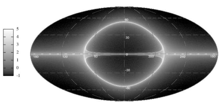
Figure 7: Simulated sky map of the emission measure from an inner caustic ring, with the observer located within the tricusp tube. The ring is aligned with the galactic plane. $p/q=1$ and $f=0.02$. The emission measure is largest when the lines of sight pass close to the cusps, resulting in the bright ring seen in the figure. The scale shows $\log_{e}$[E/(GeV/cc)² kpc].

Let us now consider the case where the observer is located within the tricusp shaped tube of a circular caustic ring. The observer is in the plane of the ring at a distance $r_{0}$ from the center with $a<r_{0}<a+p$. We also set $p=q$. Fig. 7 shows a simulated skymap of the emission measure. The bright ring and the line at $b=0$ occur when the lines of sight pass close to the cusps.

We see that for the inner caustics, the emission measure can be much larger than that obtained from a smooth halo (except near the center of the halo). For a comparison of the annihilation flux with the measured gamma ray background, we refer the reader to an .

IV Conclusion

We have discussed dark matter annihilation in outer and inner caustics and provided simulated skymaps of the emission measure. In Section II, we considered spherical outer caustics. When the observer is located outside the sphere, the emission measure $E$ is largest when the line of sight is tangent to the sphere, falling off rapidly to zero thereafter (Figs 2,3). When the observer is within the sphere, the emission measure only changes gradually with the angle $\psi$ (Figs. 4,5).

In Section III, we considered circular, symmetric tricusp ring caustics. When the observer is outside the caustic ring, the emission measure is largest when the line of sight is tangent to the ring. Looking tangentially, one may hope to identify the tricusp cross section of the ring[Fig. 6(b)]. When the observer is within the tricusp, the emission measure is largest when the lines of sight pass close to the cusps, resulting in the bright ring seen in Fig. 7. We find that for inner caustics, $E$ can be significantly larger than that produced by a smooth halo, especially in directions away from the halo center.

Appendix A Dark matter density near an axially symmetric caustic ring.

Consider a single cold flow of dark matter particles falling in and out of the halo, forming a caustic. Let us consider cylindrical co-ordinates $(\rho,z)$ where $\rho=\sqrt{x^{2}+y^{2}}$. For simplicity, we assume axial symmetry about the $z$ axis and reflection symmetry about the $z=0$ plane. Let $\rho=a$ be the caustic ring radius, defined as the point of closest approach of the particles in the $z=0$ plane (the particles with the most angular momentum are in this plane). Consider a reference sphere such that each particle in the flow passes through the sphere once. We can then assign to each particle in the flow, a two parameter label $(\alpha,\tau)$ which serves to identify the particle. We choose $\alpha=\pi/2-\theta$ where $\theta$ is the polar angle of the particle at the time it crossed the reference sphere. $\tau=0$ is the time when the particles just above the $z=0$ plane cross this plane. See ps_crs for details. We may expand $\rho$ and $z$ in a Taylor series ps_crs ,

$$\rho(\alpha,\tau)-a = \frac{1}{2}u\left(\tau-\tau_{0}\right)^{2}-\frac{1}{2}s\alpha^{2}$$

$$z(\alpha,\tau) = b\,\alpha\,\tau$$ (12)

where $b,u,s,\tau_{0}$ and the ring radius $a$ are constants for a given flow. In terms of these constants, we can express the horizontal ($p$) and vertical ($q$) extents of the tricusp:

$$p = \frac{1}{2}u{\tau_{0}}^{2}$$

$$q = \frac{\sqrt{27}}{4}\,\frac{bp}{\sqrt{us}}.$$ (13)

Let us define the dimensionless variables $X$ and $Z$

$$X = \frac{\rho-a}{p}$$

$$Z = \frac{z}{q}.$$ (14)

Using Eq. 13 and Eq. 14, we may express Eq. 12 in terms of $X$ and $Z$

$$X = \left(T-1\right)^{2}-\frac{27}{64}\left(\frac{b\tau_{0}\alpha}{q}\right)^{2}$$

$$Z = \frac{b\tau_{0}\alpha}{q}\,T$$ (15)

where $T=\tau/\tau_{0}$. The density at points close to the caustic is given by ps_crs

$$d(X,Z^{2})=\frac{1}{\rho}\sum\frac{dM}{d\Omega dt}\frac{\cos\alpha}{|D_{2}|}$$ (16)

where $|D_{2}|$ is the absolute value of the two dimensional Jacobian determinant $\left|\partial(x,y)/\partial(\alpha,\tau)\right|$

$$\left|D_{2}\right|=\left|2bp\left[1-X+2T^{2}-3T\right]\right|$$ (17)

and the sum is over the individual dark matter flows that exist at that point. We use the self-similar infall halo model with angular momentum ss2 to estimate the mass infall rate

$$\frac{dM}{d\Omega dt}=f\,v\,\frac{v^{2}_{rot}}{4\pi G}.$$ (18)

$f$ is a parameter that characterizes the density of the flow , $v$ is the speed of the particles forming the caustic, and $v_{rot}$ is the rotation velocity of the halo.

A.1 Case 1: $Z=0$

Let us first consider the simple case of points in the $Z=0$ plane. When $Z=0$, there are two flows at each point when $X>1$, four flows at each point for $0\leq X\leq 1$ and two when $X<0$.

A.1.1 $X>1$

When $X>1$, we have two possible solutions: $T=1\pm\sqrt{X}$ corresponding to the two flows that exist at each point. Using Eq.16, 17 and 18, and approximating $\cos\alpha\approx 1$ and $a\gg p$ we find the dark matter density at points close to the caustic

$$d(X,0;X>1)=\frac{fv^{2}_{rot}}{4\pi G}\,\frac{v}{b}\,\frac{1}{ap}\,\frac{1}{X-1}.$$ (19)

A.1.2 $0\leq X\leq 1$

In this range, we have four possible solutions: $T=0,0,1\pm\sqrt{X}$. Summing over the four solutions, we find

$$d(X,0;0\leq X\leq 1)=\frac{fv^{2}_{rot}}{4\pi G}\,\frac{v}{b}\,\frac{1}{ap}\,\frac{1}{1-X}\left(1+\frac{1}{\sqrt{X}}\right).$$ (20)

A.1.3 $X<0$

For $X<0$, we once again have two solutions $T=0,0$. The dark matter density is:

$$d(X,0;X<0)=\frac{fv^{2}_{rot}}{4\pi G}\,\frac{v}{b}\,\frac{1}{ap}\,\frac{1}{1-X}.$$ (21)

A.2 Case 2: $Z\neq 0$

We now consider the general case of computing the dark matter density at points outside the $Z=0$ plane. For $Z\neq 0$, neither $\alpha$ nor $T$ can be zero, so we may express $\alpha$ in terms of $T$ in Eq. 15, to obtain a quartic equation for $T$:

$$T^{4}-2T^{3}+(1-X)T^{2}-\frac{27}{64}Z^{2}=0.$$ (22)

The dark matter density is given by

$$d(X,Z^{2})=\frac{fv^{2}_{rot}}{4\pi G}\,\frac{v}{b}\;\sum_{i}\frac{1}{2\left|1-X+2\,T^{2}_{i}-3T_{i}\right|}$$ (23)

where $T_{i}$ are the real roots of Eq. 22. The number of real roots is given by the sign of the discriminant

$$\beta=-\frac{27Z^{2}}{4}\,\left[\left(\frac{27Z^{2}}{16}\right)^{2}+\frac{27Z^{2}}{16}\left(2X^{2}+5X-\frac{1}{4}\right)+X(X-1)^{3}\right].$$ (24)

There are four real roots if $\beta>0$ and two if $\beta<0$.

To solve Eq. 22, let us make the substitution $T_{1}=T-1/2$, thereby eliminating the cubic term in Eq. 22:

$${T_{1}}^{4}-\left(X+\frac{1}{2}\right){T_{1}}^{2}-XT_{1}-\Gamma=0$$ (25)

where $\Gamma=\frac{27}{64}Z^{2}+\frac{X}{4}-\frac{1}{16}$. We may solve Eq. 25 by expressing it as the product of two quadratics:

$$\left({T_{1}}^{2}+CT_{1}+D\right)\left({T_{1}}^{2}-CT_{1}-\frac{\Gamma}{D}\right)=0.$$ (26)

$C^{2}$ solves the cubic

$$\left[C^{2}\right]^{3}-2(X+\frac{1}{2})\left[C^{2}\right]^{2}+\left[\left(X+\frac{1}{2}\right)^{2}+4\Gamma\right]C^{2}-X^{2}=0$$ (27)

and

$$D=\frac{1}{2}\left[C^{2}-(X+\frac{1}{2})+\frac{X}{C}\right].$$ (28)

Let us define the two variables $M$ and $N$

$$M = \left(\frac{X-1}{3}\right)^{2}-\frac{9Z^{2}}{16}$$

$$N = -\left(\frac{X-1}{3}\right)^{3}-\frac{9Z^{2}}{16}\left(X+\frac{1}{2}\right).$$ (29)

$C^{2}$ has one real root

$$C^{2}=\frac{2}{3}\left(X+\frac{1}{2}\right)+\left(N+\sqrt{N^{2}-M^{3}}\right)^{1/3}+\left(N-\sqrt{N^{2}-M^{3}}\right)^{1/3}$$ (30)

if $N^{2}>M^{3}$ and three real roots

$$C^{2}=\frac{2}{3}\left(X+\frac{1}{2}\right)+2\sqrt{M}\,\cos\left(\frac{2n\pi}{3}+\frac{1}{3}\cos^{-1}\frac{N}{M\sqrt{M}}\right)$$ (31)

for $n=0,1,2$ if $N^{2}<M^{3}$. $D$ may be obtained using any of the values of $C$. The desired solution of the quartic Eq. 22 is then

$$T=\left\{\begin{array}[]{ll}\frac{1-C}{2}\pm\sqrt{\left(\frac{C}{2}\right)^{2}-D}\\ \frac{1+C}{2}\pm\sqrt{\left(\frac{C}{2}\right)^{2}+\frac{\Gamma}{D}}\end{array}.\right.$$ (34)

Once the real roots $T_{i}$ are known, Eq. 23 and $v\approx b$ may be used to obtain the dark matter density.

References

- (1) P. Sikivie, Phys. Rev. D 60, 063501 (1999)
- (2) M. Kachelriess, P.D. Serpico, arXiv: hep-ph/0707.0209v1 (2007); L. Wai, GLAST LAT Collaboration, arXiv: astro-ph/0701885v1 (2007)
- (3) V.I. Arnold, S.F. Shandarin, Y.B. Zeldovich, Geophysical and Astrophysical Fluid Dynamics, 20, 111 (1982); S.F. Shandarin and Y.B. Zeldovich, Rev. Mod. Phys. 61, 185 (1989); P. Sikivie and J.R. Ipser, Phys. Lett. B 291, 288 (1992); A. Natarajan and P. Sikivie, Phys. Rev. D 72, 083513 (2005)
- (4) A. Natarajan and P. Sikivie, Phys. Rev. D 73, 023510 (2006)
- (5) W.H. Kinney and P. Sikivie, Phys. Rev. D 61, 087305 (2000)
- (6) P. Sikivie, Phys. Lett. B 567 1 (2003)
- (7) V. Onemli and P. Sikivie, arXiv: astro-ph/0710.4936v1 (2007)
- (8) D. Stiff and L.M. Widrow, Phys. Rev. Lett. 90, 211301 (2003)
- (9) M. Vogelsberger, S.D.M. White, A. Helmi and V. Springel, arXiv:0711.1105 [astro-ph].
- (10) C.J. Hogan, Phys. Rev. D 64, 063515 (2001); L. Bergström, J. Edsjo and C. Gunnarsson, Phys. Rev D, 63 083515 (2001); C. Charmousis, V. Onemli, Z. Qiu and P. Sikivie, Phys. Rev D67, 103502 (2003); R. Gavazzi, R. Mohayaee and B. Fort, Astron. & Astrophys., 445, 43 (2006); V. K. Onemli, Phys. Rev. D 74, 123010 (2006); R. Mohayaee and S.F. Shandarin, Mon. Not. R. Astron. Soc. 366, 1217 (2006);
- (11) L. Pieri and E. Branchini, J. Cosmol. Astropart. Phys. JCAP05(2005)007;
- (12) A. Natarajan, Phys. Rev. D 75, 123514 (2007)
- (13) R. Mohayaee, S. Shandarin and J. Silk, JCAP05(2007)015
- (14) G. Gelmini and P. Gondolo, Phys. Rev D 64, 023504 (2001); A.M. Green, Phys. Rev. D 63, 103003 (2001); J. D. Vergados, Phys. Rev. D 63, 063511 (2001); F.S. Ling, P. Sikivie and S. Wick, Phys. Rev. D 70, 123503 (2004); L.D. Duffy et al, Phys. Rev. D 74, 012006 (2006); C. Savage, K. Freese and P. Gondolo, Phys. Rev. D 74, 043531 (2006)
- (15) J. Hall and P. Gondolo, Phys. Rev. D74, 063511 (2006)
- (16) J.A. Filmore and P. Goldreich, Ap. J. 281, 1 (1984); E. Bertschinger, Ap. J. Suppl., 58, 39 (1985)
- (17) P. Sikivie, I.I. Tkachev and Y. Wang, Phys. Rev. Lett. 75, 2911 (1995); P. Sikivie, I.I. Tkachev and Y. Wang, Phys. Rev. D 56, 1863 (1997)
- (18) L.D. Duffy and P. Sikivie, in preparation.