Direct numerical simulations of the -mechanism
Abstract
Context. Hydrodynamical model of the -mechanism in a purely radiative case.
Aims. First, to determine the physical conditions propitious to -mechanism in a layer with a configurable conductivity hollow and second, to perform the (nonlinear) direct numerical simulations (DNS) from the most favourable setups.
Methods. A linear stability analysis applied to radial modes using a spectral solver and DNS thanks to a high-order finite difference code are compared.
Results. Changing the hollow properties (location and shape) lead to well-defined instability strips. For a given position in the layer, the amplitude and width of the hollow appear to be the key parameters to get unstable modes driven by -mechanism. The DNS achieved from these more auspicious configurations confirm the growth rates as well as structures of linearly unstable modes. The nonlinear saturation follows through intricate couplings between the excited fundamental mode and higher damped overtones.
Key Words.:
Hydrodynamics - Instabilities - Waves - Stars: oscillations - Methods: numerical1 Introduction
Since the beginning of the studies concerning Cepheids, it is well known that convection occurs in Cepheids’ envelopes, and thus changes pulsation properties (e.g. the reviews of Gautschy & Saio 1996; Buchler 1997). The coldest ones, which are located next to the red edge of the instability strip, have the more extended surface convective zones. However, during many years Cepheids’ oscillations models have used the so-called “frozen-in convection” approximation which claims that convective flux perturbations are negligible (Baker & Kippenhahn 1962). Such kind of models well predict the blue edge of the instability strip but fail to explain the red edge as in this case, the strong existing couplings between the convection and the oscillations are not taken into account. This discrepancy becomes obvious with the accumulation of accurate observations which show a narrower instability strip than the theoretical one, i.e. modes which are linearly unstable in the models are located outside the observational strip (Yecko et al. 1998, hereafter YKB98).
The main theoretical difficulty comes from the fact that convection plays a crucial role on the pulsations while we know that convection itself remains roughly described by mixing-length theories (Vitense 1953; Böhm-Vitense 1958). However, several attempts in the direction of time dependent convection models (TDC) have been developed (e.g. Unno 1967; Gough 1977; Stellingwerf 1982). Recent studies (YKB98; Bono et al. 1999) rely on Stellingwerf’s convection model (Stellingwerf 1982) or very similar newer approaches to compute linear and nonlinear time evolution of amplitudes of modes (Kuhfuß 1986; Gehmeyr & Winkler 1992; Wuchterl & Feuchtinger 1998). The major problem of TDC is the choice of the many free parameters introduced by the convection model111e.g. the seven coefficients , in YKB98 or the eight ones in Kolláth et al. (2002).. As these parameters are not theoretically well determined, one should adjust them by fitting the observations.
Another way to study the convection-pulsation interaction is to achieve (nonlinear) direct numerical simulations (DNS) of the whole hydrodynamical problem. The final aim of our work is to realise such kind of simulations in 2-D and 3-D where a convective zone will be coupled with a radiative one and unstable radial acoustic modes will be self-consistently excited by -mechanism. However, as DNS are highly time consuming, it is necessary to get in a first step the appropriate initial conditions. That is why we have tried to determine in this paper the physical conditions propitious to an excitation based on -mechanism.
Eddington (1917), and then Zhevakin (1953) and Cox (1958) have introduced a mechanism linked to the opacity in ionisation regions, the -mechanism, where denotes opacity (see also the review of Zhevakin 1963). They have shown that Cepheids’ radial oscillations are driven by a thermal heat engine as radial pulsations have to be maintained thanks to a sustained physical process. That is why, they imagined a Carnot-like thermodynamic cycle which stores heat during compression phases while releasing it during the decompression ones. This mechanism, now called the Eddington’s valve, can only occur in specific regions of a star where the opacity varies so as to block the radiative flux during compression phases. Now, opacity tables such as the OPAL ones show strong increases in ionisation regions of main (i.e. Hydrogen and Helium) or heavy elements that are commonly called “ionisation bumps” (e.g. Seaton & Badnell 2004). As a consequence these ionisation zones are locally responsible for modes amplification. Moreover, beyond this criterion on opacity, these ionisation regions have to be located in a very precise region of a star.
Indeed, if they are too deep or too close to the surface, the driving they cause can be balanced by the damping occurring in other regions. Therefore, an efficient ionisation region has to be located in a specific place, called the transition region, which marks the shift from a quasi-adiabatic interior to a strongly non-adiabatic surface. In classical Cepheids oscillating on the radial fundamental mode, the overlap of this transition region with the ionisation one is around K, which corresponds to the temperature of the helium second ionisation (Baker & Kippenhahn 1965). For first overtone Cepheids, things are more intricate as one must take into account first, the respective position between this HeII ionisation region and the nodal line and second, the HeI/H region which also contributes to the driving (Bono et al. 1999).
However, the location of these opacity bumps are not solely responsible of the acoustic mode destabilisation. A careful treatment of the -mechanism in Cepheid stars would also involve the possible dynamical couplings with convective zones or, say, metallicity effects through a realistic equation of state and opacity tables. The corresponding physics is actually not fully understood from a theoretical point of view and the purpose of our work is to sufficiently simplify the hydrodynamical approach while keeping at the same time the leading order phenomenon responsible of the instability, that is, the opacity bumps location.
That’s for why we adopt a fully radiative layer of a perfect gas in which a ionisation region is represented by a “hollow” in radiative conductivity, corresponding to a “bump” in opacity. Strictly speaking, the layer stability will depend on both temperature and density variations, as the radiative conductivity is a function of these two physical quantities. However, as the opacity strongly depends on temperature, this state variable mainly controls the instability. As our final aim is to realise an hydrodynamical study of -mechanism, we will therefore neglect any dependence of radiative conductivity on density and thus, our conductivity profile is merely a function of temperature. The inferred advantage is to allow easy changes in the different parameters of the ionisation region by setting both position and shape of the conductivity hollow (i.e. its slope, width and amplitude). As a consequence, it is possible to investigate a complete parametric study of -mechanism in order to determine precisely the physical conditions required by the instability.
We first consider the radiative and hydrostatic equilibria of our layer with an appropriate conductivity profile. By adjusting both the density value at the top of the layer and the flux at its bottom, we then obtain a transition region in the middle of the computational domain. Secondly, we investigate the linear stability analysis by solving perturbation equations for the oscillations. We thus obtain the whole spectrum, and can sort out unstable modes from stable ones. Therefore, we are able to check the relevance of the transition region concept by making every parameters of the conductivity hollow vary.
The first main result of our linear stability study is the confirmation of the underlying conditions defining the transition region. With different parametric studies, we obtain instability strips corresponding to the fundamental mode, as both a minimum hollow width and amplitude are needed to obtain unstable modes. These results are interpreted thanks to the work integral to exactly determine the location of the driving zone. As a consequence, this parametric study of -mechanism provides us the physical quantities responsible for the instability.
Secondly, these auspicious conditions needed to drive the fundamental mode constitute the starting point of 2-D DNS. Indeed, we check the growth rates as well as the structure of the linearly unstable modes by performing direct simulations until the nonlinear saturation of modes.
In §2, we first introduce the general oscillation equations while the different conditions leading to the instability are determined in §3. In §4, we present our hydrodynamical model. Linear stability analysis and DNS results are thus given and compared in §5 and §6, respectively, before concluding in §7.
2 The general oscillations equations
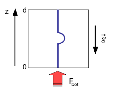
Our system is composed by a 2-D plane parallel layer of width . denotes a cartesian coordinate, pointing upward on the contrary of the constant gravity field . The gas is assumed to be monatomic and perfect, so its equation of state is given by
| (1) |
where , and respectively denote pressure, density and temperature, is the ideal gas constant and the ratio of specific heats and .
We are interested in small perturbations around an equilibrium state, that is, any physical quantity is expanded around its mean value as
| (2) |
where is an Eulerian perturbation. Linearized continuity, momentum and energy equations for the perturbations in a non-adiabatic case are given by (e.g. Unno et al. 1989)
| (3) |
where and denote the velocity, density, temperature and radiative flux perturbations, respectively. The kinematic viscosity is supposed to be constant and denotes the traceless rate-of-strain tensor given by
| (4) |
We seek normal modes with a time-dependence of the form , where . The real part denotes the growing () or damping () rate whereas the imaginary part denotes the frequency. We now assume that the layer is fully radiative which, under the diffusion approximation, leads to the following expression of the radiative flux perturbation
| (5) |
where denotes the radiative conductivity and its Eulerian perturbation. This perturbation can be related in a general way to the temperature one by
| (6) |
Finally, we impose the following boundary conditions
| (7) |
which correspond to rigid walls at both limits of the domain, a perfect conductor at the bottom and a perfect insulator at the top.
3 Conditions for instability
3.1 A first condition derived from the work integral
We recall that the main aim of this work is to clarify the favourable conditions which may sustain unstable radial modes in a plane parallel layer. An advisable mean to study the physics of such instability is the work integral. In the following, we are going to assume that transformations are quasi-adiabatic. This approximation is sufficient in the deeper layers of a star but becomes no longer valid near its surface where non-adiabatic effects dominate. Nevertheless, this approximation is useful when one wants to have an idea of the stability properties of an oscillation mode.
Using the work integral formalism in the quasi-adiabatic limit, we demonstrate in Appendix A.1 the following expression for the damping or growing rate of an eigenmode
| (8) |
where the symbol means the real part. We thus see that the sign of only depends on the numerator which, under the diffusion approximation, Eq. (5), leads to
| (9) |
The main driving term in this expression is because it represents the dynamical variation of opacity during an oscillation cycle, which is the cause of -mechanism. We thus neglect to get
| (10) |
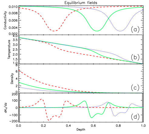
As we can see in Fig. 3b, the equilibrium temperature is an almost linear function of , except in the vicinity of the conductivity hollow. Therefore, is almost constant thus we have
| (11) |
With Eq. (6), we have . As we are interested in low order modes we assume that is dominated by . The same approximation will be done in Eq. (17). We then obtain
| (12) |
Let us now consider a compression phase corresponding to and . As , a necessary condition to obtain unstable modes with is then
| (13) |
In variable stars, this condition can occur in ionisation regions. Indeed, opacity tables clearly show that these regions are associated with large “bumps” in opacity (e.g. the review of Carson 1976; Seaton & Badnell 2004). With Eq. (13), one can obtain unstable modes if driving prevails over damping. This result has the following physical meaning: if the radiative conductivity decreases during a compression phase, then some part of the radiative flux is blocked and some energy is stored during compression contributing to increase the ratio of ionised matter. During the decompression phase, this extra energy is released under mechanical work to the environment and can excite the oscillations. It works as Eddington predicted when he imagined a thermal heat engine to justify Cepheids’ oscillations (Eddington 1917).
3.2 A second condition derived from the so-called “transition region”
In the previous paragraph, we have recalled a necessary condition to obtain unstable modes (Eq. 13). Nevertheless, the demonstration was made under the quasi-adiabatic approximation which fails near the surface. As a consequence, we cannot know if the driving caused by ionisation regions can prevail over other damping regions. Indeed, ionisation regions where Eq. (13) is satisfied are very thin compared to the whole atmosphere of a star and thus the influence of the damping regions on the instability remains questioning at this stage. Hereafter, we will essentially follow Cox’s demonstration (e.g. Cox 1980; Christensen-Dalsgaard 2003).
In Lagrangian variables, the energy equation can be written as
| (14) |
where the symbol means Lagrangian perturbations. As we consider a 1-D box, we simply have
| (15) |
Let us integrate between a given height and the surface to get
| (16) |
where is the variation of between the considered point and the surface, is an average of over this region and is a characteristic dynamical timescale (the pulsation period of the fundamental mode, typically). As we are principally interested in the study of low order modes (i.e. the fundamental one), we assume that the eigenvectors are almost constant (e.g. Cox 1980). As a consequence, one obtains
| (17) |
where expresses an average of the eigenfunctions. Noting that
| (18) |
leads to
| (19) |
where
| (20) |
has the following physical meaning: it represents the ratio of the thermal energy embedded between the considered point and the surface to the energy radiated during an oscillation period222 can also be interpreted as the ratio of the local thermal timescale to the dynamical one.. A second instability criterion can then be derived from the value of this quantity :
-
•
If the considered point is too deep in the star, the local thermal timescale is longer than the dynamical one and . As a consequence, pulsation has no influence on the energy release and the adiabatic approximation333One can notice that the “adiabatic” approximation means here that deeply in the layer the mode has an adiabatic behaviour whereas next to the surface it remains strongly non-adiabatic. is well-suited in this case.
-
•
On the contrary, if the considered point is next to the surface, then is very small and . As a consequence, the energy content (and the corresponding mass content) is too weak to influence the radiative flux and the luminosity perturbation is said to be frozen in. It means that the radiative flux perturbation doesn’t vary anymore in this region.
-
•
Between these two regions, can be which defines a zone called the transition region separating the adiabatic interior from the strongly non-adiabatic surface, that is,
(21)
King & Cox (1968) have first determined the temperature associated with this transition region for different Cepheids’ models. For the fundamental mode, they have obtained K while the transition lies nearer the surface for higher order modes.
The corresponding positions of ionisation regions and transition ones are therefore crucial for the instability (Gilliland et al. 1998). Indeed, if they overlap -it corresponds to the instability strip- the bottom of the ionisation region strongly contributes to driving because it acts in a quasi-adiabatic place. On the contrary, its top is in a strongly non-adiabatic region where the luminosity is frozen in. As a consequence, the zone over ionisation region is not damping and driving prevails in this case: modes become unstable (see e.g. Cox (1980) for a more detailed description).
4 Our hydrodynamical model
4.1 The choice of the radiative conductivity profile
Strictly speaking, radiative conductivity depends both on temperature and density as diffusion approximation gives (e.g. Mihalas & Weibel Mihalas 1984)
| (23) |
where denotes Stefan-Boltzmann’s constant. Kramer’s laws constitute good approximations of opacity laws with
| (24) |
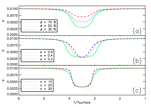
where, for example, and for the free-free opacity (e.g. Hansen & Kawaler 1994). As shown in the Introduction and in §2, we simply consider here a constant radiative conductivity on which a hollow representing a bump in opacity is added. This simple approach is an easy way to reproduce the physical conditions propitious to -mechanism while keeping the ability to quickly change the hollow amplitude, slope or width and achieving so an efficient parametric study of the instability. As a consequence, the radiative conductivity is given by444This -profile may appear quite intricate, compared e.g. to a gaussian-like one, but it allows us to change almost independently the hollow parameters (i.e. changing its amplitude while keeping its width).
| (25) |
with
| (26) |
and
-
•
is the position of the hollow in temperature.
-
•
and are the conductivity extrema, being the corresponding relative amplitude.
-
•
represents the slope of the hollow.
-
•
represents the half of the full width at half maximum (i.e. ) of the hollow.
Examples of common values of these parameters are given in Fig. 2.
.
4.2 The equilibrium setup
Hydrostatic and radiative equilibria in the diffusion limit are given by
| (27) |
Assuming a constant radiative flux at the bottom of the layer leads to
| (28) |
Let us choose the depth of the layer as the length scale and the temperature at the top of the layer as the temperature scale, i.e and . Moreover, the top density is chosen as the density scale (), velocity is given in units of , gravity in units of , pressure in units of , while radiative conductivity is given in units of . Corresponding radiative flux unit is then . The dimensionless equations then become
| (29) |
The set of equations (29) can be written in matrix form as
| (30) |
where is the equilibrium field vector and are differential operators. One notes that the RHS, , depends on the eigenvector itself through the terms and , which means solving a nonlinear problem.
Finally, tildes on equilibrium fields emphasise dimensionless quantities but they will be dropped for clarity in the following.
4.3 About Schwartzschild’s criterion in our model
It is important to keep our box entirely radiative. That is why, we must take care of Schwartzschild’s criterion (e.g. Chandrasekhar 1961)
| (31) |
If this inequality is ensured, then the layer is fully radiative. In our dimensionless units, this condition becomes
| (32) |
meaning that large variations in temperature through the domain necessarily require large values for the dimensionless gravity field .
4.4 Back to the radial oscillations equations
To simplify the general system of oscillations equations (3) we first define the following new variables
| (33) |
Then, by using Eq. (29) and substituting the conductivity equation into the energy one (see Appendix B), one gets
| (34) |
We then adopt the same dimensionless quantities used in the equilibrium equations (29)
| (35) |
where denotes the vertical velocity, the radiative diffusivity and the viscous dissipative term is given by
| (36) |
This system (35) may formally be written as a generalised eigenvalue problem
| (37) |
where is the complex eigenvalue associated with the eigenvector while denote differential operators.
Finally the set of boundary conditions (7) written for is
| (38) |
4.5 The numerical methods
We solve the two linear algebra problems (30) and (37-38) using the LSB code (Linear Solver Builder, Valdettaro et al. 2007). Both problems are discretized on the Gauss-Lobatto grid associated with Chebyshev’s polynomials leading to two distinct numerical problems:
-
1.
the equilibrium model: the computation of the equilibrium structure requires to solve a nonlinear problem. One way to do that is to use the so-called “Picard’s method” based on the fixed-point algorithm (Hairer et al. 1993; Fukushima 1997). It consists in solving our set of first-order ordinary differential equations by successive iterations, that is, we advance
(39) This scheme converges quite well provided that the initial guess is not “too far” from the solution and that nonlinearities are weak.
- 2.
5 Results
In Eq. (32), we have shown that the temperature contrast across the layer (and also the associated density and pressure ones) is limited by the gravity field . It may however be judicious not to restrict ourselves to small density contrasts as the mass involved between the conductivity hollow and the surface, that is , enters in one of the two favourable criteria for the instability, see Eq. (21). We will therefore consider in the following a “convenient” value .
Moreover, we have to keep as small as possible the radiative conductivity as we want to avoid too large values of diffusivity , that is, we do not want to deviate too much from conditions of the applying of quasi-adiabatic developments. We therefore choose . As a consequence, the system (29) combined with Schwartzschild’s criterion (32) restrict the possible values of the imposed bottom flux and we thus set in the following. Using mild spatial resolutions, we choose a conservative value for the kinematic viscosity, that is, .
5.1 Computation of equilibrium fields
To compute the equilibrium fields from second-order system (29), we must choose two different boundary conditions, one on temperature and one on pressure. Without loss of generality, we first set at the top of the layer. Second, as we are interested in having the transition region of the fundamental mode located in the layer middle, Eq. (21) has to be satisfied at that place. We have already said that and . Temperature value is fixed by , and its boundary condition. The pulsation period of the fundamental mode is roughly expressed by
| (40) |
where , denoting the mean sound speed, is related to the temperature contrast across the layer. Thus, the only parameter that we can change in Eq. (21) is . This value is directly linked to the boundary condition on density. In order to have a suitable -value in the box middle, we therefore decide to take at the top of the layer (corresponding to ).
Once chosen the values of the hollow parameters - and - we then solve the problem (29) on the Gauss-Lobatto grid to obtain the three equilibrium fields and . With these fields, it is possible to compute any physical quantities needed in the oscillations equations (35), e.g. or the diffusivity . Some examples of obtained equilibrium fields are given in Fig. 3 for three different positions of the conductivity hollow.
5.2 Computation of eigenmodes
With the different equilibrium quantities, we solve the eigenvalue problem (35) to get the whole spectrum of eigenvalues . Among them, it is possible to obtain the nearest eigenvalue from a guessed one using the iterative Arnoldi-Chebyshev algorithm. As an example, Fig. 4 brings out the eigenfunctions associated with the unstable fundamental mode.
In order to check the convergence of this mode, we also compute the spectra corresponding to the different eigenfunctions, see Fig. 5.

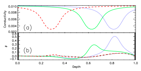
Finally, in order to determine the influence of the conductivity hollow on that fundamental eigenvector, we compute three eigenmodes with the different values of previously used in Fig. 3. The result is displayed in Fig. 6 for the temperature perturbation , where the case of a constant radiative conductivity profile (i.e. without a conductivity hollow) is superimposed:
-
•
The first case, corresponding to the dotted (blue) line, denotes a hot star where the ionisation region is close to the surface. The conductivity hollow has an influence on the temperature eigenfunction which is strongly deformed at its location. We will show in §5.4 that this deformation is not sufficient to destabilise this mode as the -criterion should also be taken into account (Eq. 21).
-
•
The second one, corresponding to the solid (green) line, emphasises a case where ionisation occurs approximately in the middle of the layer. The eigenvector is still deformed by the conductivity hollow.
-
•
The last case, corresponding to the dashed (red) line, denotes a cold star where ionisation region is far from the surface. For this hollow location, the dynamical timescale is very small compared to the local thermal one. As a consequence, thermodynamic transformations are quasi-adiabatic and non-adiabatic effects are negligible there. This is confirmed in Fig. 6b where the eigenmode is practically not deformed by the conductivity hollow. To enlighten this result, we have superimposed the case corresponding to a constant radiative conductivity (). The obtained temperature perturbations (the dot-dashed (black) line) are really next to the dashed (red) one, meaning that the hollow has a marginal effect on the mode stability.
We then show that the conductivity hollow has only an influence on the shape of the eigenmode in upper parts of our layer. In deeper regions, adiabatic thermodynamic transformations are overwhelming and the eigenvector is pretty unchanged by the variations in the conductivity profile.
5.3 Parametric surveys of the instability
As claimed in §4.1, our conductivity profile is well-suited to deal with a parametric study of the -mechanism, as its parameters and can easily be changed. We thus next introduce the three parametric surveys which allowed us to find the instability strips associated with the -mechanism.
5.3.1 The survey
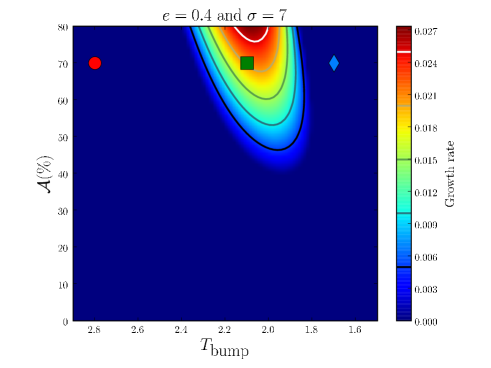
At first, we want to determine the influence of the hollow amplitude on stability. As a consequence, we choose a value for and and make and vary. For each value of these two parameters, we compute first the equilibrium fields and then, the eigenvalues with their corresponding eigenvectors. Unstable modes are extracted among all eigenvalues as their growth rate are positive. Fig. 7 displays the obtained instability strip:
-
•
Dark (blue) areas correspond to stable fundamental modes (i.e. with ).
-
•
Coloured areas correspond to unstable fundamental modes with the lighter the colour the bigger the growth rate.
Two major results can then be derived from this figure: (i) a particular region in our layer () seems to be propitious to the appearance of unstable modes, that is, one recovers the concept of transition region discussed in §3.2; (ii) a minimal amplitude in the hollow is required to get an instability ().
5.3.2 The survey
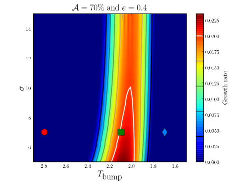
Next, we study the influence of the slope of the conductivity hollow on stability. We thus choose a value for the amplitude and width while making and vary. As for the previous survey, we plot in Fig. 8 the isocontours in growth rates but now in the plane .
We then found the same kind of areas than in Fig. 7, that is, an instability strip where modes are unstable (e.g. the coloured region) embedded in large (dark) regions where modes are stable. Nevertheless, the influence of the slope on stability is less significant than the amplitude one. In fact, the instability strip covers the same temperature range than in Fig.7, , but it becomes almost vertical as there is no critical value of to trigger off the destabilisation of the layer. In other words, there is a degeneracy in as this parameter is not affecting on the stability.
5.3.3 The survey
Finally, we study the influence of the hollow width on the stability by performing a survey in the -plane, while keeping constant and . Results are displayed in Fig. 9.
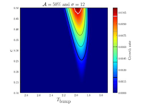
An instability strip of the same kind than the one shown in Fig. 7 is clearly visible as it exists a minimal value for the width from which the fundamental mode becomes unstable (). It means that narrow hollows are not sufficient to initiate the instability.
5.3.4 Summary of the surveys
These three parametric studies allow us to show the respective influence of the hollow parameters on the layer stability:
- •
-
•
Only the amplitude and width of the hollow have an influence on the stability as we found critical values for both of them, i.e. and . This can be linked to the condition (13) which entails that a precise shape in the conductivity profile is needed to get unstable modes. Moreover, the hollow slope is not a key control parameter as it does not modify the shape of the instability strip while varying.
We are now going to clarify these propitious conditions thanks to the work integral formalism.
5.4 Work integral in the non-adiabatic case
By generalising to the non-adiabatic case the demonstration done in Appendix A.1, we obtain the following expression for the exact (complex) eigenvalue
| (41) |
As the denominator is always positive, the sign of the real part only depends on the numerator one. To separate the regions of damping from the ones of driving, we thus plot the real part of the work integral in Fig. 10b.
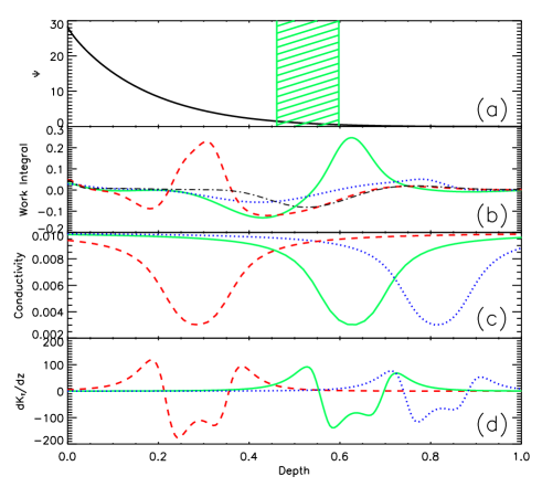
The work integral is really useful as it is possible to precisely check where the driving occurs. The criteria given in Eq. (22) predict that for a “sufficient” hollow, i.e. with a sufficient amplitude and width located in the transition region, the fundamental mode will be unstable. This result has already been checked thanks to the parametric study (Fig. 7 for example). With the work integral, we consider the same three particular modes studied before in Figs. 3 and 7:
-
•
The first one, plotted in dotted blue, expresses a case of a hot star where ionisation region is next to the surface. In this case, ionisation region is located in a place where density is really small, and thus . In Fig. 10b, we compare this case to the one with a constant radiative conductivity, for which and , and we can conclude that the conductivity hollow has a little influence on the work integral in this case: driving is unable to prevail over damping and .
-
•
In the second case, plotted in solid green, the radiative conductivity begins to decrease significantly at the location of the transition region where . As a consequence, driving is important in this place (Eq. 22). In addition, the radiative conductivity increase occurs in a place where non-adiabatic effects are already significant, i.e . This means that no damping will occur between the hollow position and the surface because the radiative flux perturbations are “frozen in”. Driving is overcoming damping in this case and thus, .
-
•
The third case, plotted in dashed red, denotes a cold star where ionisation region is located deeper in the stellar atmosphere where . As shown in Fig. 6, ionisation occurs there in a quasi-adiabatic place. As a consequence, excitation provided by the conductivity hollow cannot balance the damping arising in the layer, thus .
In conclusion, Fig. 10 illustrates both conditions given in Eq. (22): (i) it is first necessary to have to drive the oscillations. But this condition is not sufficient to sustain the -mechanism; (ii) indeed, the thermal engine underlying the conductivity hollow has to be located neither too deep in the star, nor too close to the surface. Therefore, only a specific range of effective temperatures allows the overlap of the transition and ionisation regions, which leads to the instability strips found in Figs. 7-9.
6 Direct Numerical Simulations
In order to confirm all of the instability strips arising in the previous linear stability analysis, we performed direct numerical simulations of the nonlinear problem. That is, starting from the most favourable setups found during the parametric surveys, we advanced in time the nonlinear hydrodynamic equations to check:
-
•
the onset of the instability sustained by the -mechanism and thus confirm the growth rates of the linear stability analysis.
-
•
the nonlinear saturation of the instability, which is of course not caught in the linear analysis, and have an estimation of the final amplitudes of modes.
All DNS have been done using the Pencil Code555See http://www.nordita.org/software/pencil-code/ and Brandenburg & Dobler (2002).. This non-conservative code is a high-order centered finite difference code (of the sixth order in space and third order in time) and conserved quantities are kept up to the discretization error of the scheme. On multiprocessor computers, it uses the MPI libraries (Message Passing Interface) which allow communications between processors and thus runs in parallel. Moreover, this code is a fully explicit one as the computation of the solution at time depends on the solution obtained at time before. The timestep is therefore limited by an usual Courant-Friedrichs-Levy (CFL) condition based on the consideration of the smallest physical timestep existing in the simulation as
| (42) |
where , and are constant coefficients depending on the spatial order of the scheme (see §19.2 in Press et al. 1992, hereafter PTVF92).
6.1 The needed of an implicit solver
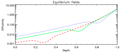
This CFL condition is clearly a problem in our case as the most favourable setups imply very large radiative diffusivities at the surface. Fig. 11 emphasises this point where the diffusivity profile is plotted for the three common hollows used in this work (). Because the -criterion (21) imposes a weak value of and hence of the top density, one gets large surface values for the radiative diffusivity in all cases. It means that the corresponding radiative diffusion timestep entering in Eq. (42) will be the smallest one and will impose a very small timestep . As an example, if we consider a typical spatial resolution of (i.e. 256 gridpoints in each direction), we obtain whereas the dynamics of the layer is rather constrained by the sound speed of which the dynamical timescale is .
It is therefore numerically prohibitive to reach the nonlinear saturation of excited acoustic modes with such an explicit solver. To limit the number of iteration, we have decided to solve the diffusion of temperature implicitly. In fact, as implicit schemes are unconditionally stable, we have no more constraints on the timestep coming from radiative diffusion and thus the CFL becomes
| (43) |
giving for the same resolution .
6.2 The Alternate Direction Implicit (ADI) scheme
In order to solve the temperature equation, we adopt the time-split formulation given in Malagoli et al. (1995). We thus solve first explicitly the three hydrodynamic equations, i.e. density, velocity and temperature, but without solving the radiative diffusion term at this step. We then solve the temperature diffusion with the intermediate temperature treated as a source term.
The time advance of the diffusion temperature equation is treated implicitly in the form
| (44) |
where the radiative diffusion term is expressed by
| (45) |
could be directly dealt with a Cranck-Nicholson method and a single matrix inversion with, for instance, a Successive Over Relaxation (SOR) method. For a 2-D problem, this approach forces us to invert a very sparse matrix (e.g. §19.5 in PTVF92). That is why we have decided to implement an Alternate Direction Implicit (ADI) scheme which relies on operator splitting theory which is frequently used in diffusion problems (e.g. §19.3 in PTVF92; Dendy 1977; Masalkar 1994). It allows us to deal with tridiagonal matrices (or cyclic ones depending on the boundary conditions used) by solving implicitly both directions successively.
To treat implicitly the nonlinear terms (i.e. ) we have adopted the following approximation commonly called Rosenbrock’s method (Saarikoski et al. 1997; Witelski & Bowen 2003)
| (46) |
where denotes the Jacobian matrix associated with the operator . Expanding Eq. (44) in each direction thus leads to
| (47) |
where and are the identity matrix, a cyclic one and a tridiagonal one, respectively.
6.3 Results
All 2D-simulations were carried out using a mean resolution and a constant kinematic viscosity . In order to avoid as much as possible the propagation of nonradial modes (Mulet-Marquis et al. 2007), we chose a “small” box with an aspect ratio . Indeed, if we refer to classical hydrodynamic instabilities, the critical horizontal wavelength from which the instability develops is generally a bit larger than the vertical extent of the domain. As an example, in the Rayleigh-Bénard convection (Chandrasekhar 1961) or in the compressible polytrope (Gough et al. 1976).
6.3.1 Growth rates from the DNS
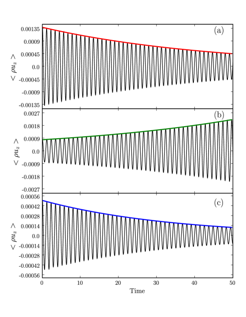
Fig. 12 emphasises the temporal evolution of the mean momentum (where is an average over the entire box) for the three common equilibrium setups (the red, green and blue ones corresponding to ). Only one case appears to be unstable as:
| Rel. err. | |||
|---|---|---|---|
| red | |||
| green | |||
| blue |
-
•
The first (red) setup expresses the case of a cold star where ionisation region is deep. The linear stability analysis achieved before predicts that no excitation will occur in this case (the red circle in Fig. 7 is well outside the instability strip). As seen in Fig. 12a, this result is confirmed by the nonlinear simulation as the mean vertical momentum decreases with time. Moreover, the damping rate calculated with LSB (superimposed as a red line) is reproduced with a great agreement in this simulation (Table 1).
-
•
The second (green) setup denotes the case where the -mechanism is efficient. As a consequence, the fundamental p-mode is expected to be unstable (the green square inside the instability strip in Fig. 7). The DNS confirms this excitation (Fig. 12b) and the growth rate is the same as the predicted one (Table 1).
-
•
The third (blue) one corresponds to a hot star where ionisation is next to the surface. In this case, damping phenomena prevail over excitation and the fundamental mode is stable (the blue diamond outside the instability strip in Fig. 7). One more time, the result is confirmed by the DNS (see Fig .12c and Table 1).
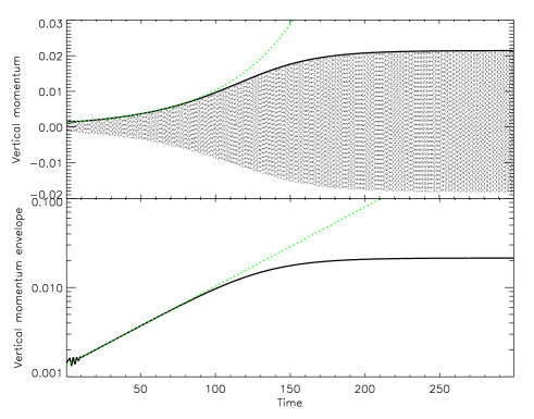
In Fig. 13, we have integrated the DNS from the initial green setup with till the approach to the nonlinear limit cycle stability, that is, the nonlinear saturation. The (green) dotted line corresponds to the theoretical growth rate given in Table 1, that is, . The saturation of this mode appears to be achieved around time , which roughly corresponds to mode periods. Such time interval is compatible with the characteristic timescale of the instability given by . Finally, the amplitude reached at the end of the saturation is about . A careful study of the modes saturation is beyond the scope of this paper and will be developed in future works.
6.3.2 Vertical profiles
The good agreement between the theoretical and DNS growth rates shown in Table 1 marks a first success in reproducing the -mechanism in our simulations. We next address the point of the modes structure by computing the vertical profiles from the DNS and comparing them to the eigenvectors of the linear stability analysis.
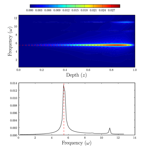
In Fig. 14, we have performed an horizontal and temporal Fourier transforms of the vertical velocity field and plotted the resulting power spectrum at in the plane -plane. With this method, we are able to determine exactly which acoustic modes are excited or not in our numerical experiment as they emerge in this plane as “shark fin” peaks around given frequencies (see Dintrans & Brandenburg 2004). That is indeed what is displayed in Fig. 14 where the radial acoustic mode with a frequency is excited and the agreement with the linear eigenfrequency is remarkable. The second overtone with also appears in the -plane, with still a good agreement between the linear stability analysis and the DNS. In fact, one can note that this frequency is almost twice the fundamental mode one. It means that a resonance-like interaction occurs between these two modes: the -mechanism excites the fundamental mode and a nonlinear interaction transfers some energy between this mode and the second damped overtone, leading to the nonlinear saturation.
As we have computed, thanks to LSB, the eigenfunctions from a given equilibrium setup (see Fig. 4), one can compare them to the vertical velocity deduced from the power spectra in Fig. 14. That is what is displayed in Fig. 15 where a mean profile around the frequency has been computed. The DNS profile and the linear stability analysis one perfectly overlap meaning that we both have an agreement on the temporal (i.e. the frequency) and spatial (i.e. the pattern) scales of this mode.

7 Conclusion
We have modeled -mechanism in Cepheids by a similar physical problem: the propagation of radial acoustic waves in a partially ionised shell. Our model consists in a perfect gas embedded in an entirely radiative layer and the ionisation region has been depicted by a configurable hollow in radiative conductivity. This approach allows to quickly change the shape and location of this ionised region in the layer through the hollow parameters and (Eqs. 25-26). We first have checked that a hollow with a sufficient amplitude and width may lead to
| (48) |
which corresponds to the classical instability criterion derived from the work integral and quasi-adiabatic considerations. Nevertheless, another condition is needed to obtain a thermal heat engine in Eddington’s sense: the ionisation region has to be located at a certain place in the layer, neither to deep nor to close to the surface. We have shown that this propitious area is located in the so-called transition zone separating the quasi-adiabatic interior from the strongly non-adiabatic surface. This thermodynamical criterion can be summarised by
| (49) |
With this second criterion, appropriate boundary conditions have been chosen in order to have a transition region in the middle of our box for the fundamental acoustic mode. Both radiative and hydrostatic equilibria have then been discretized on the (spectral) Gauss-Lobatto grid and solutions have been computed thanks to a linear solver. Once done, we have performed a linear stability analysis by computing the whole spectrum as well as associated eigenvectors for the radial oscillations equations.
The main advantage of our approach lies in its ability to make the parameters of the conductivity hollow vary. The major result of parametric surveys is the checking of the previous conditions by way of the appearing of instability strips: only configurations satisfying both conditions (48-49) have led to unstable fundamental modes (e.g. Figs. 7 and 10).
Then, these most favourable setups found in the linear stability analysis have been the starting points of our first 2-D (nonlinear) DNS of -mechanism. However, because of a too restrictive Courant-Friedrichs-Levy (CFL) condition at the surface, these setups were not well-suited for a fully explicit code such as the Pencil Code one. We therefore have developed a new implicit module to deal with the radiative diffusion term and thus soften the CFL constraint. These DNS have confirmed with a great agreement both growth rates and structures of linearly unstable modes (see Figs. 13 and 15). Moreover, we have been able to reach the nonlinear saturation which involves an intricate coupling between the fundamental mode and (at least) the damped second overtone of which the period is a multiple of the fundamental one.
This work constitutes a first step in our Cepheids’ project devoted to the modelling of the convection-pulsation interaction in the coldest Cepheids close to the red edge of the instability strip. Indeed, it is well known that convection occurs in a non-negligible part of these stars and modify the pulsation properties. For now, models based on time-dependent convection theories reproduce quite well the position of this red edge or, say, observational periods and light curves (YKB98; Bono et al. 1999). However, they involve many free parameters which are either fitted to the observations or hardly constrained by theoretical values, leading to almost similar results for different parameter sets (Kolláth et al. 2002; Szabó et al. 2007).
Despite their own limitations (their weak contrasts in pressure through the computational domain or their thermal timescale problem, see e.g. Brandenburg et al. (2000)), DNS are without a doubt a good way to address this convection-pulsation interaction as they fully take into account the crucial nonlinearities. With a conductivity profile solely based on temperature (Eq. 25), it is easy to locally shape one (or several) convective zone by increasing the temperature gradient above the adiabatic one. Indeed, as an ionisation region corresponds to a local increase in opacity, it is well known that convection can develop there. This occurs in cold Cepheids where two separate convectively unstable regions superimpose with the HeI/H and HeII ionisation regions. By adjusting in DNS the convective zone width or the strength of gravity, it will be possible to match the (local) turnover timescale of convection with the mean mode period, and then to study the coupling between convection and pulsation.
Acknowledgements.
Calculations were carried out on the CalMip machine of the “Centre Interuniversitaire de Calcul de Toulouse” (CICT) which is gratefully acknowledged. It is also a pleasure to thank Isabelle Baraffe, Fabien Dubuffet, Marie-Jo Goupil and Michel Rieutord for their fruitful comments.Appendix A Work Integral
A.1 Using the quasi-adiabatic approximation
In the energy equation in Syst. (3), we can first separate adiabatic terms from non-adiabatic ones as
| (50) |
and, by using the ideal gas equation of state (1),
| (51) |
This equation corresponds to the pressure perturbation due to both adiabatic and non-adiabatic oscillations. The momentum equation in Syst. (3) then becomes
| (52) |
This equation can formally be written as a generalised eigenvalue problem with a perturbation operator
| (53) |
where and are caused by the perturbation operator (here the non-adiabatic effects). can then be obtained from a first-order perturbation analysis equivalent to these done in quantum mechanics (e.g. Bender & Orszag 1978; Dyson & Schutz 1979)
| (54) |
where the symbol means the following dot product (e.g. Lynden-Bell & Ostriker 1967)
| (55) |
We thus obtain the expression for the eigenvalue perturbation
| (56) |
We can go a step further using
| (57) |
of which the first term in the RHS vanishes due to the rigid boundaries for the velocity as
| (58) |
The second term in the RHS can also be simplified by using the continuity equation
| (59) |
where is the Lagrangian perturbation of density. We finally get the expression for the eigenvalue perturbation in the non-adiabatic case as
| (60) |
where we have assumed that the adiabatic eigenmode is purely imaginary, that is , and thus . We note that corresponds to the damping (or growing) rate of a non-adiabatic mode, commonly written .
A.2 A thermodynamical approach
It is also possible to derive Eq. (60) by energetic considerations. Hereafter, we will essentially follow Hansen’s demonstration (Hansen & Kawaler 1994). Let us adopt a thin shell of mass at a certain radius. During a complete cycle of oscillations the work done by the shell on its surroundings is linked to the internal energy and heat gained by this shell through the first principle of thermodynamics
| (61) |
Integrating over a cycle of oscillations leads to
| (62) |
We are now going to suppose that the oscillation mechanism is quasi-adiabatic. It implies that every thin shell behaves as a Carnot-like heat engine where each process is reversible and the shell comes back to its initial position after each cycle of oscillations. Internal energy being a state variable, one gets hence
| (63) |
Now one applies the second principle of thermodynamics claiming that
| (64) |
After some time elapsed, we have and then
| (65) |
as a first-order approximation, with for the same reason than . We thus write
| (67) |
which leads to the total work integrated over mass shells
| (68) |
If , the star produces work over a cycle of oscillations and the initial perturbation will grow. In this case, the star is driving pulsation which is thus unstable. It may occur when shells gain heat (i.e. ) during compression phases (i.e. ) and this is the so-called “valve-mechanism” proposed by Eddington (1917).
Let us write the energy equation in the form
| (69) |
and substitute it in Eq. (68)
| (70) |
Kinetic energy over a period of oscillations is given by
Appendix B The radiative term in energy equation
Radiative flux perturbations can be written as
| (73) |
By assuming and using Eq. (6), it entails
| (74) |
We then expand with equilibrium equations (29) as
| (75) |
and thus obtain
| (76) |
Finally, one gets
| (77) |
References
- Arnoldi (1951) Arnoldi, W. E. 1951, QApMa, 9, 17
- Baker & Kippenhahn (1962) Baker, N. & Kippenhahn, R. 1962, Zeitschrift für Astrophysik, 54, 114
- Baker & Kippenhahn (1965) Baker, N. & Kippenhahn, R. 1965, ApJ, 142, 868
- Bender & Orszag (1978) Bender, C. M. & Orszag, S. A. 1978, Advanced Mathematical Methods for Scientists and Engineers (Advanced Mathematical Methods for Scientists and Engineers, New York: McGraw-Hill, 1978)
- Böhm-Vitense (1958) Böhm-Vitense, E. 1958, Zeitschrift für Astrophysik, 46, 108
- Bono et al. (1999) Bono, G., Marconi, M., & Stellingwerf, R. F. 1999, ApJS, 122, 167
- Brandenburg & Dobler (2002) Brandenburg, A. & Dobler, W. 2002, CoPhC, 147, 471, [arXiv:physics/0111569]
- Brandenburg et al. (2000) Brandenburg, A., Nordlund, A., & Stein, R. F. 2000, Geophysical & Astrophysical Convection, ed. P. A. Fox & R. M. Kerr (New York: Gordon and Breach Science Publishers)
- Buchler (1997) Buchler, J. R. 1997, in Variables Stars and the Astrophysical Returns of the Microlensing Surveys, ed. R. Ferlet, J.-P. Maillard, & B. Raban, 181
- Carson (1976) Carson, T. R. 1976, ARA&A, 14, 95
- Chandrasekhar (1961) Chandrasekhar, S. 1961, Hydrodynamic and hydromagnetic stability (International Series of Monographs on Physics, Oxford: Clarendon, 1961)
- Christensen-Dalsgaard (2003) Christensen-Dalsgaard, J. 2003, Lecture Notes on Stellar Oscillations (Physical and Astronomical Institute of Aarhus University)
- Cox (1958) Cox, J. P. 1958, ApJ, 127, 194
- Cox (1963) Cox, J. P. 1963, ApJ, 138, 487
- Cox (1980) Cox, J. P. 1980, Theory of stellar pulsation (Research supported by the National Science Foundation Princeton, NJ, Princeton University Press, 1980. 393 p.)
- Dendy (1977) Dendy, J. E. 1977, SJNA., 14, 313
- Dintrans & Brandenburg (2004) Dintrans, B. & Brandenburg, A. 2004, A&A, 421, 775, [arXiv:astro-ph/0311094]
- Dyson & Schutz (1979) Dyson, J. & Schutz, B. F. 1979, Royal Society of London Proceedings Series A, 368, 389
- Eddington (1917) Eddington, A. S. 1917, The Observatory, 40, 290
- Fukushima (1997) Fukushima, T. 1997, AJ, 113, 1909
- Gautschy & Saio (1996) Gautschy, A. & Saio, H. 1996, ARA&A, 34, 551
- Gehmeyr & Winkler (1992) Gehmeyr, M. & Winkler, K.-H. A. 1992, A&A, 253, 101
- Gilliland et al. (1998) Gilliland, R. L., Bono, G., Edmonds, P. D., et al. 1998, ApJ, 507, 818
- Gough (1977) Gough, D. O. 1977, ApJ, 214, 196
- Gough et al. (1976) Gough, D. O., Moore, D. R., Spiegel, E. A., & Weiss, N. O. 1976, ApJ, 206, 536
- Hairer et al. (1993) Hairer, E., Norsett, S. P., & Wanner, G. 1993, Solving Ordinary Differential Equations I: Nonstiff Problems (Springer-Verlag: Berlin Heidelberg New York)
- Hansen & Kawaler (1994) Hansen, C. J. & Kawaler, S. D. 1994, Stellar Interiors. Physical Principles, Structure, and Evolution. (Stellar Interiors. Physical Principles, Structure, and Evolution, XIII, 445 pp. 84 figs. 3 1/2” diskette. Springer-Verlag Berlin Heidelberg New York. Also Astronomy and Astrophysics Library)
- King & Cox (1968) King, D. S. & Cox, J. P. 1968, PASP, 80, 365
- Kolláth et al. (2002) Kolláth, Z., Buchler, J. R., Szabó, R., & Csubry, Z. 2002, A&A, 385, 932, [arXiv:astro-ph/0110076]
- Kuhfuß (1986) Kuhfuß, R. 1986, A&A, 160, 116
- Lynden-Bell & Ostriker (1967) Lynden-Bell, D. & Ostriker, J. P. 1967, MNRAS, 136, 293
- Malagoli et al. (1995) Malagoli, A., Dubey, A., Cattaneo, F., & Levine, D. 1995, A Portable and Efficient Parallel Code for Astrophysical Fluid Dynamics, [http://astro.uchicago.edu/Computing/On_Line/cfd95/camelse.html]
- Masalkar (1994) Masalkar, P. J. 1994, Optik, 4, 168
- Mihalas & Weibel Mihalas (1984) Mihalas, D. & Weibel Mihalas, B. 1984, Foundations of radiation hydrodynamics (New York: Oxford University Press, 1984)
- Moler & Stewart (1973) Moler, C. B. & Stewart, G. W. 1973, SJNA., 10, 241
- Mulet-Marquis et al. (2007) Mulet-Marquis, C., Glatzel, W., Baraffe, I., & Winisdoerffer, C. 2007, A&A, 465, 937, [arXiv:astro-ph/0701371]
- Press et al. (1992) Press, W. H., Teukolsky, S. A., Vetterling, W. T., & Flannery, B. P. 1992, Numerical recipes in FORTRAN. The art of scientific computing (Cambridge: University Press, 1992, 2nd ed.), PTVF92
- Saad (1992) Saad, Y. 1992, Numerical Methods for Large Eigenvalue Problems (New York: Halsted Press)
- Saarikoski et al. (1997) Saarikoski, H., Salmio, R. P., Saarinen, J., Eirola, T., & Tervonen, A. 1997, OptCo, 134, 362
- Seaton & Badnell (2004) Seaton, M. J. & Badnell, N. R. 2004, MNRAS, 354, 457, [arXiv:astro-ph/0404437]
- Stellingwerf (1982) Stellingwerf, R. F. 1982, ApJ, 262, 330
- Szabó et al. (2007) Szabó, R., Buchler, J. R., & Bartee, J. 2007, ApJ, 667, 1150, [arXiv:astro-ph/0703568]
- Unno (1967) Unno, W. 1967, PASJ, 19, 140
- Unno et al. (1989) Unno, W., Osaki, Y., Ando, H., Saio, H., & Shibahashi, H. 1989, Nonradial oscillations of stars (Nonradial oscillations of stars, Tokyo: University of Tokyo Press, 1989, 2nd ed.)
- Valdettaro et al. (2007) Valdettaro, L., Rieutord, M., Braconnier, T., & Fraysse, V. 2007, JCoAM, 205, 382, [arXiv:physics/0604219]
- Vitense (1953) Vitense, E. 1953, Zeitschrift für Astrophysik, 32, 135
- Witelski & Bowen (2003) Witelski, T. P. & Bowen, M. 2003, ApNM., 45, 331
- Wuchterl & Feuchtinger (1998) Wuchterl, G. & Feuchtinger, M. U. 1998, A&A, 340, 419
- Yecko & Kollath (1998) Yecko, P. & Kollath, Z. 1998, in Astronomical Society of the Pacific Conference Series, Vol. 135, A Half Century of Stellar Pulsation Interpretation, ed. P. A. Bradley & J. A. Guzik, 94
- Yecko et al. (1998) Yecko, P. A., Kolláth, Z., & Buchler, J. R. 1998, A&A, 336, 553, [arXiv:astro-ph/9804124], YKB98
- Zhevakin (1953) Zhevakin, S. A. 1953, Russ. A. J., 30, 161
- Zhevakin (1963) Zhevakin, S. A. 1963, ARA&A, 1, 367