Förster mechanism of electron-driven proton pump

Anatoly Yu. Smirnov1,2, Lev G. Mourokh1,3,4, and Franco Nori1,5 1 Frontier Research System, The Institute of Physical and Chemical Research (RIKEN), Wako-shi, Saitama, 351-0198, Japan
2 CREST, Japan Science and Technology Agency, Kawaguchi, Saitama, 332-0012, Japan
3 Department of Physics, Queens College, The City University of New York, Flushing, New York 11367, USA
4 Department of Engineering Science and Physics, College of Staten Island, The City University of New York, Staten Island, New York 10314, USA
5 Center for Theoretical Physics, Physics Department, The University of Michigan, Ann Arbor, MI 48109-1040, USA
Abstract

We examine a simple model of proton pumping through the inner membrane of mitochondria in the living cell. We demonstrate that the pumping process can be described using approaches of condensed matter physics. In the framework of this model, we show that the resonant Förster-type energy exchange due to electron-proton Coulomb interaction can provide an unidirectional flow of protons against an electrochemical proton gradient, thereby accomplishing proton pumping. The dependence of this effect on temperature as well as electron and proton voltage build-ups are obtained taking into account electrostatic forces and noise in the environment. We find that the proton pump works with maximum efficiency in the range of temperatures and transmembrane electrochemical potentials which correspond to the parameters of living cells.

pacs:
87.16.Ac, 87.16 Uv, 73.63.-b

I Introduction

A living cell can be considered as a tiny electrical battery with a transmembrane potential difference of order $-70$ mV (with a negatively charged interior). Even a higher potential, $\Delta V\sim-200$ mV, is applied to the inner membrane of a mitochondrion, an organelle, which produces most of the energy consumed by the cell. Alberts02 ; Wik04 ; Brand06 . To create and maintain such an electrical potential, mitochondria employ numerous proton pumps converting energy of electrons into an electrochemical proton gradient that is harnessed thereafter to drive the synthesis of adenosine triphosphate (ATP) molecules. Translocation of protons across the inner membrane of mitochondria is performed by the enzyme cytochrome $c$ oxidase (COX). Although crystal structure of COX is known in detail, a molecular mechanism of the redox-driven proton pumping remains a mystery despite of the significant latest advances based on time-resolved optical and electrometric measurements Belev07 ; WV07 .

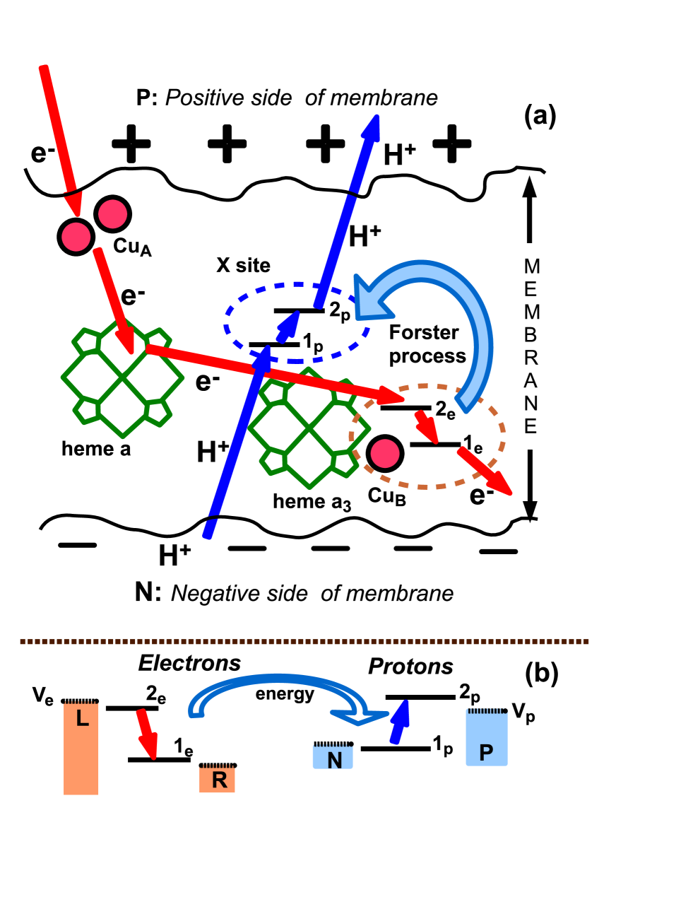
The electron transport chain of COX consists of four metal redox centers, ${\rm Cu}_{A}$, heme $a$, heme $a_{3}$, and ${\rm Cu}_{B}$ Brand06 ; Papa04 ; Bloch04 . The process starts when the mobile electron carrier, cytochrome $c$, moving from the positively charged P-side of the membrane, donates a high-energy electron to a dinuclear copper site, ${\rm Cu}_{A}$ (see Fig.1). After that, the electron proceeds to the heme $a$ with a subsequent transfer to the binuclear center formed by heme $a_{3}$ and a copper ion ${\rm Cu}_{B}$, where the dioxygen molecule ${\rm O}_{2}$ is reduced to water. To produce two molecules of water in the catalytic cycle with four electrons $(e^{-})$ Stuch06 ,

$${\rm O}_{2}+8~{}{\rm H}^{+}_{\rm N}+4~{}e^{-}\rightarrow 2~{}{\rm H}_{2}{\rm O}+4~{}{\rm H}^{+}_{\rm P},$$

the cytochrome oxidase consumes 4 substrate (chemical) protons which are translocated from the negative N-side of the inner mitochondrion membrane to the binuclear center. In the process, four more protons (${\rm H}^{+}_{\rm N}$) are taken from the N-side and pumped to the positive side (${\rm H}^{+}_{\rm P}$). Here, subscripts N and P for the protons denote the location of the proton ${\rm H}^{+}$ at the negative (N) or positive (P) side of the membrane, respectively. A residue $E278$ (for the $Paracoccus~{}denitrificans$ enzyme) or a conserved glutamic acid, $Glu242$ (for the bovine enzyme WV07 ; WV06 ), located at the end of the so-called D-pathway BelNat06 , can serve as starting points for both substrate and pumped protons on their way from the N-side to the binuclear center. In the next phase, a proton is transferred to an unknown yet protonable pump site $X$ which is located on the P-side of the heme groups and electrostatically coupled to heme $a$ and to the binuclear iron-copper center $a_{3}/{\rm Cu}_{\rm B}$ Belev07 ; WV07 . On the final stage, the proton moves from the site X to the positive side of the membrane after uphill pumping. In the context of a pure electrostatic model proposed in Refs. Belev07 ; WV07 , the protonation of the site X leads to the equalization of electron energy levels in hemes $a$ and $a_{3}$ that facilitates a transfer of an electron from heme $a$ to the binuclear center. This electron attracts a substrate proton which moves from the N-side of the membrane to the site X, expelling the first, pre-pumped proton to the P-side. Detailed density functional and electrostatics studies of this and other models have been performed in SiegJPC03 ; Stuch06 ; Blom06 ; Sieg07 ; Ols07 ; Hos06 . However, a mechanism of energy transmission from electrons to protons resulting in an unidirectional translocation of protons against the concentration gradient is still uncertain. For better understanding of this phenomenon, it is useful to combine a comprehensive analysis of the energetic and spatial structure of enzymes with simple and physically transparent models.

In the present paper, we approach the problem taking into account the similarity of the electron-driven proton transfer to the quantum transport of electrons through nanostructures Wingr . The interaction between electrons and protons is described by a Coulomb potential, but, in addition to the standard electrostatic terms, we analyze effects of the Förster-type Coulomb exchange Forst65 on the resonant energy transduction between electron and proton subsystems. Each of the subsystems is supposed to have two active sites: $1_{e},2_{e}$ for electrons, and $1_{p},2_{p}$ for protons. We consider here the possibility when both electron sites belong to the same potential well, localized in the binuclear center $a_{3}/{\rm Cu}_{\rm B}$, while both active proton states $2_{p}$ and $1_{p}$ can be ascribed to the pump center X (see Fig.1). This positioning of active sites corresponds in some sense to the electrostatic model of Ref. WV07 , based on time-resolved measurements of electron transfer in COX enzyme Belev07 .

During the Förster process, an electron moves from the state $2_{e}$, which has a higher energy, to the state $1_{e}$, with a lower energy; whereas a proton jumps from the lower-energy state $1_{p}$ to the higher-energy state $2_{p}$ (see Fig. 1). The same mechanism is responsible for the Fluorescence Resonant Energy Transfer (FRET) in biological systems ForstBio , as well as for the exciton transfer in condensed matter Klim04 .

The Förster term originates from the matrix element of the Coulomb electron-proton potential between the overlapping wave functions of the electron states $2_{e}$ and $1_{e}$, and the overlapping wave functions of proton states $1_{p}$ and $2_{p}$ Gov05 . Calculations show that this term is directly proportional to the product of the dipole moments of electron and proton two-level systems, also inversely proportional to the cube of the distance between the electron and proton sites, and requires to satisfy resonant conditions for the energies of the electron and proton subsystems. Accordingly, the Förster term is much weaker than standard electrostatic terms. However, as a consequence of its overlapping origin, this term opens a new channel for simultaneous tunneling of electrons and protons, in addition to the direct tunneling. We demonstrate that it is the Förster-type coupling that results in an effective electron-proton energy transfer, followed by the proton pumping from the negative to the positive side of the inner mitochondria membrane.

The rest of the paper is structured as follows. Formulation of Hamiltonians and energetic spectra of the problem is presented in Section II. Expressions for electron and proton currents are obtained in Section III. In Section IV, we derive equations of motion for the density matrix. In Section V, these equations are solved numerically and the obtained dependencies of the proton current on temperature, electron and proton voltage build-ups, and deviation from the resonant conditions are discussed. Section VI contains our conclusions.

II Model Formulation

Electrons and protons on sites $\sigma=1,2$ are characterized by the Fermi operators $a_{\sigma}^{+},a_{\sigma}$, and $b_{\sigma}^{+},b_{\sigma}$, respectively, with the corresponding populations, $n_{\sigma}=a_{\sigma}^{+}a_{\sigma}$ and $N_{\sigma}=b_{\sigma}^{+}b_{\sigma}$ (we interchangeably use the notation “site” = “state”). We assume that each electron site or proton site can be occupied by a single particle, so the maximal populations can be, at most, one electron on each one of the two separate electron sites, and, at most, one proton on each one of the two separate proton sites. To describe the continuous flow of carriers through the system, we assume that the electron site 2 is coupled to the left (L) reservoir, which serves as a source of electrons, and the electron site 1 is coupled to the right reservoir (R) playing the role of drain. At the same time, the proton site 1 can be populated when protons jump from the reservoir located on the negative (N) side of the membrane. On the positive side of the membrane, there is another proton reservoir which serves to depopulate of the proton site 2 (see Fig. 1b). In the framework of this model, here we neglect the couplings between the electron site 1 and the reservoir L, and between the site 2 and the reservoir R. We also neglect the tunneling between the proton site 1 and the positive side of the membrane (P), as well as the tunneling between the proton site 2 and the negative side of the membrane (N).

The electrons in the reservoir (lead) $\alpha$ ($\alpha=L,R$) or the protons in the reservoir (lead) $\beta$ ($\beta=N,P$) can be characterized by additional parameters $k$ and $q$, respectively, which have meanings of wave vectors in condensed matter physics. To describe the electronic and protonic sources and drains, we introduce the electron creation and annihilation operators in the $\alpha$-lead as $c_{k\alpha}^{+},c_{k\alpha}$, and their proton counterparts for the $\beta$-lead as $d_{q\beta}^{+},d_{q\beta}$. The number of electrons in the $\alpha$-lead is determined by the operator $\sum_{k}n_{k\alpha}$, with $n_{k\alpha}=c_{k\alpha}^{+}c_{k\alpha},$ whereas the proton population of the $\beta$-lead is given by the operator $\sum_{q}N_{q\beta}$, with $N_{q\beta}=d_{q\beta}^{+}d_{q\beta}$. It is well-known that in real biological structures, couplings between the active sites $1,2$ and the reservoirs can be mediated by many bridge states, similar to the ${\rm Cu}_{\rm A}$-site and heme $a$, which can be subjected to conformational changes. Conformation changes can also provide a selectivity in coupling between the active sites and the leads Wik04 .

II.1 Electron and proton Hamiltonians

The Hamiltonian of the electron-proton system incorporates a term related to eigenenergies $\epsilon_{\sigma}^{(0)},E_{\sigma}^{(0)}$ of electrons and protons, respectively, located on the sites $\sigma=1,2$, as well as a term describing electron and proton energies $\epsilon_{k\alpha},E_{k\beta}$ of the leads $\alpha=L,R;\beta=N,P:$

$$H_{{\rm init}}=\sum_{\sigma}(\epsilon_{\sigma}^{(0)}n_{\sigma}+E_{\sigma}^{(0)}N_{\sigma})+\sum_{k\alpha}\epsilon_{k\alpha}c_{k\alpha}^{+}c_{k\alpha}+\sum_{q\beta}E_{q\beta}d_{q\beta}^{+}d_{q\beta}.$$ (1)

The Hamiltonian $H_{\rm dir}$,

$$H_{\rm dir}=-\Delta_{a}a_{2}^{+}a_{1}-\Delta_{a}^{*}a_{1}^{+}a_{2}-\Delta_{b}b_{2}^{+}b_{1}-\Delta_{b}^{*}b_{1}^{+}b_{2},$$ (2)

is responsible for the direct tunneling of electrons and protons between the corresponding sites 1 and 2, with the rates $\Delta_{a}$ and $\Delta_{b}.$ Notice that the direct tunneling has a highly non-resonant character since the energy levels of the sites 1 and 2 are well separated: $\epsilon_{2}^{(0)}-\epsilon_{1}^{(0)}\gg\Delta_{a},~{}E_{2}^{(0)}-E_{1}^{0)}\gg\Delta_{b}.$ To take into consideration the coupling of the active sites 1 and 2 to the corresponding reservoirs of electrons and protons, we introduce the tunneling Hamiltonian

$$H_{\rm tun}=-\sum_{k}t_{kR}c_{kR}^{+}a_{1}-\sum_{k}t_{kL}c_{kR}^{+}a_{2}-\sum_{q}T_{qN}d_{qN}^{+}b_{1}-\sum_{q}T_{qP}d_{qP}^{+}b_{2}+h.c.$$ (3)

The Coulomb force plays the most important role in the process of energy transfer from the electron subsystem to protons. This interaction is determined by the Coulomb potential

$$u(r_{e},r_{p},R)=-\;\frac{e^{2}}{4\pi\epsilon_{0}\epsilon_{r}|r_{p}-r_{e}+R|},$$ (4)

where $r_{e},r_{p}$ are the electron and proton positions in their local frame of reference, and $R$ is the distance between the electron and proton sites, $R\gg r_{e},r_{p}$. A direct electron-proton Coulomb attraction is determined by the energies $u_{\sigma\sigma^{\prime}}$ $(\sigma=1_{e},2_{e};\ \sigma^{\prime}=1_{p},2_{p}).$ In addition, we take into account the repulsion of the two electrons located at the sites $1_{e}$ and $2_{e}$ (energy scale $\sim u_{e}$) jointly with the repulsion of two protons localized on the sites $1_{p}$ and $2_{p}$ (an energy parameter $u_{p}$). It should be noted that all energy characteristics $u_{\sigma\sigma^{\prime}},u_{e},u_{p}$ are modified compared to their original values because of Coulomb interactions between the active sites and the electron and proton reservoirs. As a result, the Hamiltonian related to the direct Coulomb interaction has the form

$$H_{C}^{(0)}=-\sum_{\sigma\sigma^{\prime}}u_{\sigma\sigma^{\prime}}n_{\sigma}N_{\sigma^{\prime}}+u_{e}n_{1}n_{2}+u_{p}N_{1}N_{2}.$$ (5)

II.2 Förster term

The direct Coulomb coupling between electrons and protons should be complemented by the Förster term,

$$H_{F}=V_{F}a_{1}^{+}a_{2}b_{2}^{+}b_{1}+V_{F}^{*}a_{2}^{+}a_{1}b_{1}^{+}b_{2},$$ (6)

which originates from the cross matrix element of the Coulomb potential (4)

$$V_{F}=-\langle 1_{e}2_{p}|\;\frac{e^{2}}{4\pi\epsilon_{0}\epsilon_{r}|r_{p}-r_{e}+R|}\;|2_{e}1_{p}\rangle.$$ (7)

This matrix element is taken over the electron-proton wave function $|1_{e}2_{p}\rangle$, with the electron being in the state $1_{e}$ and the proton being in the state $2_{p}$, and the wave function $|2_{e}1_{p}\rangle$, with the electron being in the state $2_{e}$ and the proton being in the state $1_{p}$. The Förster term can be significant in the case of an electron-proton resonance when the distance between the electron energy levels $\epsilon_{1}$ and $\epsilon_{2}$ is close to the separation of the proton energy levels $E_{1}$ and $E_{2}:\epsilon_{2}-\epsilon_{1}\simeq E_{2}-E_{1}.$ Therefore, the states $|1_{e}2_{p}\rangle$ and $|2_{e}1_{p}\rangle$ have almost the same energy: $\epsilon_{1}+E_{2}\simeq\epsilon_{2}+E_{1},$ that is favorable to transitions between these states. The contributions of the other cross-elements of the electron-proton Coulomb attraction, such as $\langle 2_{e}1_{p}|u(r_{e},r_{p},R)|1_{e}2_{p}\rangle,\langle 2_{e}2_{p}|u(r_{e},r_{p},R)|1_{e}2_{p}\rangle,$ etc., which have a non-resonant character, are quite small  ($\sim V_{F}/(E_{2}-E_{1})\ll 1$ at $E_{2}-E_{1}\sim 500$ meV, $V_{F}\sim 1$ meV), and can be neglected. We consider here a situation where the wave functions $1_{e},2_{e}$ represent the ground and the first excited state of the electron in a parabolic potential well which is placed a distance $R$ from the proton potential well containing two proton states $1_{p},2_{p}$. Using the expansion ($r=|\textbf{r}|\ll R=|\textbf{R}|$),

$$\frac{1}{|\textbf{R}-\textbf{r}|}=\frac{1}{R}\left[1-\frac{\textbf{r}\cdot\textbf{R}}{R^{2}}+3\frac{(\textbf{r}\cdot\textbf{R})^{2}}{R^{4}}-\frac{r^{2}}{R^{2}}+...\right],$$ (8)

we find that the matrix element $V_{F}$ characterizing the strength of the Förster term is proportional to the product of the dipole moments, $er_{0}$ and $eR_{0}$, of the electron and proton sites 1 and 2 and inversely proportional to the cubic power of the distance $R$ between these sites:

$$V_{F}=\frac{e^{2}}{2\pi\epsilon_{0}\epsilon_{r}}\frac{r_{0}R_{0}}{R^{3}}.$$ (9)

For a protein with a dielectric constant $\epsilon_{r}=3$ and the electron/proton wave function spreadings $r_{0}=0.1$ nm and $R_{0}=0.01$ nm, we estimate the Förster matrix element as $V_{F}\simeq 1$ meV, if the distance between the electron and proton sites $R=1$ nm.

II.3 Dissipative environment

To account for the effects of a dissipative environment on the electron and proton transfer, we resort to the well-known model Garg85 ; Krish01 ; MarSut85 where the polar medium surrounding the electron and proton active sites is represented by two systems of harmonic oscillators with the following Hamiltonian:

$\displaystyle H_{B}=\sum_{j}\left(\frac{p_{j}^{2}}{2m_{j}}+\frac{m_{j}\omega_{j}^{2}x_{j}^{2}}{2}\right)+\sum_{j}\frac{m_{j}\omega_{j}^{2}x_{j0}x_{j}}{2}(n_{2}-n_{1})+$
$\displaystyle\sum_{j}\left(\frac{P_{j}^{2}}{2M_{j}}+\frac{M_{j}\Omega_{j}^{2}X_{j}^{2}}{2}\right)+\sum_{j}\frac{M_{j}\Omega_{j}^{2}X_{j0}X_{j}}{2}(N_{1}-N_{2}).$ (10)

Here $\{x_{j},p_{j}\}$ are positions and momenta of the oscillators coupled to the electron subsystem, whereas the variables $\{X_{j},P_{j}\}$ are related to the proton environment. The electron and proton surroundings are characterized by their own sets of effective masses $m_{j}$ and $M_{j}$ as well as by the two sets of eigenfrequencies $\omega_{j}$ and $\Omega_{j}$. The strengths of the couplings to the environments are determined by the shifts $x_{j0}$ and $X_{j0}$ of the equilibrium positions of the corresponding $j$th-oscillator. The bath Hamiltonian, Eq. (10), can be rewritten in the form

$\displaystyle H_{B}=\sum_{j}\left(\frac{p_{j}^{2}}{2m_{j}}+\frac{m_{j}\omega_{j}^{2}[x_{j}+(1/2)x_{j0}(n_{2}-n_{1})]^{2}}{2}\right)+$
$\displaystyle\sum_{j}\left(\frac{P_{j}^{2}}{2M_{j}}+\frac{M_{j}\Omega_{j}^{2}[X_{j}+(1/2)X_{j0}(N_{1}-N_{2})]^{2}}{2}\right)-$
$\displaystyle\frac{1}{4}\lambda_{a}(n_{1}+n_{2})-\frac{1}{4}\lambda_{b}(N_{1}+N_{2}),$ (11)

where the parameters $\lambda_{a}$ and $\lambda_{b}$ are reorganization energies for the electron and proton environments,

$$\lambda_{a}=\sum_{j}\frac{m_{j}\omega_{j}^{2}x_{j0}^{2}}{2},\;\;\lambda_{b}=\sum_{j}\frac{M_{j}\Omega_{j}^{2}X_{j0}^{2}}{2}.$$ (12)

The systems of independent harmonic oscillators are conveniently characterized by the spectral functions $J_{a}(\omega)$ and $J_{b}(\omega)$, defined as

$$J_{a}(\omega)=\sum_{j}\frac{m_{j}\omega_{j}^{3}x_{j0}^{2}}{2}\delta(\omega-\omega_{j}),~{}J_{b}(\omega)=\sum_{j}\frac{m_{j}\Omega_{j}^{3}X_{j0}^{2}}{2}\delta(\omega-\Omega_{j}),$$ (13)

so that

$$\lambda_{a}=\int_{0}^{\infty}\frac{d\omega}{\omega}J_{a}(\omega),\;\;\lambda_{b}=\int_{0}^{\infty}\frac{d\omega}{\omega}J_{b}(\omega).$$ (14)

II.4 Total Hamiltonian

The total Hamiltonian of the system incorporates all the above-mentioned terms, as

$\displaystyle H=H_{0}+\sum_{k\alpha}\epsilon_{k\alpha}c_{k\alpha}^{+}c_{k\alpha}+\sum_{q\beta}E_{q\beta}d_{q\beta}^{+}d_{q\beta}+V_{F}a_{1}^{+}a_{2}b_{2}^{+}b_{1}+V_{F}^{*}a_{2}^{+}a_{1}b_{1}^{+}b_{2}-$
$\displaystyle\Delta_{a}a_{2}^{+}a_{1}-\Delta_{a}^{*}a_{1}^{+}a_{2}-\Delta_{b}b_{2}^{+}b_{1}-\Delta_{b}^{*}b_{1}^{+}b_{2}-$
$\displaystyle-\sum_{k}t_{kR}c_{kR}^{+}a_{1}-\sum_{k}t_{kR}^{*}a_{1}^{+}c_{kR}-\sum_{k}t_{kL}c_{kL}^{+}a_{2}-\sum_{k}t_{kL}^{*}a_{2}^{+}c_{kL}-$
$\displaystyle\sum_{q}T_{qN}d_{qN}^{+}b_{1}-\sum_{q}T_{qN}^{*}b_{1}^{+}d_{qN}-\sum_{q}T_{qP}d_{qP}^{+}b_{2}-\sum_{q}T_{qP}^{*}b_{2}^{+}d_{qP}+$
$\displaystyle\sum_{j}\left(\frac{p_{j}^{2}}{2m_{j}}+\frac{m_{j}\omega_{j}^{2}[x_{j}+(1/2)x_{j0}(n_{2}-n_{1})]^{2}}{2}\right)+$
$\displaystyle\sum_{j}\left(\frac{P_{j}^{2}}{2M_{j}}+\frac{M_{j}\Omega_{j}^{2}[X_{j}+(1/2)X_{j0}(N_{1}-N_{2})]^{2}}{2}\right),$ (15)

where the Hamiltonian

$\displaystyle H_{0}=\sum_{\sigma}(\epsilon_{\sigma}n_{\sigma}+E_{\sigma}N_{\sigma})-\sum_{\sigma\sigma^{\prime}}u_{\sigma\sigma^{\prime}}n_{\sigma}N_{\sigma^{\prime}}+u_{e}n_{1}n_{2}+u_{p}N_{1}N_{2}$ (16)

is characterized by the renormalized energy levels,

$$\epsilon_{\sigma}=\epsilon_{\sigma}^{(0)}-(1/4)\lambda_{a},\quad E_{\sigma}=E_{\sigma}^{(0)}-(1/4)\lambda_{b}.$$

Here the repulsion potentials, $u_{e}$ and $u_{p}$, also incorporate shifts proportional to the corresponding reorganization energies, $\lambda_{a}/2$ and $\lambda_{b}/2$. With the unitary transformation, $\hat{U}=\hat{U}_{a}\hat{U}_{b}$, where

$$\hat{U}_{a}=\exp[-(i/2)\sum_{j}p_{j}x_{j0}(n_{1}-n_{2})],\quad\hat{U}_{b}=\exp[-(i/2)\sum_{j}P_{j}X_{j0}(N_{2}-N_{1})],$$

we can transform the Hamiltonian $H$, Eq. (15), to the form

$\displaystyle H=H_{0}+\sum_{k\alpha}\epsilon_{k\alpha}c_{k\alpha}^{+}c_{k\alpha}+\sum_{q\beta}E_{q\beta}d_{q\beta}^{+}d_{q\beta}+V_{F}a_{1}^{+}a_{2}b_{2}^{+}b_{1}e^{i\xi}+V_{F}^{*}e^{-i\xi}a_{2}^{+}a_{1}b_{1}^{+}b_{2}-$
$\displaystyle-\Delta_{a}e^{-i\xi_{a}}a_{2}^{+}a_{1}-\Delta_{a}^{*}a_{1}^{+}a_{2}e^{i\xi_{a}}-\Delta_{b}b_{2}^{+}b_{1}e^{i\xi_{b}}-\Delta_{b}^{*}e^{-i\xi_{b}}b_{1}^{+}b_{2}-$
$\displaystyle\sum_{k}t_{kR}e^{-\frac{i}{2}\xi_{a}}c_{kR}^{+}a_{1}-\sum_{k}t_{kR}^{*}a_{1}^{+}c_{kR}e^{\frac{i}{2}\xi_{a}}-\sum_{k}t_{kL}c_{kL}^{+}a_{2}e^{\frac{i}{2}\xi_{a}}-\sum_{k}t_{kL}^{*}e^{-\frac{i}{2}\xi_{a}}a_{2}^{+}c_{kL}-$
$\displaystyle\sum_{q}T_{qN}d_{qN}^{+}b_{1}e^{\frac{i}{2}\xi_{b}}-\sum_{q}T_{qN}^{*}e^{-\frac{i}{2}\xi_{b}}b_{1}^{+}d_{qN}-\sum_{q}T_{qP}e^{-\frac{i}{2}\xi_{b}}d_{qP}^{+}b_{2}-\sum_{q}T_{qP}^{*}b_{2}^{+}d_{qP}e^{\frac{i}{2}\xi_{b}}+$
$\displaystyle\sum_{j}\left(\frac{p_{j}^{2}}{2m_{j}}+\frac{m_{j}\omega_{j}^{2}x_{j}^{2}}{2}\right)+\sum_{j}\left(\frac{P_{j}^{2}}{2M_{j}}+\frac{M_{j}\Omega_{j}^{2}X_{j}^{2}}{2}\right),$ (17)

where

$$\xi_{a}=(1/\hbar)\sum_{j}p_{j}\;x_{j0},\quad\xi_{b}=(1/\hbar)\sum_{j}P_{j}\;X_{j0},$$

are stochastic phases operators, and $\xi=\xi_{a}+\xi_{b}.$ The result of this transformation follows from the fact that, for an arbitrary function $\Phi[x_{j},X_{j}]$, the operator $\hat{U}$ produces a shift of the oscillator’s positions:

$$\hat{U}^{+}\Phi[x_{j},X_{j}]\hat{U}=\Phi[x_{j}+(1/2)x_{j0}(n_{1}-n_{2}),\;X_{j}+(1/2)X_{j0}(N_{2}-N_{1})].$$

In addition, this transformation results in phase factors for electron and proton amplitudes:

$$\hat{U}_{a}^{+}a_{1}\hat{U}_{a}=e^{-(i/2)\xi_{a}}a_{1},\quad\hat{U}_{a}^{+}a_{2}\hat{U}_{a}=e^{(i/2)\xi_{a}}a_{2},$$

and

$$\hat{U}^{+}b_{1}\hat{U}=e^{(i/2)\xi_{b}}b_{1},\quad\hat{U}^{+}b_{2}\hat{U}_{b}=e^{-(i/2)\xi_{b}}b_{2}.$$

II.5 Combined electron-proton eigenstates and energy eigenvalues

The electron-proton system with no leads can be characterized by 16 basis states of the Hamiltonian $H_{0}$:

$\displaystyle|1\rangle=|{\rm Vac}\rangle,~{}|2\rangle=a_{1}^{+}|{\rm Vac}\rangle,~{}|3\rangle=a_{2}^{+}|{\rm Vac}\rangle,~{}|4\rangle=b_{1}^{+}|{\rm Vac}\rangle,~{}|5\rangle=b_{2}^{+}|{\rm Vac}\rangle,$
$\displaystyle|6\rangle=a_{1}^{+}b_{1}^{+}|{\rm Vac}\rangle,~{}|7\rangle=a_{1}^{+}b_{2}^{+}|{\rm Vac}\rangle,~{}|8\rangle=a_{2}^{+}b_{1}^{+}|{\rm Vac}\rangle,~{}|9\rangle=a_{2}^{+}b_{2}^{+}|{\rm Vac}\rangle,$
$\displaystyle|10\rangle=a_{1}^{+}a_{2}^{+}|{\rm Vac}\rangle,~{}|11\rangle=a_{1}^{+}a_{2}^{+}b_{1}^{+}|{\rm Vac}\rangle,~{}|12\rangle=a_{1}^{+}a_{2}^{+}b_{2}^{+}|{\rm Vac}\rangle,~{}|13\rangle=b_{1}^{+}b_{2}^{+}|{\rm Vac}\rangle,$
$\displaystyle|14\rangle=a_{1}^{+}b_{1}^{+}b_{2}^{+}|{\rm Vac}\rangle,~{}|15\rangle=a_{2}^{+}b_{1}^{+}b_{2}^{+}|{\rm Vac}\rangle,~{}|16\rangle=a_{1}^{+}a_{2}^{+}b_{1}^{+}b_{2}^{+}|{\rm Vac}\rangle.$ (18)

Here, $|{\rm Vac}\rangle$ represents the vacuum state, when both electron active sites and both proton sites are empty, whereas, for example, the state $|7\rangle=a_{1}^{+}b_{2}^{+}|{\rm Vac}\rangle$ corresponds to the case when one electron is located on the site $1_{e}$ and one proton is located on the site $2_{p}$. The state $|8\rangle=a_{2}^{+}b_{1}^{+}|{\rm Vac}\rangle$ is related to the opposite situation with a single electron on the site $2_{e}$ and one proton on the site $1_{p}$. It should be also noted that any arbitrary operator ${\cal A}$ of the electron-proton system can be represented as an expansion in terms of the basis Heisenberg matrices $\rho_{m}^{n}=|m\rangle\langle n|~{}(m,n=1,..,16)$: ${\cal A}=\sum_{m,n}{\cal A}_{mn}\rho_{m}^{n}.$ We will also use notations $\rho_{m}\equiv\rho_{m}^{m}$ for the diagonal operator. Thus, the operators $\{a_{1},a_{2},b_{1},b_{2}\}$ can be represented as

$\displaystyle a_{1}=\rho_{1}^{2}+\rho_{4}^{6}+\rho_{5}^{7}+\rho_{3}^{10}+\rho_{8}^{11}+\rho_{9}^{12}+\rho_{13}^{14}+\rho_{15}^{16},$
$\displaystyle a_{2}=\rho_{1}^{3}+\rho_{4}^{8}+\rho_{5}^{9}-\rho_{2}^{10}-\rho_{6}^{11}-\rho_{7}^{12}+\rho_{13}^{15}-\rho_{14}^{16},$
$\displaystyle b_{1}=\rho_{1}^{4}+\rho_{2}^{6}+\rho_{3}^{8}+\rho_{10}^{11}+\rho_{5}^{13}+\rho_{7}^{14}+\rho_{9}^{15}+\rho_{12}^{16},$
$\displaystyle b_{2}=\rho_{1}^{5}+\rho_{2}^{7}+\rho_{3}^{9}+\rho_{10}^{12}-\rho_{4}^{13}-\rho_{6}^{14}-\rho_{8}^{15}-\rho_{11}^{16}.$ (19)

The Förster operator in the Hamiltonian $H$, Eq. (17), given by $a_{1}^{+}a_{2}b_{2}^{+}b_{1}$, is responsible for the electron transition from the electron site $2_{e}$ to the site $1_{e}$ accompanied by the simultaneous proton transfer from the proton site $1_{p}$ to the site $2_{p}$. In the basis introduced above, the Förster process corresponds to the transition of the electron-proton system from the state $|8\rangle$ to the state $|7\rangle:~{}a_{1}^{+}a_{2}\;b_{2}^{+}b_{1}=|7\rangle\langle 8|=\rho_{7}^{8}.$ Using the eigenfunctions, Eq.(18), we can rewrite the Hamiltonian $H_{0}$ in a simple diagonal form:

$$H_{0}=\sum_{m=1}^{16}\varepsilon_{m}~{}\rho_{m},$$ (20)

with the following energy spectrum:

$\displaystyle\varepsilon_{1}=0,~{}\varepsilon_{2}=\epsilon_{1},~{}\varepsilon_{3}=\epsilon_{2},~{}\varepsilon_{4}=E_{1},$
$\displaystyle~{}\varepsilon_{5}=E_{2},~{}\varepsilon_{6}=\epsilon_{1}+E_{1}-u_{11},$
$\displaystyle\varepsilon_{7}=\epsilon_{1}+E_{2}-u_{12},~{}\varepsilon_{8}=\epsilon_{2}+E_{1}-u_{21},$
$\displaystyle~{}\varepsilon_{9}=\epsilon_{2}+E_{2}-u_{22},~{}\varepsilon_{10}=\epsilon_{1}+\epsilon_{2}+u_{e},$
$\displaystyle\varepsilon_{11}=\epsilon_{1}+\epsilon_{2}+E_{1}-u_{11}-u_{21}+u_{e},$
$\displaystyle~{}\varepsilon_{12}=\epsilon_{1}+\epsilon_{2}+E_{2}-u_{12}-u_{22}+u_{e},$
$\displaystyle\varepsilon_{13}=E_{1}+E_{2}+u_{p},~{}\varepsilon_{14}=\epsilon_{1}+E_{1}+E_{2}-u_{11}-u_{12}+u_{p},$
$\displaystyle\varepsilon_{15}=\epsilon_{2}+E_{1}+E_{2}-u_{21}-u_{22}+u_{p},$
$\displaystyle\varepsilon_{16}=\epsilon_{1}+\epsilon_{2}+E_{1}+E_{2}-u_{11}-u_{12}-u_{21}-u_{22}+u_{e}+u_{p}.$ (21)

For the Förster component of the Hamiltonian $H_{F}$, and for the Hamiltonian $H_{\rm dir}$ describing the direct tunneling between the sites $1_{e},2_{e}$ and $1_{p},2_{p}$, we obtain the expressions

$$H_{F}=V_{F}~{}\rho_{7}^{8}~{}e^{i\xi}+V_{F}^{*}~{}e^{-i\xi}~{}\rho_{8}^{7}$$ (22)

and

$\displaystyle H_{\rm dir}=-\Delta_{a}~{}e^{-i\xi_{a}}~{}(\rho_{3}^{2}+\rho_{8}^{6}+\rho_{9}^{7}+\rho_{15}^{14})-\Delta_{a}^{*}(\rho_{2}^{3}+\rho_{6}^{8}+\rho_{7}^{9}+\rho_{14}^{15})~{}e^{i\xi_{a}}-$
$\displaystyle\Delta_{b}(\rho_{5}^{4}+\rho_{7}^{6}+\rho_{9}^{8}+\rho_{12}^{11})~{}e^{i\xi_{b}}-\Delta_{b}^{*}~{}e^{-i\xi_{b}}~{}(\rho_{4}^{5}+\rho_{6}^{7}+\rho_{8}^{9}+\rho_{11}^{12}).$ (23)

It should be noted that the operators $H_{F}$ and $H_{\rm dir}$ are non-diagonal.

III Electron and proton currents

The transfer of electrons (protons) can be quantitatively characterized by the particle current flows between left/right (negative/positive) reservoirs, $i_{\alpha}$ ($I_{\beta}$), which are defined as

$$i_{\alpha}=\frac{d}{dt}\sum_{k}\langle c_{k\alpha}^{+}c_{k\alpha}\rangle,\quad I_{\beta}=\frac{d}{dt}\sum_{q}\langle d_{q\beta}^{+}d_{q\beta}\rangle,$$ (24)

with indices $\alpha=L,R$ and $\beta=N,P.$ Taking into account the equations for electron and protons amplitudes in the leads,

$\displaystyle i~{}\dot{c}_{kL}=\epsilon_{kL}~{}c_{kL}-t_{kL}~{}a_{2}~{}e^{\frac{i}{2}\xi_{a}},$
$\displaystyle i~{}\dot{c}_{kR}=\epsilon_{kR}~{}c_{kL}-t_{kR}~{}e^{-\frac{i}{2}\xi_{a}}~{}a_{1},$
$\displaystyle i~{}\dot{d}_{qN}=E_{qN}~{}d_{qN}-T_{qN}~{}b_{1}~{}e^{\frac{i}{2}\xi_{b}},$
$\displaystyle i~{}\dot{d}_{qP}=E_{qP}~{}d_{qP}-T_{qP}~{}e^{-\frac{i}{2}\xi_{b}}~{}b_{2},$ (25)

we obtain for the currents,

$\displaystyle i_{L}=i\sum_{k}t_{kL}\langle c_{kL}^{+}a_{2}e^{\frac{i}{2}\xi_{a}}\rangle+h.c.;~{}i_{R}=i\sum_{k}t_{kR}\langle e^{-\frac{i}{2}\xi_{a}}c_{kR}^{+}a_{1}\rangle+h.c.;$
$\displaystyle I_{N}=i\sum_{q}T_{qN}\langle d_{qN}^{+}b_{1}e^{\frac{i}{2}\xi_{b}}\rangle+h.c.;~{}I_{P}=i\sum_{q}T_{qP}\langle e^{-\frac{i}{2}\xi_{b}}d_{qP}^{+}b_{2}\rangle+h.c.$ (26)

It follows from Eq. (25) that the leads’ responses are described by the formulas

$\displaystyle c_{kL}=c_{kL}^{(0)}-t_{kL}\int dt_{1}\;g_{kL}^{r}(t,t_{1})\;a_{2}(t_{1})\;e^{\frac{i}{2}\xi_{a}(t_{1})},$
$\displaystyle d_{qN}=d_{qN}^{(0)}-T_{qN}\int dt_{1}\;g_{qN}^{R}(t,t_{1})\;b_{1}(t_{1})\;e^{\frac{i}{2}\xi_{b}(t_{1})},$ (27)

etc., where

$$g_{k\alpha}^{r}(t,t_{1})=-i\;e^{-i\epsilon_{k\alpha}(t-t_{1})}\;\theta(t-t_{1}),\quad g_{q\beta}^{R}(t,t_{1})=-i\;e^{-iE_{q\beta}(t-t_{1})}\;\theta(t-t_{1})$$

are the retarded Green functions of electrons and protons in the leads, $c_{k\alpha}^{(0)},d_{q\beta}^{(0)}$ are unperturbed electron and proton operators in the electron reservoir $\alpha$ and in the proton lead $\beta$, respectively, and $\theta(\tau)$ is the Heaviside step function. Within our model, we assume that electrons and protons in the leads are characterized by the Fermi distributions

$$f_{\alpha}(\epsilon_{k\alpha})=\left[\exp\left(\frac{\epsilon_{k\alpha}-\mu_{\alpha}}{T}\right)+1\right]^{-1},\quad F_{\beta}(E_{q\beta})=\left[\exp\left(\frac{E_{q\beta}-\mu_{\beta}}{T}\right)+1\right]^{-1},$$

respectively, having the same temperature $T~{}(k_{B}=1)$. However, the chemical potentials of electrons in the left $(\mu_{L})$ and in the right $(\mu_{R})$ lead, as well as chemical potentials of the protons from the negative side of the membrane $(\mu_{N})$ and from the positive one $(\mu_{P})$, can be different in the non-equilibrium case:

$$\mu_{L}=\mu_{a}+V_{e},~{}\mu_{R}=\mu_{a},\quad\mu_{N}=\mu_{b},~{}\mu_{P}=\mu_{b}+V_{p},$$

where $V_{e}$ and $V_{p}$ are electron and proton voltage build-ups, $\mu_{a}$ and $\mu_{b}$ are equilibrium chemical potentials of the electron and proton reservoirs, respectively. Notice that the absolute value of the electron charge, $|e|$, is included into the definitions of voltages $V_{e},~{}V_{p}$, which are measured here in millielectronVolts (meV). Thus, the correlators of the unperturbed operators are given by

$\displaystyle\langle c_{k\alpha}^{(0)+}(t)c_{k\alpha}^{(0)}(t_{1})\rangle=f_{k\alpha}(\epsilon_{k\alpha})\;e^{i\epsilon_{k\alpha}(t-t_{1})},$
$\displaystyle\langle d_{q\beta}^{(0)+}(t)d_{q\beta}^{(0)}(t_{1})\rangle=F_{q\beta}(E_{q\alpha})\;e^{iE_{q\alpha}(t-t_{1})}.$ (28)

In the wide-band limit, it is convenient to introduce frequency-independent densities of electron (proton) states, $\gamma_{\alpha}~{}(\Gamma_{\beta})$, as

$$\gamma_{\alpha}=2\pi\sum_{k}|t_{k\alpha}|^{2}\delta(\omega-\epsilon_{k\alpha});~{}\Gamma_{\beta}=2\pi\sum_{q}|T_{q\beta}|^{2}\delta(\omega-E_{q\beta}).$$ (29)

It should be noted that the currents $i_{\alpha}$ and $I_{\beta}$ are involved in the equations for the averaged populations derived from the Hamiltonian, Eq. (17),

$\displaystyle\langle\dot{n}_{1}\rangle=-iV_{F}\langle a_{1}^{+}a_{2}b_{2}^{+}b_{1}e^{i\xi}\rangle+iV_{F}^{*}\langle e^{-i\xi}a_{2}^{+}a_{1}b_{1}^{+}b_{2}\rangle+i\Delta_{a}^{*}\langle a_{1}^{+}a_{2}e^{i\xi_{a}}\rangle-i\Delta_{a}\langle e^{-i\xi_{a}}a_{2}^{+}a_{1}\rangle-i_{R};$
$\displaystyle\langle\dot{n}_{2}\rangle=iV_{F}\langle a_{1}^{+}a_{2}b_{2}^{+}b_{1}e^{i\xi}\rangle-iV_{F}^{*}\langle e^{-i\xi}a_{2}^{+}a_{1}b_{1}^{+}b_{2}\rangle+i\Delta_{a}\langle e^{-i\xi_{a}}a_{2}^{+}a_{1}\rangle-i\Delta_{a}^{*}\langle a_{1}^{+}a_{2}e^{i\xi_{a}}\rangle-i_{L};$
$\displaystyle\langle\dot{N}_{1}\rangle=iV_{F}\langle a_{1}^{+}a_{2}b_{2}^{+}b_{1}e^{i\xi}\rangle-iV_{F}^{*}\langle e^{-i\xi}a_{2}^{+}a_{1}b_{1}^{+}b_{2}\rangle+i\Delta_{b}^{*}\langle e^{-i\xi_{b}}b_{1}^{+}b_{2}\rangle-i\Delta_{b}\langle b_{2}^{+}b_{1}e^{i\xi_{b}}\rangle-I_{N};$
$\displaystyle\langle\dot{N}_{2}\rangle=-iV_{F}\langle a_{1}^{+}a_{2}b_{2}^{+}b_{1}e^{i\xi}\rangle+iV_{F}^{*}\langle e^{-i\xi}a_{2}^{+}a_{1}b_{1}^{+}b_{2}\rangle+i\Delta_{b}\langle b_{2}^{+}b_{1}e^{i\xi_{b}}\rangle-i\Delta_{b}^{*}\langle e^{-i\xi_{b}}b_{1}^{+}b_{2}\rangle-I_{P}.$ (30)

Here, the brackets $\langle..\rangle$ denote averaging over the equilibrium states of electron and proton reservoirs, complemented by the averaging over fluctuations of both dissipative environments. It is evident that in the steady-state regime, when the time derivatives of all populations are zero, the electron and proton currents are determined by the Förster process and by the direct tunneling:

$\displaystyle i_{L}=-i_{R}=iV_{F}\langle a_{1}^{+}a_{2}b_{2}^{+}b_{1}\,e^{i\xi}\rangle-iV_{F}^{*}\langle e^{-i\xi}\,a_{2}^{+}a_{1}b_{1}^{+}b_{2}\rangle+$
$\displaystyle i\Delta_{a}\langle e^{-i\xi_{a}}\,a_{2}^{+}a_{1}\rangle-i\Delta_{a}^{*}\langle a_{1}^{+}a_{2}\,e^{i\xi_{a}}\rangle,$
$\displaystyle I_{N}=-I_{P}=iV_{F}\langle a_{1}^{+}a_{2}b_{2}^{+}b_{1}\,e^{i\xi}\rangle-iV_{F}^{*}\langle e^{-i\xi}\,a_{2}^{+}a_{1}b_{1}^{+}b_{2}\rangle+$
$\displaystyle i\Delta_{b}^{*}\langle e^{-i\xi_{b}}\,b_{1}^{+}b_{2}\rangle-i\Delta_{b}\langle b_{2}^{+}b_{1}\,e^{i\xi_{b}}\rangle.$ (31)

We assume that the Förster energy $V_{F}$, the direct tunneling rates, $\Delta_{a}$ and $\Delta_{b}$, as well as the rates $\gamma_{\alpha}$ and $\Gamma_{\beta}$, which describe the tunneling between the active sites and the reservoirs, are small enough compared to a parameter $\sqrt{\lambda T}$ which defines a characteristic energy scale of the noise operator $\xi=\xi_{a}+\xi_{b}$, with a combined reorganization energy

$$\lambda=\lambda_{a}+\lambda_{b}.$$

Then, all calculations can be done with an accuracy up to second order in the Förster energy, $|V_{F}|^{2},$ and up to second order for the direct tunneling rates, $|\Delta_{a}|^{2}$ and $|\Delta_{b}|^{2}.$ The electron (proton) current consists of two components, $i_{\alpha F}~{}(I_{\beta F}),$ related to the Förster process, and $i_{\alpha,\,{\rm dir}}~{}(I_{\beta,\,{\rm dir}}),$ describing the contributions of direct tunneling to the electron (proton) flow. The Förster components of the electron and proton currents are given by the same expression (up to the total sign):

$$i_{RF}=-i_{LF}=I_{PF}=-I_{NF}=iV_{F}^{*}\langle e^{-i\xi}\rho_{8}^{7}\rangle-iV_{F}\langle\rho_{7}^{8}~{}e^{i\xi}\rangle.$$ (32)

The direct electron (proton) current $i_{R,\,{\rm dir}}\ (I_{N,\,{\rm dir}})$ is proportional to the tunneling rate $\Delta_{a}\;(\Delta_{b}):$

$\displaystyle i_{R,\,{\rm dir}}=-i_{L,\,{\rm dir}}=i\Delta_{a}^{*}\langle(\rho_{2}^{3}+\rho_{6}^{8}+\rho_{7}^{9}+\rho_{14}^{15})e^{i\xi_{a}}\rangle+h.c.$
$\displaystyle I_{N,\,{\rm dir}}=-I_{P,\,{\rm dir}}=i\Delta_{b}^{*}\langle e^{-i\xi_{b}}(\rho_{4}^{5}+\rho_{6}^{7}+\rho_{8}^{9}+\rho_{11}^{12})\rangle+h.c.$ (33)

III.1 Calculation of the Förster current

To calculate the Förster component of the current up to second order in the energy $V_{F}$, we derive the Heisenberg equation for the operator $\rho_{7}^{8}$ neglecting the coupling to the reservoirs and the direct tunneling:

$$i\frac{d}{dt}\rho_{7}^{8}=\delta~{}\rho_{7}^{8}+V_{F}^{*}e^{-i\xi}~{}(\rho_{7}-\rho_{8}),$$ (34)

where $\delta$ is the detuning between the electron and proton energy levels,

$$\delta\;=\;\varepsilon_{8}-\varepsilon_{7}\;=\;\epsilon_{2}-\epsilon_{1}-E_{2}+E_{1}-u_{21}+u_{12}.$$ (35)

The solution of Eq. (34),

$$\rho_{7}^{8}(t)=-iV_{F}^{*}\int_{-\infty}^{t}dt_{1}\;e^{-i\delta(t-t_{1})}e^{-i\xi(t_{1})}[\rho_{7}(t_{1})-\rho_{8}(t_{1})],$$ (36)

should be substituted in Eq. (32) for the current $i_{RF}$,

$$i_{RF}=-|V_{F}|^{2}\int_{-\infty}^{t}dt_{1}\;e^{-i\delta(t-t_{1})}\langle e^{-i\xi(t_{1})}e^{i\xi(t)}\rangle\langle\rho_{7}-\rho_{8}\rangle(t_{1})+h.c.$$ (37)

Here, we separate the averaging of the environment phases $\xi=\xi_{a}+\xi_{b}$ from the operators of the electron-proton subsystem. For independent electron and proton environments, when

$$\langle e^{-i\xi(t_{1})}\,e^{i\xi(t)}\rangle=\langle e^{-i\xi_{a}(t_{1})}\,e^{i\xi_{a}(t)}\rangle\langle e^{-i\xi_{b}(t_{1})}\,e^{i\xi_{b}(t)}\rangle,$$

we can also calculate the electron and proton functionals separately. In particular, for the electronic environment characterized by the operator $\xi_{a}=\sum_{j}x_{j0}\,p_{j}$ (from here on $\hbar=1$) we obtain the relation

$$\exp\{-i\xi_{a}(t)\}\,\exp\{i\xi_{a}(t_{1})\}=\exp\{-i[\xi_{a}(t)-\xi_{a}(t_{1})]\}\,\exp\{(1/2)[\xi_{a}(t),\xi_{a}(t_{1})]_{-}\},$$

where the commutator,

$$(1/2)[\xi_{a}(t),\xi_{a}(t_{1})]_{-}=-i\sum_{j}m_{j}\omega_{j}x_{j0}^{2}\sin\omega_{j}(t-t_{1}),$$

is determined using the free-evolving oscillator operators,

$$x_{j}(t)=x_{j}(t_{1})\cos\omega_{j}(t-t_{1})+\frac{p_{j}}{m_{j}\omega_{j}}\sin\omega_{j}(t-t_{1}),$$
$$p_{j}(t)=p_{j}(t_{1})\cos\omega_{j}(t-t_{1})-m_{j}\omega_{j}x_{j}\sin\omega_{j}(t-t_{1}).$$

For the Gaussian statistics of the system of independent oscillators, the characteristic functional has the form

$$\langle\exp\{-i[\xi_{a}(t)-\xi_{a}(t_{1})]\}\rangle=\exp\{-\langle\xi_{a}^{2}\rangle+\frac{1}{2}\langle[\xi_{a}(t),\xi_{a}(t_{1})]_{+}\rangle\},$$

with

$$\frac{1}{2}\langle[\xi_{a}(t),\xi_{a}(t_{1})]_{+}\rangle=\sum_{j}x_{j0}^{2}\frac{1}{2}\langle[p_{j}(t),p_{j}(t_{1})]_{+}\rangle=\sum_{j}\langle p_{j}^{2}\rangle x_{j0}^{2}\cos\omega_{j}(t-t_{1}).$$

Taking into account the expression for the equilibrium dispersion of the $j$th-oscillator momentum, $\langle p_{J}^{2}\rangle=(m_{j}\omega_{j}/2)\coth(\omega_{j}/2T),$ we obtain the well-known expression Krish01 for the functional $\langle e^{-i\xi_{a}(t)}e^{i\xi_{a}(t_{1})}\rangle$:

$$\langle\exp\{-i\xi_{a}(t)\}\exp\{i\xi_{a}(t_{1})\}\rangle=\exp\{-iW_{1a}(t)\}\exp\{-W_{2a}(t)\},$$ (38)

where

$$W_{1a}(t)=\sum_{j}\frac{m_{j}\omega_{j}x_{j0}^{2}}{2}\sin\omega_{j}t\,=\,\int_{0}^{\infty}d\omega\frac{J_{a}(\omega)}{\omega^{2}}\sin\omega t,$$ (39)

and

$$W_{2a}(t)=\sum_{j}\frac{m_{j}\omega_{j}x_{j0}^{2}}{2}\coth\left(\frac{\omega_{j}}{2T}\right)(1-\cos\omega_{j}t)\;=\;\int_{0}^{\infty}d\omega\frac{J_{a}(\omega)}{\omega^{2}}\coth\left(\frac{\omega}{2T}\right)(1-\cos\omega t).$$ (40)

Similar relations between $W_{1b}(t),W_{2b}(t)$ and the spectral function $J_{b}(\omega)$ take place for the proton dissipative environment. Notice that for this model, the effects of the electrons and protons on the environments are disregarded. In the semiclassical approximation $(T\gg\omega)$ and for slow enough fluctuations of the environments $(\omega t\ll 1)$, the functions $W_{1a}(t),W_{2a}(t)$ have simple forms

$$W_{1a}(t)=\lambda_{a}t,\ \ W_{2a}(t)=\lambda_{a}Tt^{2}.$$

Thus, we have

$$\langle\exp\{-i\xi_{a}(t)\}\exp\{i\xi_{a}(t_{1})\}\rangle=\exp\{-i\lambda_{a}(t-t_{1})\}\exp\{-\lambda_{a}T(t-t_{1})^{2}\}.$$ (41)

The total characteristic functional involved in Eq. (37) for the Förster current, $\langle e^{-i\xi(t)}e^{i\xi(t_{1})}\rangle=e^{-i\lambda(t-t_{1})}e^{-\lambda T(t-t_{1})^{2}},$ has an effective correlation time $(\hbar=1)$,

$$\tau_{c}=\frac{1}{\sqrt{\lambda T}},$$

which is determined by the combined electron-proton reorganization energy, $\lambda=\lambda_{a}+\lambda_{b}.$ At strong enough electron-proton couplings to the surroundings, the correlation time $\tau_{c}$ is much shorter than the time scale of the probabilities $\rho_{n}$, so that in Eq. (37) we can put $\langle\rho_{7}-\rho_{8}\rangle(t_{1})\simeq\langle\rho_{7}-\rho_{8}\rangle(t).$ It allows us to obtain a simple expression for the Förster current:

$$i_{RF}=-i_{LF}=I_{PF}=-I_{NF}=\kappa\langle\rho_{8}-\rho_{7}\rangle,$$ (42)

where $\kappa$ looks like the well-known semiclassical Marcus rate Krish01 ; MarSut85 ,

$$\kappa=\sqrt{\frac{\pi}{\lambda T}}|V_{F}|^{2}\exp\left[-\frac{(\delta-\lambda)^{2}}{4\lambda T}\right],$$ (43)

but with the only difference that instead of the reaction free energy of a proton pumping step, $\Delta G\sim E_{2}-E_{1}\sim\epsilon_{2}-\epsilon_{1},$ here we have the electron-proton detuning,

$$\delta=\epsilon_{2}-\epsilon_{1}-E_{2}+E_{1}-u_{21}+u_{12},$$

which is much smaller and can be even zero for the case of an exact electron-proton resonance. Near these resonant conditions, when $\delta=\lambda$, the proton pump should be most effective.

III.2 Direct currents

Similar calculations (not shown here) demonstrate that the direct electron (proton) current, Eq. (33), is proportional to the standard non-resonant Marcus rate $k_{a}\;(k_{b})$:

$\displaystyle i_{R,\,{\rm dir}}=-i_{L,\,{\rm dir}}=k_{a}\langle\rho_{3}+\rho_{8}+\rho_{9}+\rho_{15}-\rho_{2}-\rho_{6}-\rho_{7}-\rho_{14}\rangle,$
$\displaystyle I_{N,\,{\rm dir}}=-I_{P,\,{\rm dir}}=k_{b}\langle\rho_{5}+\rho_{7}+\rho_{9}+\rho_{12}-\rho_{4}-\rho_{6}-\rho_{8}-\rho_{11}\rangle,$ (44)

where

$\displaystyle\kappa_{a}=\sqrt{\frac{\pi}{\lambda_{a}T}}|\Delta_{a}|^{2}\exp\left[-\;\frac{(\epsilon_{2}-\epsilon_{1}-\lambda_{a})^{2}}{4\lambda_{a}T}\right],$
$\displaystyle\kappa_{b}=\sqrt{\frac{\pi}{\lambda_{b}T}}|\Delta_{b}|^{2}\exp\left[-\;\frac{(E_{2}-E_{1}-\lambda_{b})^{2}}{4\lambda_{b}T}\right].$ (45)

The processes of direct electron and proton tunnelings lead to the downhill transfer of protons, discharging the proton battery. However, this process is significantly suppressed when the separation of the proton energy levels is much higher than the reorganization energy $\lambda_{b}.$

IV Density matrix

The electron and proton currents, Eqs. (42) and (44), are determined by the diagonal elements of the density matrix of the electron-proton system $\langle\rho_{m}\rangle$ over the eigenstates, Eq. (18), of the Hamiltonian, Eq. (16). To obtain the diagonal elements of the density matrix, we write the Heisenberg equation for the operators $\rho_{m}$ taking into account the basis Hamiltonian $H_{0}=\sum_{n}\varepsilon_{n}\rho_{n},$ complemented by terms which are responsible for: (i) the Förster process $H_{F}$, (ii) the direct tunneling events between the active sites $H_{\rm dir}$, and (iii) the tunneling coupling between the reservoirs and the active sites $H_{\rm tun}$,

$$i\dot{\rho}_{m}\ =\ [H,\rho_{m}]_{-}\ =\ [\rho_{m},H_{F}]_{-}+[\rho_{m},H_{\rm dir}]_{-}+[\rho_{m},H_{\rm tun}]_{-}\ .$$

With the tunneling Hamiltonian, Eq. (3), where the electron and proton operators are represented as expansions,

$$a_{\sigma}=\sum_{mn}a_{\sigma;mn}\,\rho_{m}^{n},\ \ \ b_{\sigma}=\sum_{mn}b_{\sigma;mn}\,\rho_{m}^{n}$$

(see Eq. (19) ), we obtain the contribution of the two pairs of reservoirs to the evolution of the operator $\rho_{m}$ as

$\displaystyle[\rho_{m},H_{\rm tun}]_{-}=-\sum t_{kR}~{}e^{-i\xi_{a}/2}~{}c_{kR}^{+}~{}(a_{1;mn}\,\rho_{m}^{n}-a_{1;nm}\,\rho_{n}^{m})-$
$\displaystyle\sum t_{kL}~{}c_{kL}^{+}~{}(a_{1;mn}\,\rho_{m}^{n}-a_{1;nm}\,\rho_{n}^{m})\,e^{i\xi_{a}/2}-$
$\displaystyle\sum T_{qN}~{}d_{qN}^{+}~{}(b_{1;mn}\,\rho_{m}^{n}-b_{1;nm}\,\rho_{n}^{m})\,e^{i\xi_{b}/2}-$
$\displaystyle\sum T_{qP}~{}e^{-i\xi_{b}/2}~{}d_{qP}^{+}~{}(b_{2;mn}\,\rho_{m}^{n}-b_{2;nm}\,\rho_{n}^{m})-\{h.c.\},$ (46)

Substituting Eq. (27) for the leads reactions, and averaging over the Fermi distributions of electrons and protons in the leads and over the fluctuations of the environments, we obtain the contribution of leads to the master equation for the probabilities $\langle\rho_{m}\rangle:$

$\displaystyle\langle[\rho_{m},H_{\rm tun}]_{-}\rangle=i\sum_{n}(\gamma_{mn}^{tun}\langle\rho_{n}\rangle-\gamma_{nm}^{tun}\langle\rho_{m}\rangle),$ (47)

with the relaxation matrix

$\displaystyle\gamma_{mn}^{\rm tun}=\gamma_{R}\{|a_{1;mn}|^{2}[1-f_{R}(\omega_{nm})]+|a_{1;nm}|^{2}f_{R}(\omega_{mn})\}+$
$\displaystyle\gamma_{L}\{|a_{2;mn}|^{2}[1-f_{L}(\omega_{nm})]+|a_{2;nm}|^{2}f_{L}(\omega_{mn})\}+$
$\displaystyle\Gamma_{N}\{|b_{1;mn}|^{2}[1-F_{N}(\omega_{nm})]+|b_{1;nm}|^{2}F_{N}(\omega_{mn})\}+$
$\displaystyle\Gamma_{P}\{|b_{2;mn}|^{2}[1-F_{P}(\omega_{nm})]+|b_{2;nm}|^{2}F_{P}(\omega_{mn})\}.$ (48)

The products of free reservoir operators, such as $c_{k\alpha}^{(0)}(t)$, and an arbitrary Fermi operator of electrons, ${\cal Z}_{F}$, can be calculated using the formula

$$\langle{\cal Z}_{F}(t)c_{k\alpha}^{(0)}(t)\rangle=-it_{k\alpha\sigma}\int dt_{1}\;\langle c_{k\alpha}^{(0)+}(t_{1})c_{k\alpha}^{(0)}(t)\rangle\,\langle[{\cal Z}_{F}(t),a_{\sigma}(t_{1})]_{+}\rangle\,\theta(t-t_{1}).$$ (49)

Similar formulas can be employed for the proton component. The Förster process contributes to the evolution of two components of the density matrix, $\rho_{7}$ and $\rho_{8}$,

$$[\rho_{7},H_{F}]_{-}=-[\rho_{8},H_{F}]_{-}=V_{F}~{}\rho_{7}^{8}~{}e^{i\xi}-V_{F}^{*}~{}e^{-i\xi}~{}\rho_{8}^{7}.$$ (50)

Due to the weakness of the tunneling processes, we disregard the overlap of the different tunneling mechanisms in the master equation for the distribution $\langle\rho_{m}\rangle.$ Substituting Eq. (36) for the operator $\rho_{7}^{8}$ and its conjugate jointly with Eq. (41) for the characteristic functional of the environments, we obtain the contribution of the Förster process to the master equation as

$$\langle[\rho_{7},H_{F}]_{-}\rangle=-\langle[\rho_{8},H_{F}]_{-}\rangle=i\kappa(\langle\rho_{8}\rangle-\langle\rho_{7}\rangle),$$ (51)

where $\kappa$ is the resonant Marcus rate, Eq. (43). In a similar way, we determine that the direct tunneling between the active sites contributes to the equations for the following probabilities:

$$\langle[\rho_{2},H_{\rm dir}]_{-}\rangle=-\langle[\rho_{3},H_{\rm dir}]_{-}\rangle=i\kappa_{a}(\langle\rho_{3}\rangle-\langle\rho_{2}\rangle),$$
$$\langle[\rho_{4},H_{\rm dir}]_{-}\rangle=-\langle[\rho_{5},H_{\rm dir}]_{-}\rangle=i\kappa_{b}(\langle\rho_{5}\rangle-\langle\rho_{4}\rangle),$$
$$\langle[\rho_{6},H_{\rm dir}]_{-}\rangle=i\kappa_{a}(\langle\rho_{8}\rangle-\langle\rho_{6}\rangle)+i\kappa_{b}(\langle\rho_{7}\rangle-\langle\rho_{6}\rangle),$$
$$[\rho_{7},H_{\rm dir}]_{-}=i\kappa_{a}(\langle\rho_{9}\rangle-\langle\rho_{7}\rangle)-i\kappa_{b}(\langle\rho_{7}\rangle-\langle\rho_{6}\rangle),$$
$$[\rho_{8},H_{\rm dir}]_{-}=-i\kappa_{a}(\langle\rho_{8}\rangle-\langle\rho_{6}\rangle)+i\kappa_{b}(\langle\rho_{9}\rangle-\langle\rho_{8}\rangle),$$
$$[\rho_{9},H_{\rm dir}]_{-}=-i\kappa_{a}(\langle\rho_{9}\rangle-\langle\rho_{7}\rangle)-i\kappa_{b}(\langle\rho_{9}\rangle-\langle\rho_{8}\rangle),$$
$$[\rho_{11},H_{\rm dir}]_{-}=-[\rho_{12},H_{\rm dir}]_{-}=i\kappa_{b}(\langle\rho_{12}\rangle-\langle\rho_{11}\rangle),$$
$$[\rho_{14},H_{\rm dir}]_{-}=-[\rho_{15},H_{\rm dir}]_{-}=i\kappa_{a}(\langle\rho_{15}\rangle-\langle\rho_{14}\rangle),$$

where $k_{a}$ and $k_{b}$ are the non-resonant Marcus rates given by Eq. (45). Combining all contributions, we obtain the following master equation for the probabilities $\langle\rho_{m}\rangle$:

$$\langle\dot{\rho}_{m}\rangle+\gamma_{m}\langle\rho_{m}\rangle=\sum_{n}\gamma_{mn}\langle\rho_{n}\rangle,$$ (52)

with the relaxation rates $\gamma_{m}=\sum_{n}\gamma_{nm},$ where $\gamma_{mn}=\gamma_{mn}^{\rm tun}$ given by Eq. (48) for all matrix elements except

$\displaystyle\gamma_{2,3}=\gamma_{2,3}^{\rm tun}+k_{a};\gamma_{3,2}=\gamma_{3,2}^{\rm tun}+k_{a};\gamma_{4,5}=\gamma_{4,5}^{\rm tun}+k_{b};\gamma_{5,4}=\gamma_{5,4}^{\rm tun}+k_{b};$
$\displaystyle\gamma_{6,7}=\gamma_{6,7}^{\rm tun}+k_{b};\gamma_{7,6}=\gamma_{7,6}^{\rm tun}+k_{b};\gamma_{6,8}=\gamma_{6,8}^{\rm tun}+k_{a};\gamma_{8,6}=\gamma_{8,6}^{\rm tun}+k_{a};$
$\displaystyle\gamma_{7,8}=\gamma_{7,8}^{\rm tun}+\kappa;\gamma_{8,7}=\gamma_{8,7}^{\rm tun}+\kappa;\gamma_{7,9}=\gamma_{7,9}^{\rm tun}+k_{a};\gamma_{9,7}=\gamma_{9,7}^{\rm tun}+k_{a};$
$\displaystyle\gamma_{8,9}=\gamma_{8,9}^{\rm tun}+k_{b};\gamma_{9,8}=\gamma_{9,8}^{\rm tun}+k_{b};\gamma_{11,12}=\gamma_{11,12}^{\rm tun}+k_{b};\gamma_{12,11}=\gamma_{12,11}^{\rm tun}+k_{b};$
$\displaystyle\gamma_{14,15}=\gamma_{14,15}^{\rm tun}+k_{a};\gamma_{15,14}=\gamma_{15,14}^{\rm tun}+k_{a}.$ (53)

It should be noted that the key ingredient of the proposed model is the resonant Förster exchange of energy between electrons and protons. This process takes place in a time interval

$$\tau_{F}=\frac{1}{2\kappa},$$

where $\kappa$ is the resonant Marcus rate Eq. (43), as follows from the solution of the rate equations, $\langle\dot{\rho}_{7}\rangle=-\kappa\langle\rho_{7}-\rho_{8}\rangle=-\langle\dot{\rho}_{8}\rangle,$ derived in the absence of the leads. If our system is initially in the state $|8\rangle$ with the excited electron and with the proton in the ground state, then, the probability to be in the state $|7\rangle$, where the proton is on the upper level and the electron in the ground state, is given by the formula

$$\rho_{7}(t)=(1-e^{-2\kappa t})/2.$$

After a lapse of time scale $\tau_{F}$, the proton goes to the excited state with probability $1/2$.

V Results and discussion

The steady-state version of Eq. (52),

$$\sum_{n}\gamma_{nm}\;\langle\rho_{m}\rangle=\sum_{n}\gamma_{mn}\;\langle\rho_{n}\rangle,$$ (54)

$(m,n=1,..16)$, has been solved numerically jointly with the normalization condition $\sum_{m}\rho_{m}=1,$ with subsequent calculations of the electron and proton currents through the system, Eqs. (42),(44), and populations of all active sites, $\langle n_{\sigma}\rangle$ and $\langle N_{\sigma}\rangle.$ To obtain numerical values, we assume that the electron potential well, presumably attached to the binuclear center, contains two active electron sites and has a radius $r_{0}$ of about $0.1$ nm. The proton potential well with a radius $R_{0}\sim 0.01$ nm can be located at the pump center X at a distance $R\sim 1$ nm from the electron sites. Thus, in a medium with a dielectric constant $\epsilon_{r}$ = 3 (dry protein), the Förster constant in Eq. (7) has a $V_{F}\sim 1$ meV. Taking into account renormalization effects for the direct Coulomb coupling between electrons and protons, we choose

$$u_{11}\simeq u_{12}\simeq u_{21}\simeq u_{22}=400\;{\rm meV}$$

which is close to the energy of the Coulomb interaction, $u\simeq 480$ meV, of two charges located a distance $R\,\simeq\,1$ nm apart. The on-site Coulomb repulsion energies,$u_{e}$ and $u_{p}$, are estimated as

$$u_{e}\simeq u_{p}\simeq 4000\;{\rm meV},$$

which is enough to avoid the double-occupation of the active sites. For the rates of the possible direct electron and proton transitions between the active sites, we take the values $\Delta_{a}=1$ meV and $\Delta_{b}=0.1$ meV, respectively. The tunneling couplings of the electrons to the leads are $\Gamma_{L}=\Gamma_{R}=$ 0.85 meV, and the proton rates are $\Gamma_{N}=\Gamma_{P}=0.1$ meV. For the optimal efficiency of the pump, we choose the energy levels of the electron and proton active sites as

$$\epsilon_{1}=100\;{\rm meV},\;\epsilon_{2}=600\;{\rm meV}$$

and

$$E_{1}=350\;{\rm meV},\;E_{2}\simeq 850\;{\rm meV},$$

so that the difference between the electron energy levels $\epsilon_{2}$ and $\epsilon_{1},$ corresponds to the realistic drop of the COX redox potential Wik04 ; Hos06 , and it is in resonance with the separation of proton levels

$$\epsilon_{2}-\epsilon_{1}=E_{2}-E_{1}=500\;{\rm meV}.$$

We consider here intermediate values of the reorganization energies,

$$\lambda_{a}\simeq\lambda_{b}\simeq 3\ {\rm meV},\;\lambda\simeq 6\ {\rm meV},$$

which are higher than the Förster constant $V_{F}$ and all other tunneling rates. Then the Marcus constants related to the direct tunneling, $k_{a},k_{b}$, Eq. (45), are negligibly small $(\sim 10^{-100}$ meV/$\hbar$); however, the Förster rate, Eq. (43), is quite pronounced, $\kappa\simeq 0.1\ {\rm meV}/\hbar\simeq 150\ {\rm ns}^{-1}$. The rates $\kappa_{a},\kappa_{b},$ and $\kappa$ can be measured in the units of ${\rm meV}/\hbar$ or in the inverse nanoseconds (ns): $1\ {\rm meV}/\hbar\simeq 1500\ {\rm ns}^{-1}.$ The real values of the reorganization energies $\lambda_{a},\lambda_{b}$ are not known yet for the enzyme cytochrome $c$ oxidase, although it is expected that they are of order or higher than 100 meV Ols07 ; Krish01 . These numbers can be estimated from measurements of the temperature dependence of the Marcus rates $\kappa_{a},\kappa_{b}$ (45) for the transitions between the active electron and proton sites.

It should be noted that at the reorganization energies $\lambda_{a},\lambda_{b}\simeq$ 100 meV, and at the physiological temperature, $T=36.6^{\circ}$C, direct tunneling processes are also significantly suppressed,

$$\kappa_{a}\sim 10^{-5}\ {\rm ns}^{-1},\ \ \kappa_{b}\sim 10^{-15}\ {\rm ns}^{-1}.$$

However, the Förster mechanism of energy transfer survives near the electron-proton resonance with the rate $\kappa\sim 30\ {\rm ns}^{-1}$. This means that even for the case of strong coupling to the dissipative environments, the pure electron-proton Förster exchange (with no leads) occurs over the time scale

$$\tau_{F}=1/(2\kappa)\sim 20\;{\rm ps}.$$

In the following, all contributions of the direct tunneling are disregarded, so that the total particle current is exclusively determined by the Förster component, Eq. (42), and the electron flow from the left reservoir to the right one, $i_{R}$, is exactly equal to the particle current of protons,

$$I_{P}=-I_{N}=i_{R},$$

flowing from the negative side to the positive side of the membrane against the concentration gradient. In other words, one proton is pumped through the membrane per each electron transferred to the oxygen molecule ${\rm O}_{2}$ that can play the role of our right electron reservoir, consistent with experimental observations of Refs. Brand06 ; Belev07 ; Bloch04 . It should be mentioned that in the present model, we do not consider substrate protons, which are also taken from the negative side of the membrane to form the water molecules.

V.1 Pumping effects

Here, the positive direction of the current is defined to be from the higher chemical potential to the lower chemical potential. The electrochemical potential of the left electron lead, $\mu_{L},$ is chosen to be higher than the potential of the right lead at the positive voltage $V_{e}$:

$$\mu_{L}=V_{e},\ \ \ \mu_{R}=0,$$

whereas for the protons the chemical potential of the positive side of the membrane, $\mu_{P},$ exceeds the potential of the negative side at the positive voltage $V_{p}$:

$$\mu_{P}=V_{p},\ \ \ \mu_{N}=0.$$

Notice that throughout the paper the “voltages” $V_{e},V_{p}$ incorporate the absolute value of the electron charge and are measured in meV. When the electron voltage is positive, $V_{e}>0,$ the electron particle current $i_{R}$, Eq. (24), should be positive because the electron concentration of the right lead increases. At normal conditions, the protons should also flow from the positive side of the membrane (having a higher chemical potential at $V_{p}>0$) to the negative side, so that the population of protons on the negative side should grow, that corresponds to a positive particle current $I_{N}.$

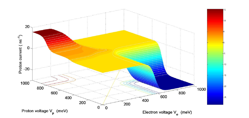
In Fig. 2, we present the numerical solution for the dependence of the proton current $I_{N}$ on the electron ($V_{e}$) and proton ($V_{p}$) voltages at the physiological temperature $T=36.6^{\circ}$C, with $E_{2}=850$ meV. The particle current is measured here in the inverse nanoseconds, ${\rm ns}^{-1}$, so that, for example, the value $I_{N}=-1\ {\rm ns}^{-1}$ corresponds to the transfer of one proton per one nanosecond from the negative side of the membrane to the positive side. It is evident from Fig. 2 that the uphill proton current (corresponding to negative values of $I_{N}$) starts at electron voltages exceeding a threshold value $V_{e0}=550$ meV provided that the proton voltage build-up is less than $450$ meV. At these voltages, the states

$$|7\rangle=a_{1}^{+}b_{2}^{+}|{\rm Vac}\rangle\ \ {\rm and}\ \ |8\rangle=a_{2}^{+}b_{1}^{+}|{\rm Vac}\rangle$$

participating in the Förster transfer (see Eq. (42)) and having energies $\sim 550$ meV begin to be populated. It is of interest that at lower voltages the state $|6\rangle=a_{1}^{+}b_{1}^{+}|{\rm Vac}\rangle$ containing an electron in the state $1_{e}$ with energy $\epsilon_{1}=100$ meV and a proton in the state $1_{p}$, having an energy $E_{1}=350$ meV, is partially populated. Here, the electron-proton Coulomb attraction, $u_{11}=-400$ meV, comes into play, lowering the total energy to the value $\varepsilon_{6}=50$ meV.

For the chosen parameters, the particle current $I_{N}$ saturates at electron voltages higher than 700 meV with the value corresponding to the translocation of 30 protons in one nanosecond. It shows the efficiency of the Förster pumping mechanism, although the real rate for the proton transfer through the D-pathway (see Ref. Brand06 ) is much less: $\sim 10^{3}$ $10^{4}$ protons per second. This pumping rate can be obtained in the framework of our model if we significantly decrease the tunneling couplings between the active sites and the electron and proton reservoirs: $\Gamma_{L}\sim\Gamma_{R}\sim 10^{-7}\ {\rm meV},\ \ \Gamma_{N}\sim\Gamma_{P}\sim 10^{-8}\ {\rm meV}.$ It has no effect on the main features of the present model, and, in the following, we return to the case of the fast electron and proton delivery to the active sites.

If the electron voltage is low enough, $V_{e}<300$ meV, but the proton voltage is high, $V_{p}>500$ meV, the proton flow reverses its direction, so that the protons move along the concentration gradient from the positive side of the membrane to the mitochondria interior. The downhill flow of the protons is especially significant when the proton voltage exceeds the value of 850 meV. However, even at high proton voltages, the discharge of the mitochondrion battery can be prevented by applying the electron potential above the threshold $V_{e0}=550$ mV. We emphasize that, within this model, we do not need any additional gates to inhibit the translocation of protons back to the negatively-charged interior, although the pump can work in the reverse regime. The optimal value for the proton voltage build-up, $V_{p}=250$ meV, correlates well with experimental data for the proton-motive force of about 200–250 meV Wik04 ; Brand06 ; Papa04 .

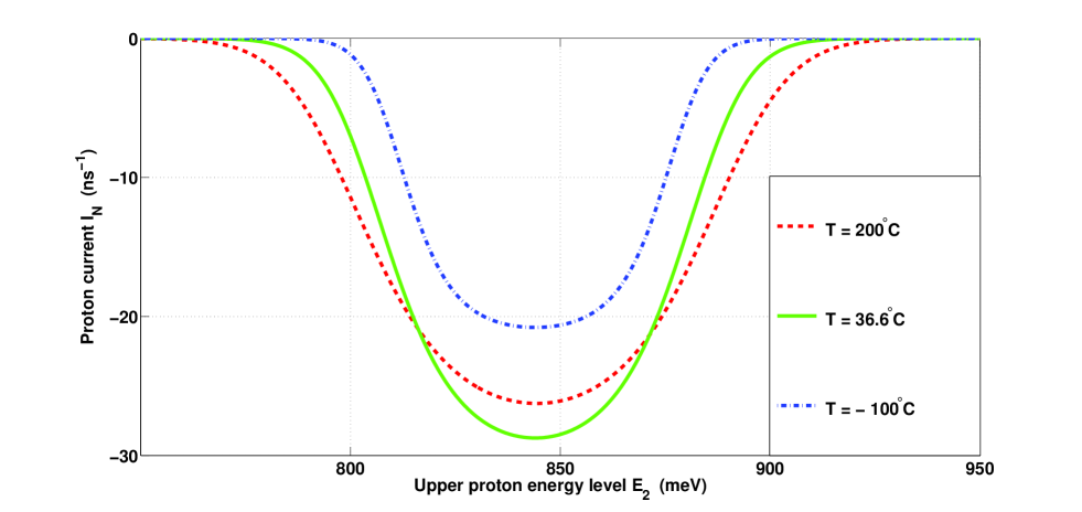
The resonant character of the Förster energy transfer is demonstrated in Fig. 3 where we plot a dependence of the proton current $I_{N}$ on the variation of the higher energy level of the protons, $E_{2}$, at several temperatures $T$ measured in degrees Celsius. It is evident that the current $I_{N}$ has the maximum absolute value at the energy

$$E_{2}=\epsilon_{2}-\epsilon_{1}+E_{1}-\lambda=844\ {\rm meV},$$

which is slightly shifted from its resonance value $E_{2}=850$ meV in accordance with the maximum of the Marcus constant $\kappa$, Eq. (43).

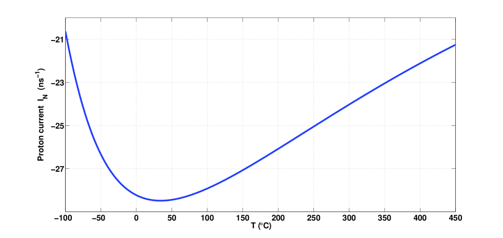
In Fig. 4 we present the temperature dependence of the uphill proton current near the optimal point

$$V_{e}\,=\,700\ {\rm meV},\;V_{p}\,=\,250\ {\rm meV},\;E_{2}=850\ {\rm meV}.$$

It is clear that the proton pumping peaks at temperatures between $0^{\circ}$C and $100^{\circ}$C with a strong decrease when the environment is colder than the water freezing point $0^{\circ}$C. However, the effect survives much better at high temperatures. Curiously, for the parameters used the uphill proton current has a maximum at temperatures about that of the human body $(36.6^{\circ}$C).

VI Conclusions

In conclusion, we proposed and analyzed quantitatively a simple nano-electronic and nano-protonic model reflecting the main features of the electron-driven proton pump in the enzyme cytochrome c oxidase. We analyzed quantum-mechanical Hamiltonians for this system taking into account tunneling couplings of electrons and protons to their corresponding reservoirs and dissipative environments, as well as the electron-proton Coulomb interaction, including the resonant Förster term. Applying methods of condensed matter physics, we obtained expressions for the electron and proton currents as well as the equations of motion for the density matrix of the system. These equations were solved numerically, and we demonstrated that the resonant Förster energy exchange between electrons and protons can lead to the proton transfer from the region with smaller proton concentration to the region with larger proton concentration, thereby achieving a proton pump. The dependence of this phenomenon on temperature and the system parameters were studied and we showed that the proton pump works with maximum efficiency near physiological temperatures and at electron and proton voltage build-ups related to their values for living cells.

Acknowledgements

This work was supported in part by the National Security Agency, Laboratory of Physical Sciences, Army Research Office, National Science Foundation grant No. EIA-0130383, and JSPS CTC Program. L.M. is partially supported by the NSF NIRT, grant ECS-0609146.

References

  • (1) B. Alberts,  A. Johnson,  J. Lewis,  M. Raff, K. Roberts, and P. Walter,  Molecular Biology of the Cell (Garland Science, New York, 2002), Ch. 11 and Ch. 14.
  • (2) M. Wikström, Biochem. Biophys. Acta 1655, 241 (2004).
  • (3) G. Bränden,  R.B. Gennis, and P. Brzezinski, Biochim. Biophys. Acta 1757, 1052 (2006).
  • (4) I. Belevich, D. A. Bloch, N. Belevich, M. Wikström, and M.I. Verkhovsky, Proc. Nat. Acad. Sci. 104, 2685 (2007).
  • (5) M. Wikström and M.I. Verkhovsky, Biochim. Biophys. Acta, in press (2007).
  • (6) S. Papa, N. Capitanio, and G. Capitanio, Biochem. Biophys. Acta 1655, 353 (2004).
  • (7) D. Bloch, I. Belevich, A. Jasaitis, C. Ribacka, A. Puustinen, M.I. Verkhovsky, and M. Wikström, Proc. Nat. Acad. Sci. 101, 529 (2004).
  • (8) J. Quenneville, D. M. Popovic, and A. A. Stuchebrukhov, Biochem. Biophys. Acta 1757, 1035 (2006).
  • (9) M. Wikström and M.I. Verkhovsky, Biochem. Biophys. Acta 1757, 1047 (2006).
  • (10) I. Belevich, M.I. Verkhovsky, and M. M. Wikström, Nature 440, 829 (2006).
  • (11) P.E.M. Siegbahn, M.R.A. Blomberg, and M.L. Blomberg, J. Phys.Chem. B 107, 10946 (2003).
  • (12) M.R.A. Blomberg and P.E.M. Siegbahn, Biochim. Biophys. Acta 1757, 969 (2006).
  • (13) P.E.M. Siegbahn and M.R.A. Blomberg, Biochim. Biophys. Acta 1767, 1143 (2007).
  • (14) M.H.M. Olsson, P.E.M. Siegbahn, M.R.A. Blomberg, and A. Warshel, Biochem. Biophys. Acta 1767, 244 (2007).
  • (15) J.P. Hosler, S. Ferguson-Miller, and D. A. Mills, Annu. Rev. Biochem. 75, 165 (2006).
  • (16) N.S. Wingreen, A.-P. Jauho, and Y. Meir, Phys. Rev. B 48, 8487 (1993); N.S. Wingreen and Y. Meir, Phys. Rev. B 49, 11040 (1994).
  • (17) T. Förster, Annalen der Physik 2, 55 (1948).
  • (18) A. Ishijima and T. Yanagida, Trends in Biochem. Sciences 26, 438 (2001); I. L. Mednitz, A.R. Clapp, H. Mattoussi, E.R. Goldman, B. Fisher, and J.M. Mauro, Nature Materials 2, 630 (2003); J. Gilmore and R.H. McKenzie, J. Phys.: Cond. Matter 17, 1735 (2005); D.W. Piston and G.-J. Kremers, Trends in Biochem. Sciences 32, 407 (2007).
  • (19) M. Achermann, M.A. Petruska, S. Kos, D.L. Smith, D.D. Koleske, and V.I. Klimov, Nature 429, 642 (2004).
  • (20) A.O. Govorov, Phys. Rev. B 71, 155323 (2005).
  • (21) H. Michel, Proc. Nat. Acad. Sci. 95, 12819 (1998).
  • (22) A. Garg, J. N. Onuchic, and V. Ambegaokar, J. Chem. Phys. 83, 4491 (1985).
  • (23) D. A. Cherepanov, L.I. Krishtalik, and A. Y. Mulkidjanian, Biophys. J. 80, 1033 (2001).
  • (24) R.A. Marcus and N. Sutin, Biochim. Biophys. Acta 811, 265 (1985).
Refer to caption
Figure 1: (Color online) (a) Schematic diagram of the electron and proton pathways in cytochrome $c$ oxidase with suggested locations for the active electron and proton sites. (b) Schematic energy diagram of the simultaneous electron and proton transport.
Refer to caption
Figure 2: (Color online) Proton current $I_{N}$ (a number of protons transferred through the membrane in one nanosecond) as a function of the electron $(V_{e})$ and proton $(V_{p})$ voltage build-ups at the physiological temperature $T=36.6^{\circ}$C and at the resonant condition, $E_{2}=850$ meV. Notice that the absolute value of the electron charge, $|e|$, is included into the definitions of voltages $V_{e},~{}V_{p}$, which are measured here in meV.
Refer to caption
Figure 3: (Color online) Dependence of the proton current $I_{N}$ on the resonant conditions (a variation of the upper proton energy level $E_{2}$) at different temperatures, for optimal values of the electron and proton voltages: $V_{e}=700$ meV, $V_{p}=250$ meV.
Refer to caption
Figure 4: Proton current $I_{N}$ as a function of temperature $T$ for $E_{2}=850$ meV, $V_{e}=700$ meV, $V_{p}=250$ meV. The maximum value of the uphill proton current $|I_{N}|$ (which appears as a minimum in the plot) corresponds to the temperature $T=36.6^{\circ}$C.