How does Casimir energy fall? III. Inertial forces on vacuum energy.

Abstract

We have recently demonstrated that Casimir energy due to parallel plates, including its divergent parts, falls like conventional mass in a weak gravitational field. The divergent parts were suitably interpreted as renormalizing the bare masses of the plates. Here we corroborate our result regarding the inertial nature of Casimir energy by calculating the centripetal force on a Casimir apparatus rotating with constant angular speed. We show that the centripetal force is independent of the orientation of the Casimir apparatus in a frame whose origin is at the center of inertia of the apparatus.

1 Introduction

Two uncharged parallel conducting plates attract. Casimir in 1948 [1] demonstrated that this force of attraction can be attributed to the quantum vacuum energy associated with the electromagnetic field between the conducting plates. Precision measurement of this force since 1997 [2] being invoked as an evidence of zero-point energy of the vacuum has been questioned in [3]. The controversy arises due to the presence of divergences which make it difficult to extract self energies for single bodies. The local energy density, a component of the stress tensor, serves as a source to gravity. Surface divergences in the local energy densities cause a serious difficulty in attempts to understand how the vacuum energy interacts with gravity.

In Fall I [4] we demonstrated, using variational principles, that the gravitational force on Casimir energy is the same as that on a conventional mass. In Fall II [5] we considered the motion of a Casimir apparatus undergoing a constant acceleration. The Casimir apparatus consisted of semi-transparent parallel plates, realized by background fields consisting of delta function potentials, which induced boundary conditions on a massless scalar field. The motion of the apparatus was studied in the accelerated frame of reference, described by Rindler coordinates, in which it experiences a pseudo-force. This fictitious force is equated to the gravitational force by the principle of equivalence. We concluded that Casimir energy, including the divergent contributions, falls under gravity like conventional mass. We made the remarkable observation that the divergent contributions to Casimir energy could be suitably interpreted as renormalizing the bare masses of the individual Casimir plates. Saharian et al. [6], using zeta function technique for regularization, earlier reached at a similar conclusion for the finite part of the Casimir energy. Thus, in Fall I and II, which has been summarized and submitted to this proceedings by K A Milton [7], we have convincingly demonstrated that Casimir energy falls like conventional mass in a weak gravitational field.

To further verify our conclusion we here study the centripetal force acting on a rotating Casimir apparatus. Firstly, we use this opportunity to refine our definition of the force on the energy associated with the field. Next, we consider a Casimir apparatus rotating with constant angular speed such that the surfaces of the plates remain parallel to the tangent to the circle of rotation. We use appropriate curvilinear coordinates to transform into the accelerated frame of reference. We demonstrate that, exactly as in the case of Rindler acceleration, the Casimir energy, including its divergent parts, experiences a centripetal force exactly like a conventional mass. We express the centripetal acceleration in terms of the center of inertia of the apparatus. Finally, we consider a rotating Casimir apparatus such that the plates makes an arbitrary angle with respect to the tangent to the circle. We demonstrate that the centripetal force is independent of the orientation of the Casimir apparatus in a frame in which the center of inertia evaluates to zero.

2 Force in the local Lorentz coordinates

Consider the curvilinear coordinates $x^{\mu}\equiv(t,x,y,z)$ with the associated metric $g_{\mu\nu}(x)$. A particular set of coordinates $\bar{x}^{a}\equiv(\bar{t},\bar{x},\bar{y},\bar{z})$ with metric $\eta_{ab}=(-1,+1,+1,+1)$ are called the local Lorentz coordinates. Let us consider a transformation $\bar{x}^{a}=\bar{x}^{a}(x)$ which can always be defined in a local neighbourhood. Any spatial point ${\bf x}$ in the curvilinear coordinates is called a point of reference [8]. As a warm-up, and to acquaint ourselves with the notations, let us define the velocity of the point of reference ${\bf x}$ as measured in the local Lorentz coordinates at time $\bar{t}$. To this regard we can write

$$\Delta{\bf\bar{x}} =\Delta{x^{i}}\frac{\partial{\bf\bar{x}}}{\partial x^{i}}+\Delta t\frac{\partial{\bf\bar{x}}}{\partial t},\qquad\qquad\Delta\bar{t} =\Delta{x^{i}}\frac{\partial\bar{t}}{\partial x^{i}}+\Delta t\frac{\partial\bar{t}}{\partial t},$$ (1)

in terms of which the velocity of the point of reference ${\bf x}$ as measured in the local Lorentz coordinates at time $\bar{t}$ will be

$${\bf v}({\bf\bar{x}},\bar{t})=\left.\frac{\Delta{\bf\bar{x}}}{\Delta\bar{t}}\right|_{\bf x}=\left[\frac{\partial\bar{t}(x)}{\partial t}\right]^{-1}\frac{\partial{\bf\bar{x}}(x)}{\partial t},$$ (2)

because $\Delta{x^{i}}=0$ for the point of reference.

A specific field, which is an analog of a fluid, is described by the corresponding energy-momentum tensor $t_{\mu\nu}(x)$. The momentum of a small volume containing the field at a point of reference ${\bf x}$ as measured in the local Lorentz coordinates at time $\bar{t}$ is

$$\bar{P}^{a}(\bar{x})=d\Sigma_{b}(\bar{x})\,t^{ab}(\bar{x})=d\Sigma_{\nu}(x)\,t^{\mu\nu}(x)\,\frac{\partial\bar{x}^{a}(x)}{\partial x^{\mu}}=P^{\mu}(x)\frac{\partial\bar{x}^{a}(x)}{\partial x^{\mu}},$$ (3)

where we have used tensor transformation properties. The spatial volume elements are constructed as the antisymmetric product of three space like vectors, $d\Sigma_{a}(\bar{x})=\epsilon_{abcd}\,\delta_{1}\bar{x}^{b}\,\delta_{2}\bar{x}^{c}\,\delta_{3}\bar{x}^{d}$, and $d\Sigma_{\mu}(x)=\sqrt{-g(x)}\,\epsilon_{\mu\nu\alpha\beta}\,\delta_{1}x^{\nu}\,\delta_{2}x^{\alpha}\,\delta_{3}x^{\beta}$, where $g(x)=\mbox{det}\,g_{\mu\nu}(x)$. The change in momentum when the coordinates are displaced will be

$$\Delta\bar{P}^{a}(\bar{x})=\Delta\bar{x}^{i}\frac{\partial}{\partial\bar{x}^{i}}\bar{P}^{a}(\bar{x})+\Delta\bar{t}\frac{\partial}{\partial\bar{t}}\bar{P}^{a}(\bar{x})$$ (4)

and the force density as measured in the local Lorentz coordinates at time $\bar{t}$ is

$$\bar{F}^{a}(\bar{x})=\left.\frac{\Delta\bar{P}^{a}}{\Delta\bar{t}}\right|_{\bf x} = \left.\frac{\Delta\bar{x}^{i}}{\Delta\bar{t}}\right|_{\bf x}\left.\frac{\partial}{\partial\bar{x}^{i}}\bar{P}^{a}(\bar{x})\right|_{\bf x}+\left.\frac{\partial}{\partial\bar{t}}\bar{P}^{a}(\bar{x})\right|_{\bf x}$$ (5)

$$= \left[\frac{\partial\bar{t}(x)}{\partial t}\right]^{-1}\left[\frac{\partial}{\partial t}\bar{P}^{a}(\bar{x})\right]_{\bf x}$$

$$= \left[\frac{\partial\bar{t}(x)}{\partial t}\right]^{-1}\frac{\partial}{\partial t}\left[P^{\mu}(x)\frac{\partial\bar{x}^{a}(x)}{\partial x^{\mu}}\right],$$

where we used (2) in going from first line to the second line.

The total force on the energy associated with the field as measured in the local Lorentz coordinates at time $\bar{t}$ is obtained by integrating the force density over a surface $S$ described by constant $\bar{t}$. Thus

$$\bar{F}^{a}(\bar{t}) = \int_{S}\left[\frac{\partial\bar{t}(x)}{\partial t}\right]^{-1}\frac{\partial}{\partial t}\left[P^{\mu}(x)\frac{\partial\bar{x}^{a}(x)}{\partial x^{\mu}}\right]$$ (6)

$$= \int d^{3}x\left[\frac{\partial\bar{t}(x)}{\partial t}\right]^{-1}\,\frac{\partial}{\partial t}\left[\sqrt{-g(x)}\,t^{\mu 0}(x)\,\frac{\partial\bar{x}^{a}(x)}{\partial x^{\mu}}\right].$$

This probably is rigorously true only for situations when the field under consideration is sufficiently localized and thus requires scrutiny. In the special case when both the metric tensor and the energy momentum tensor are independent of the coordinate time $t$ the above expression takes the simpler form

$$\bar{F}^{a}(\bar{t}) = \int d^{3}x\sqrt{-g(x)}\,t^{\mu 0}(x)\,\left[\frac{\partial}{\partial t}\,\frac{\partial\bar{x}^{a}(x)}{\partial x^{\mu}}\right]\left[\frac{\partial\bar{t}(x)}{\partial t}\right]^{-1}.$$ (7)

2.1 Rindler metric

As an illustrative example let us reconsider the situation in Fall II using the above definition. The local Lorentz coordinates $\bar{x}^{a}$ are related to the Rindler coordinates $x^{\mu}\equiv(\tau,x,y,\xi)$ by the transformations: $\bar{t}=\xi\sinh\tau,\;\bar{x}=x,\;\bar{y}=y,\;\bar{z}=\xi\cosh\tau$. The Rindler metric is $g_{\mu\nu}(x)=(-\xi^{2},+1,+1,+1)$ which returns $g(x)=-\xi^{2}$. Further for the Casimir apparatus considered in Fall II we have only the diagonal components of $t_{\mu\nu}(x)$ to be nonzero which are independent of $\tau$. Using these in (7) we determine the force on the vacuum energy associated with the Casimir apparatus to be

$$\frac{F^{3}}{A}=\int_{0}^{\infty}\frac{d\xi}{\xi}\,\xi^{2}\,t^{00}(\xi)=\int_{0}^{\infty}\frac{d\xi}{\xi}\,\frac{1}{\xi^{2}}\,t_{00}(\xi)=-\int_{0}^{\infty}\frac{d\xi}{\xi}\,{t^{0}}_{0}(\xi),$$ (8)

which leads to the result in Fall II

$$F^{3}=\left[E_{\rm a}^{(0)}+E_{\rm b}^{(0)}+E_{\rm cas}^{(0)}\right]g,$$ (9)

where the first two terms are the divergent energies associated with the individual plates and $E_{\rm cas}^{(0)}$ is the Casimir energy. Further, using the stress tensor for a conventional mass,

$$t^{\mu\nu}(x)=m_{\rm a}\frac{1}{\sqrt{-g(x)}}\int_{-\infty}^{+\infty}ds\,\delta^{(4)}(x-x_{\rm a}(s))\frac{dx^{\mu}}{ds}\frac{dx^{\nu}}{ds},$$ (10)

in (8) we have the force on the plates to be

$$F^{3}=\left[m_{\rm a}+m_{\rm b}\right]g.$$ (11)

Thus, the total force on the Casimir apparatus, including the sum of the force on the vacuum energy, and the plates, is

$$F^{3}=\left[m_{\rm a}+m_{\rm b}+E_{\rm a}^{(0)}+E_{\rm b}^{(0)}+E_{\rm cas}^{(0)}\right]g.$$ (12)

Interpreting $m_{\rm a,b}$ to be the bare masses of the plates and renormalizing $m_{\rm a,b}+E_{\rm a,b}^{(0)}\rightarrow M_{\rm a,b}$ we thus conclude

$$F^{3}=\left[M_{\rm a}+M_{\rm b}+E_{\rm cas}^{(0)}\right]g,$$ (13)

where $M_{a,b}$ are the renormalized masses of the plates.

3 Rotating Casimir apparatus

A scalar field $\bar{\phi}(\bar{x})$ in the presence of a background $\bar{V}(\bar{x})$ is described by the action

$$W=\int d^{4}\bar{x}\left[-\frac{1}{2}\eta^{ab}\bar{\partial}_{a}\bar{\phi}(\bar{x})\bar{\partial}_{b}\bar{\phi}(\bar{x})-\frac{1}{2}\bar{V}(\bar{x})\bar{\phi}(\bar{x})^{2}\right].$$ (14)

A Casimir apparatus, built out of so-called semi-transparent plates, rotating with constant angular speed $\omega$ about the $\bar{x}$ axis, as illustrated in figure 1, will be described by the potential

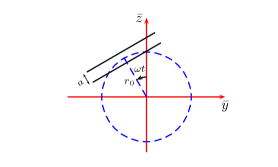
Figure 1: Casimir apparatus rotating with constant angular speed $\omega$ about the $\bar{x}$ axis. The plane of the plates are chosen to be perpendicular to the radial direction. We have $r_{a}=r_{0}-\frac{a}{2}$, and $r_{b}=r_{0}+\frac{a}{2}$.

$$\bar{V}(\bar{x}) = \lambda_{a}\,\delta(\bar{z}\cos\omega\bar{t}-\bar{y}\sin\omega\bar{t}-r_{a})+\lambda_{b}\,\delta(\bar{z}\cos\omega\bar{t}-\bar{y}\sin\omega\bar{t}-r_{b})$$ (15a)

$$= \lambda_{a}\,\delta\left(\bar{z}\cos\omega\bar{t}-\bar{y}\sin\omega\bar{t}-r_{0}+\frac{a}{2}\right)+\lambda_{b}\,\delta\left(\bar{z}\cos\omega\bar{t}-\bar{y}\sin\omega\bar{t}-r_{0}-\frac{a}{2}\right).$$ (15b)

Making the following transformations

$$y =+\bar{y}\cos\omega\bar{t}+\bar{z}\sin\omega\bar{t},\qquad\qquad x=\bar{x},$$ (15pa)

$$z =-\bar{y}\sin\omega\bar{t}+\bar{z}\cos\omega\bar{t}-r_{0},\qquad\qquad t=\bar{t},$$ (15pb)

which has the following inverse transformations

$$\bar{y} =y\cos\omega t-(z+r_{0})\sin\omega t,\qquad\qquad \bar{x}=x,$$ (15pqa)

$$\bar{z} =y\sin\omega t+(z+r_{0})\cos\omega t,\qquad\qquad \bar{t}=t,$$ (15pqb)

the action in (14) takes the form

$$W=\int d^{4}x\sqrt{-g(x)}\,{\cal{L}}(\phi(x)),$$ (15pqr)

where

$${\cal{L}}(\phi(x))=-\frac{1}{2}g^{\mu\nu}(x)\partial_{\mu}\phi(x)\partial_{\nu}\phi(x)-\frac{1}{2}V(x)\phi(x)^{2},$$ (15pqs)

in which the background potential,

$$V(x)=\lambda_{a}\,\delta\left(z+\frac{a}{2}\right)+\lambda_{b}\,\delta\left(z-\frac{a}{2}\right),$$ (15pqt)

is now independent of $t$. The metric is

$$g_{\mu\nu}(x)=\left[\begin{array}[]{cccc}-(1-\omega^{2}r^{2})&0&-\omega(z+r_{0})&\omega y\\ 0&1&0&0\\ -\omega(z+r_{0})&0&1&0\\ \omega y&0&0&1\end{array}\right],$$ (15pqu)

and its inverse is

$$g^{\mu\nu}(x)=\left[\begin{array}[]{cccc}-1&0&-\omega(z+r_{0})&\omega y\\ 0&1&0&0\\ -\omega(z+r_{0})&0&\{1-\omega^{2}(z+r_{0})^{2}\}&\omega^{2}y(z+r_{0})\\ \omega y&0&\omega^{2}y(z+r_{0})&(1-\omega^{2}y^{2})\end{array}\right],$$ (15pqv)

where $r^{2}=y^{2}+(z+r_{0})^{2}$, and $g(x)={\rm det}\,g_{\mu\nu}(x)=-1$. For the sake of bookkeeping we note the corresponding nonzero components of the connection symbols: $\Gamma^{2}_{00}=-\omega^{2}y,\Gamma^{3}_{00}=-\omega^{2}z$, and $\Gamma^{3}_{02}=-\Gamma^{2}_{03}=\omega$. The energy-momentum tensor, or the stress tensor, in the curvilinear coordinates is

$$t_{\alpha\beta}(x)=\partial_{\alpha}\phi(x)\partial_{\beta}\phi(x)+g_{\alpha\beta}(x){\cal{L}}(\phi(x)).$$ (15pqw)

At the one-loop level the Green’s function $G(x,x^{\prime})$ is related to the fields by the correspondence $\langle T\phi(x)\phi(x^{\prime})\rangle=-\rmi\,G(x,x^{\prime})$.

3.1 Centripetal force

In terms of the curvilinear coordinates the potential (15pqt) is independent of time $t$ which renders the energy-momentum tensor independent of time. Using this in (7) we calculate the force on the vacuum energy associated with the Casimir apparatus to be

$$\bar{F}^{a}(\bar{t})=\int d^{3}x\,t^{\mu 0}(x)\,\frac{\partial}{\partial t}\frac{\partial\bar{x}^{a}(x)}{\partial x^{\mu}}.$$ (15pqx)

We shall be interested in the leading order contributions to the force in the parameter $\omega r_{0}$. To this end we observe that only the zeroth order term in the energy-momentum tensor contributes, which is diagonal and a function of $z$ alone. Using this in (15pqx) we can write the centripetal force on the vacuum energy to be

$$\bar{\bf F}(\bar{t})=-\omega^{2}\,\hat{\bar{\bf r}}(\omega\bar{t})\,r_{0}\int d^{3}x\,t_{00}^{(0)}(z)-\omega^{2}\,\hat{\bar{\bf r}}(\omega\bar{t})\int d^{3}x\,z\,t_{00}^{(0)}(z)+\omega^{2}{\cal O}(\omega r_{0}),$$ (15pqy)

where the unit vector is $\hat{\bar{\bf r}}(\theta)=\cos\theta\,\hat{\bar{\bf z}}-\sin\theta\,\hat{\bar{\bf y}}$. We define the total energy associated with the field and the center of inertia (energy) as measured in the curvilinear coordinates as

$$E^{(0)}_{\rm tot}=\int d^{3}x\,t_{00}^{(0)}(x)\qquad{\rm and}\qquad z_{\rm cm}=\frac{1}{E^{(0)}_{\rm tot}}\int d^{3}x\,z\,t_{00}^{(0)}(x)$$ (15pqz)

respectively, in terms of which the centripetal force in (15pqy) can be written in the form

$$\bar{\bf F}(\bar{t})=-\omega^{2}\,\left[r_{0}+z_{\rm cm}\right]\,\hat{\bar{\bf r}}(\omega\bar{t})\,E_{\rm tot}^{(0)}=-\omega^{2}\,\bar{r}_{\rm cm}\,\hat{\bar{\bf r}}(\omega\bar{t})\,E_{\rm tot}^{(0)},$$ (15pqaa)

where $\bar{r}_{\rm cm}=r_{0}+z_{\rm cm}$, is the center of inertia in the local Lorentz coordinates. $t_{00}^{(0)}(z)$ is the energy density of the plates when the acceleration is switched off. In particular we recall

$$t_{00}^{(0)}(x)=\frac{1}{2\rmi}\left\{\left(\frac{\partial}{\partial t}\frac{\partial}{\partial t^{\prime}}-\frac{\partial^{2}}{\partial t^{2}}\right)G^{(0)}(x,x^{\prime})\right\}_{x=x^{\prime}}+\,\frac{1}{4\rmi}\,{\nabla}^{2}G^{(0)}(x,x),$$

where the Green’s function is of the form

$$G^{(0)}(x,x^{\prime})=\int_{-\infty}^{+\infty}\frac{d\omega}{2\pi}\int\frac{d^{2}k_{\perp}}{(2\pi)^{2}}\,e^{-\rmi\omega(t-t^{\prime})}e^{\rmi{\bf k}_{\perp}\cdot({\bf x}_{\perp}-{\bf x}_{\perp}^{\prime})}g^{(0)}(z,z^{\prime};\kappa),$$

with $\kappa^{2}={\bf k}_{\perp}^{2}-\omega^{2}$, and $g^{(0)}(z,z^{\prime};\kappa)$ satisfies

$$-\left[\frac{\partial^{2}}{\partial z^{2}}-\kappa^{2}-V^{(0)}(z)\right]g^{(0)}(z,z^{\prime};\kappa)=\delta(z-z^{\prime}).$$ (15pqab)

Using these relations the total energy per unit area in (15pqz) takes the form

$$\frac{E^{(0)}_{\rm tot}}{A}=-\frac{1}{2}\int_{-\infty}^{+\infty}\frac{d\zeta}{2\pi}\int\frac{d^{2}k_{\perp}}{(2\pi)^{2}}\,2\zeta^{2}\int_{-\infty}^{+\infty}dz\,g^{(0)}(z,z;\kappa),$$ (15pqac)

where we have switched to imaginary frequencies, $\omega\rightarrow\rmi\zeta$, thus $\kappa^{2}={\bf k}_{\perp}^{2}+\zeta^{2}$. Center of inertia in (15pqz) can be similarly expressed in terms of the first moment of $g^{(0)}(z,z;\kappa)$.

3.2 Centripetal force on a single plate

A single plate rotating with constant angular speed is described by a single delta function in the potential in (15pqt) (letting $a=0$, $r_{0}=r_{a}$, and $\lambda_{b}=0$),

$$V(z)=\lambda_{a}\,\delta(z),$$ (15pqad)

and the corresponding solution to eq. (15pqab) evaluated at $z=z^{\prime}$ is

$$g^{(0)}(z,z;\kappa)=\frac{1}{2\kappa}-\frac{\lambda_{a}}{\lambda_{a}+2\kappa}\frac{1}{2\kappa}\,e^{-2\kappa|z|}$$ (15pqae)

in terms of which the force in (15pqaa) evaluates to

$$\bar{\bf F}(\bar{t})=-\hat{\bar{\bf r}}(\omega\bar{t})\,\omega^{2}\bar{r}_{\rm cm}\,E_{a}^{(0)},$$ (15pqaf)

where $\bar{r}_{\rm cm}=r_{0}=r_{a}$, and

$$\frac{E_{a}^{(0)}}{A}=\frac{1}{12\pi^{2}}\int_{0}^{\infty}\kappa^{2}d\kappa\,\frac{\lambda_{a}}{\lambda_{a}+2\kappa}=\frac{1}{96\pi^{2}}\int_{0}^{\infty}\frac{dy}{y}\,\frac{y^{3}}{1+\frac{y}{\lambda_{a}}},$$ (15pqag)

a divergent quantity, is the energy per unit area associated with a single plate. The center of inertia, $z_{\rm cm}$, in (15pqz) evaluates to zero for a single plate.

3.3 Parallel plates

Two parallel plates separated by a distance $a$ and rotating with constant angular speed $\omega$ is described by the potential in (15pqt). The reduced Green’s function, $g^{(0)}(z,z^{\prime};\kappa)$, which is solution to (15pqab), evaluated at $z=z^{\prime}$, in the region $z<-\frac{a}{2}$ is

$$\frac{1}{2\kappa}-\frac{1}{2\kappa}\frac{e^{2\kappa z}}{\Delta}\left[\frac{\lambda_{a}}{2\kappa}\left(1+\frac{\lambda_{b}}{2\kappa}\right)e^{\kappa a}+\frac{\lambda_{b}}{2\kappa}\left(1-\frac{\lambda_{a}}{2\kappa}\right)e^{-\kappa a}\right],$$ (15pqah)

in the region $-\frac{a}{2}<z<\frac{a}{2}$ is

$$\frac{1}{2\kappa}-\frac{1}{2\kappa}\frac{e^{-\kappa a}}{\Delta}\left[\frac{\lambda_{a}}{2\kappa}\left(1+\frac{\lambda_{b}}{2\kappa}\right)e^{-2\kappa z}+\frac{\lambda_{b}}{2\kappa}\left(1+\frac{\lambda_{a}}{2\kappa}\right)e^{2\kappa z}-2\frac{\lambda_{a}}{2\kappa}\frac{\lambda_{b}}{2\kappa}\,e^{-\kappa a}\right],$$ (15pqai)

and in the region $\frac{a}{2}<z$ is

$$\frac{1}{2\kappa}-\frac{1}{2\kappa}\frac{e^{-2\kappa z}}{\Delta}\left[\frac{\lambda_{a}}{2\kappa}\left(1-\frac{\lambda_{b}}{2\kappa}\right)e^{-\kappa a}+\frac{\lambda_{b}}{2\kappa}\left(1+\frac{\lambda_{a}}{2\kappa}\right)e^{\kappa a}\right],$$ (15pqaj)

where

$$\Delta=\left(1+\frac{\lambda_{a}}{2\kappa}\right)\left(1+\frac{\lambda_{b}}{2\kappa}\right)-\frac{\lambda_{a}}{2\kappa}\frac{\lambda_{b}}{2\kappa}\,e^{-2\kappa a}.$$ (15pqak)

Using the above expressions for $g^{(0)}(z,z;\kappa)$ in the appropriate regions of the $z$ integral in (15pqac) the centripetal force in (15pqaa) evaluates to

$$\bar{\bf F}(\bar{t})=-\hat{\bar{\bf r}}(\omega\bar{t})\,\omega^{2}\bar{r}_{\rm cm}\left[E_{\rm a}^{(0)}+E_{\rm b}^{(0)}+E_{\rm cas}^{(0)}\right],$$ (15pqal)

where $E^{(0)}_{\rm a,b}$ are the total energies due to single plates given in terms of (15pqag), $E^{(0)}_{\rm cas}$ is the Casimir energy given as

$$\frac{E_{\rm cas}^{(0)}}{A}=-\frac{1}{12\pi^{2}}\int_{0}^{\infty}\kappa^{2}\,d\kappa\left[2\kappa a+\frac{1}{1+\frac{\lambda_{a}}{2\kappa}}+\frac{1}{1+\frac{\lambda_{b}}{2\kappa}}\right]\frac{1}{2\kappa}\frac{\partial}{\partial a}\ln\Delta,$$ (15pqam)

and $\bar{r}_{\rm cm}=r_{0}+z_{\rm cm}$, where the center of inertia in the curvilinear coordinates, $z_{\rm cm}$, for parallel plates evaluates to

$$z_{\rm cm}\,E_{\rm tot}^{(0)}=-\frac{a}{24\pi^{2}}\int_{0}^{\infty}\kappa^{2}d\kappa\frac{1}{\Delta}\left[\frac{\lambda_{b}}{2\kappa}-\frac{\lambda_{a}}{2\kappa}\right],$$ (15pqan)

which is in general not zero because of the asymmetry in the couplings, but evaluates to zero when $\lambda_{a}=\lambda_{b}$, or in the Dirichlet limit.

4 Orientation independence of centripetal force

A Casimir apparatus making an arbitrary angle $\alpha$ with respect to the tangent while rotating with constant angular speed $\omega$, as illustrated in figure 2, is described by the potential, (displaying only for one plate to save typographic space,)

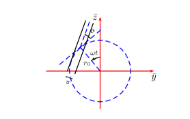
Figure 2: A Casimir apparatus oriented at an angle $\alpha$ with respect to the tangent to the circle of radius $r_{0}$ and rotating with constant angular speed $\omega$ about the $\bar{x}$ axis. We have $r_{a}\cos\alpha=r_{0}\cos\alpha-\frac{a}{2}$, $r_{b}\cos\alpha=r_{0}\cos\alpha+\frac{a}{2}$, $r_{0}=(r_{a}+r_{b})/2$, and $a=(r_{b}-r_{a})\cos\alpha$.

$$\bar{V}(\bar{x}) = \lambda_{a}\,\delta(\bar{z}\cos(\alpha+\omega\bar{t})-\bar{y}\sin(\alpha+\omega\bar{t})-r_{a}\cos\alpha)$$ (15pqaoa)

$$= \lambda_{a}\,\delta\left(\bar{z}\cos(\alpha+\omega\bar{t})-\bar{y}\sin(\alpha+\omega\bar{t})-r_{0}\cos\alpha+\frac{a}{2}\right).$$ (15pqaob)

We make the transformations

$$y =+\bar{y}\cos(\alpha+\omega\bar{t})+\bar{z}\sin(\alpha+\omega\bar{t})-r_{0}\sin\alpha,\qquad x =\bar{x},$$ (15pqaoapa)

$$z =-\bar{y}\sin(\alpha+\omega\bar{t})+\bar{z}\cos(\alpha+\omega\bar{t})-r_{0}\cos\alpha,\qquad t =\bar{t},$$ (15pqaoapb)

which has the inverse transformations

$$\bar{y} =(y+r_{0}\sin\alpha)\cos(\alpha+\omega\bar{t})-(z+r_{0}\cos\alpha)\sin(\alpha+\omega\bar{t}),\qquad\bar{x} =x,$$ (15pqaoapaqa)

$$\bar{z} =(y+r_{0}\sin\alpha)\sin(\alpha+\omega\bar{t})+(z+r_{0}\cos\alpha)\cos(\alpha+\omega\bar{t}),\qquad\bar{t} =t,$$ (15pqaoapaqb)

which reduces to the transformations in (15pa) and (15pb) for $\alpha=0$. The metric corresponding to this transformation evaluates to be

$$g_{\mu\nu}(x)=\left[\begin{array}[]{cccc}-(1-\omega^{2}r^{2})&0&-\omega(z+r_{0}\cos\alpha)&\omega(y+r_{0}\sin\alpha)\\ 0&1&0&0\\ -\omega(z+r_{0}\cos\alpha)&0&1&0\\ +\omega(y+r_{0}\sin\alpha)&0&0&1\end{array}\right],$$ (15pqaoapaqar)

where $r^{2}=(y+r_{0}\sin\alpha)^{2}+(z+r_{0}\cos\alpha)^{2}$, and reduces to the metric in (15pqu) for $\alpha=0$. Thus on, repeating the steps in section 3, we evaluate the centripetal force to be

$$\bar{\bf F}(\bar{t})=-\omega^{2}\,\bar{\bf r}_{\rm cm}(\omega\bar{t})\left[E_{\rm a}^{(0)}+E_{\rm b}^{(0)}+E_{\rm cas}^{(0)}\right],$$ (15pqaoapaqas)

where the center of inertia in the local Lorentz coordinates is

$$\bar{\bf r}_{\rm cm}(\omega\bar{t})=r_{0}\hat{\bar{\bf r}}(\omega\bar{t})+z_{\rm cm}\hat{\bar{\bf r}}(\alpha+\omega\bar{t}),$$ (15pqaoapaqat)

in which the center of inertia in the curvilinear coordinates, $z_{\rm cm}$, is again given using (15pqan). We observe that if the origin of the curvilinear coordinates is chosen such that $z_{\rm cm}=0$ then the centripetal force is independent of the orientation of the Casimir apparatus. We shall end by pointing to the discussion on frame dependence of center of mass in page 176 of reference [8] and to the original work cited in it.

References

References

• [1] H. B. G. Casimir, Kon. Ned. Akad. Wetensch. Proc.  51 (1948) 793.
• [2] S. K. Lamoreaux, Phys. Rev. Lett.  78 (1997) 5.
• [3] R. L. Jaffe, Phys. Rev.  D 72 (2005) 021301 [arXiv:hep-th/0503158].
• [4] S. A. Fulling, K. A. Milton, P. Parashar, A. Romeo, K. V. Shajesh and J. Wagner, Phys. Rev.  D 76 (2007) 025004 [arXiv:hep-th/0702091].
• [5] K. A. Milton, P. Parashar, K. V. Shajesh and J. Wagner, J. Phys. A 40 (2007) 10935 [arXiv:0705.2611 [hep-th]].
• [6] A. A. Saharian, R. S. Davtyan and A. H. Yeranyan, Phys. Rev.  D 69 (2004) 085002 [arXiv:hep-th/0307163].
• [7] K. A. Milton, S. A. Fulling, P. Parashar, A. Romeo, K. V. Shajesh and J. A. Wagner, arXiv:0710.3841 [hep-th].
• [8] C. Møller 1972 The Theory of Relativity 2nd ed (Oxford University Press, Delhi)