Towards 4-loop NSPT result for a 3-dimensional condensate-contribution to hot QCD pressure

Abstract:

Thanks to dimensional reduction, the contributions to the hot QCD pressure coming from so-called soft modes can be studied via an effective three-dimensional theory named Electrostatic QCD (spatial Yang-Mills fields plus an adjoint Higgs scalar). The poor convergence of the perturbative series within EQCD suggests to perform lattice measurements of some of the associated gluon condensates. These turn out, however, to be plagued by large discretization artifacts. We discuss how Numerical Stochastic Perturbation Theory can be exploited to determine the full lattice spacing dependence of one of these condensates up to 4-loop order, and sharpen our tools on a concrete 2-loop example.

1 Motivation

The pressure $p(T)$ of hot QCD (with a temperature $T\gg 150$ MeV) is of crucial importance in different contexts. For instance, in cosmology, the cooling rate of the Universe is given by

$$\frac{1}{T}\frac{{\rm d}T}{{\rm d}t}=-\frac{\sqrt{24\pi}}{m_{\mbox{\tiny\rm{Pl}}}}\frac{\sqrt{e(T)}s(T)}{c(T)}\;,$$ (1)

where $T$ is the temperature, $t$ the age of the Universe, $m_{\mbox{\tiny\rm{Pl}}}$ the Planck mass, and

$$s(T)=p^{\prime}(T)~{},~{}~{}~{}~{}e(T)=Ts(T)-p(T)~{},~{}~{}~{}~{}c=e^{\prime}(T)~{}.$$ (2)

On the other hand, in heavy ion collisions, the system evolves according to

$$T^{\mu\nu}\approx[p(T)+e(T)]u^{\mu}u^{\nu}-p(T)\eta^{\mu\nu}~{},~{}~{}~{}~{}\partial_{\mu}T^{\mu\nu}=0~{},$$ (3)

where $T^{\mu\nu}$ is the energy-momentum tensor, $\eta^{\mu\nu}$ the Minkowski metric, and $u^{\mu}$ the flow velocity. Finally, from a theoretical point of view, the pressure is proportional to the number of effective degrees of freedom, and is therefore a good observable to characterize hot QCD matter.

2 Theoretical setup — part I (continuum)

In general, the determination of the QCD pressure is a non-trivial task. In spite of our restriction to the deconfined phase, $T\gg 150$ MeV, where perturbation theory should in principle be applicable, it is of limited use in practice, because of the very slow convergence of the perturbative series [1]. At the same time, first principles lattice simulations are also difficult at temperatures above about $T\sim 1$ GeV [2], because the system then develops a scale hierarchy, $g^{2}T/\pi\mathop{\raise 1.29167pt\hbox{$<$\kern-7.5pt\raise-4.73611pt\hbox{$\sim$}}}gT\mathop{\raise 1.29167pt\hbox{$<$\kern-7.5pt\raise-4.73611pt\hbox{$\sim$}}}\pi T$, where $g$ is the QCD gauge coupling (for an idea to possibly overcome this limitation, see ref. [3]).

A suitable strategy to tackle the computation of $p(T)$ (and of many other observables) in this situation is given by Dimensional Reduction [4, 5, 6]: it consists of integrating out “hard modes”, with momenta $k\sim\pi T$, from the four-dimensional (4d) QCD, to arrive at an effective description in terms of so-called Electrostatic QCD (EQCD) [7], i.e. a three-dimensional (3d) Yang-Mills theory plus an adjoint Higgs field $A_{0}^{a}(x)$. The action of EQCD is given by

$$S_{\mbox{\tiny\rm{EQCD}}} = \int\!{\rm d}^{3}x\,\biggl{\{}\frac{1}{2}\mathop{\textrm{Tr}}[F_{ij}^{2}(x)]+\mathop{\textrm{Tr}}[D_{i},A_{0}(x)]^{2}+m_{\mbox{\tiny\rm{E}}}^{2}\mathop{\textrm{Tr}}[A_{0}^{2}(x)]+\lambda_{\mbox{\tiny\rm{E}}}\big{(}\mathop{\textrm{Tr}}[A_{0}^{2}(x)]~{}\!\big{)}^{2}\biggr{\}}~{},\;$$ (4)

where ${F}_{ij}^{~{}\!\!a}$ is the 3d field strength tensor; $D_{i}$ the covariant derivative; $A_{0}=\sum_{B=1}^{8}A_{0}^{B}~{}\!T^{B}$ with $\mathop{\textrm{Tr}}~{}\![T^{A}T^{B}]=\frac{1}{2}\!\delta^{AB}$; and we implicitly assume the use of dimensional regularization. The temperature $T$ now enters only via the parameters $m_{\mbox{\tiny\rm{E}}}$, $\lambda_{\mbox{\tiny\rm{E}}}$ and $g_{\mbox{\tiny\rm{E}}}$, where $g_{\mbox{\tiny\rm{E}}}$ is the EQCD gauge coupling.

It turns out that perturbation theory within EQCD might converge very slowly [7] (see, however, ref. [8]). One can then switch to a numerical measurement of the partial derivatives of the pressure with respect to the parameters of the EQCD action, the so-called condensates: after subtracting the proper counterterms, the results are extrapolated to the continuum and then numerically integrated to finally get $p(T)$ [9]. It turns out that carrying out the continuum extrapolation is difficult because of large $O(a)$ discretization effects: thanks to super-renormalizability, these effects are however purely perturbative in nature, and our aim is to determine them up to 4-loop level.

3 Theoretical setup — part II (lattice)

The EQCD action on the lattice may be written as

$$S_{\mbox{\tiny\rm{latt}}} = \beta\sum_{\mbox{\tiny\rm{$x,~{}\!i<j$}}}\Bigl{(}1-\frac{1}{3}\mathop{\rm Re}\mathop{\textrm{Tr}}\big{[}P_{ij}(x)\big{]}\Bigr{)}-$$ (5)

$$- 2\sum_{\mbox{\tiny\rm{$x,~{}\!i<j$}}}\mathop{\textrm{Tr}}\big{[}\phi(x)~{}\!U_{i}(x)~{}\!\phi(x+i)~{}\!U_{i}^{{\dagger}}(x)\big{]}+$$

$$+ \sum_{\mbox{\tiny\rm{$x$}}}\bigg{\{}\alpha(\beta,\lambda,am_{\mbox{\tiny\rm{E}}})\mathop{\textrm{Tr}}\big{[}\phi^{2}(x)\big{]}+\lambda\Big{(}\!\mathop{\textrm{Tr}}\big{[}\phi^{2}(x)\big{]}\Big{)}^{2}\bigg{\}}~{},$$

where $\beta=6/ag_{\mbox{\tiny\rm{E}}}^{2}$, $P_{ij}$ is the plaquette, $U_{i}$ is the link variable, $\phi=\sqrt{a}A_{0}$, $\lambda=a\lambda_{\mbox{\tiny\rm{E}}}$, and [10]

$$\alpha(\beta,\lambda,am_{\mbox{\tiny\rm{E}}}) = 6\bigg{\{}1+\frac{(am_{\mbox{\tiny\rm{E}}})^{2}}{6}-\bigg{(}6+\frac{5}{3}\lambda\beta\bigg{)}\frac{3.175911525625}{4\pi\beta}-$$

$$- \frac{3}{8\pi^{2}\beta^{2}}~{}\!\bigg{[}\bigg{(}10\lambda\beta-\frac{5}{9}\lambda^{2}\beta^{2}\bigg{)}\bigg{(}\ln\beta+0.08849\bigg{)}+\frac{34.768}{6}\lambda\beta+36.130\bigg{]}\bigg{\}}~{}.$$

The quantity under inspection is the derivative of $p(T)$ with respect to $(am_{\mbox{\tiny\rm{E}}})^{2}$; this yields $\langle~{}\!\!\mathop{\textrm{Tr}}~{}\!\![~{}\!\phi^{2}]~{}\!\rangle$, which can be expanded as

$$\langle~{}\!\!\mathop{\textrm{Tr}}~{}\!\![~{}\!\phi^{2}]~{}\!\rangle = d_{00}+d_{10}~{}\!\frac{1}{\beta}+d_{11}\lambda+d_{20}~{}\!\frac{1}{\beta^{2}}+d_{21}~{}\!\frac{\lambda}{\beta}+d_{22}\lambda^{2}+$$ (7)

$$+ d_{30}~{}\!\frac{1}{\beta{{}^{3}}}+d_{31}~{}\!\frac{\lambda}{\beta{{}^{2}}}+d_{32}~{}\!\frac{\lambda^{2}}{\beta}+d_{33}\lambda^{3}+{O}\bigg{(}~{}\!\frac{\lambda^{n}}{\beta{{}^{4-n}}}\bigg{)}~{}.\vspace{0.5cm}$$

The coefficients $d_{00}$, $d_{10}$, $d_{11}$, $d_{21}$ and $d_{22}$ are known analytically, for instance ($N\equiv$ lattice extent)

$$d_{11} = 40\biggl{[}\frac{3.175911525625}{4\pi}-\frac{1}{N^{3}}\sum_{n_{1}=0}^{N-1}\,\sum_{n_{2}=0}^{N-1}\,\sum_{n_{3}=0}^{N-1}\frac{1}{4\sum_{i=1}^{3}\sin^{2}(\frac{\pi n_{i}}{N})+(am_{\mbox{\tiny\rm{E}}})^{2}}\biggr{]}\times$$ (8)

$$\times \frac{1}{N^{3}}\sum_{k_{1}=0}^{N-1}\,\sum_{k_{2}=0}^{N-1}\,\sum_{k_{3}=0}^{N-1}\biggl{[}\frac{1}{4\sum_{i=1}^{3}\sin^{2}(\frac{\pi k_{i}}{N})+(am_{\mbox{\tiny\rm{E}}})^{2}}\biggr{]}^{2}\;,$$

but the others have to be determined: those with the biggest impact are expected to be the 3-loop and 4-loop coefficients independent of $\lambda$, i.e. ${d_{20}}$ and ${d_{30}}$, respectively.

4 Numerical setup

The perturbative study is concretely carried out by means of Numerical Stochastic Perturbation Theory (NSPT) [11]. (Incidentally, it would also be interesting to pursue the same computation with standard techniques [12].) Its origins lie in Stochastic Quantization [13], based on introducing an extra coordinate $t$ and an evolution equation of the Langevin type, namely

$$\partial_{t}\phi(x,t)=-\partial_{\phi}S[\phi]+\eta(x,t)~{},$$ (9)

where $\eta(x,t)$ is a Gaussian noise. The usual Feynman-Gibbs path integral is recovered by averaging over the stochastic time,

$$Z^{-1}\!\!\int[D\phi]O[\phi(x)]e^{-S[\phi(x)]}=\lim_{t\rightarrow\infty}\frac{1}{t}\int_{0}^{t}\!{\rm d}t^{\prime}\,\big{\langle}O[\phi_{\eta}(x,t^{\prime})]\big{\rangle}_{\eta}\;.$$ (10)

NSPT can now be introduced by expanding the variables as

$$\phi(x,t)\longrightarrow\sum_{k}g_{0}^{k}\phi^{(k)}(x,t)\;,$$ (11)

where $g_{0}$ is some small coupling. This results in a hierarchical system of differential equations that can be numerically integrated by discretizing the stochastic time, as $t=n\tau$, where $\tau$ is a time step.

A similar construction holds also for the gauge degrees of freedom $U_{i}(x)$, for which the Langevin equation reads

$$\partial_{t}U_{\eta}=-i\Bigl{(}\nabla S[U_{\eta}]+\eta\Bigr{)}U_{\eta}\;,$$ (12)

in order to assure a correct evolution within the group. The perturbative expansion is then a double expansion in $\beta$ and $\lambda$, to obtain the previously-written series of $\langle~{}\!\!\mathop{\textrm{Tr}}~{}\!\![~{}\!\phi^{2}]~{}\!\rangle$.

In practice, every variable evolves according to its Langevin dynamics for different values of $\tau$; a measurement of $\mathop{\textrm{Tr}}~{}\!\![~{}\!\phi^{2}]$ is performed at every time step (once thermalization has been reached); and finally one extrapolates to $\tau=0$ (this last step is necessary since the correct probabilistic weight at equilibrium is recovered only in the limit $\tau\rightarrow 0$). This procedure is then repeated after changing the parameters of the action.

Figure 1: Analytical and numerical results for the coefficient $d_{11}$ vs. $N$ at $am_{\mbox{\tiny\rm{E}}}=0.4$. The results agree with each other within statistical errors.

5 Preliminary results

Our approach involves three different extrapolations / interpolations in total: first, the above-mentioned extrapolation to $\tau\to 0$; second, an extrapolation to infinite volume ($N\to\infty$); third, an interpolation between the different $am_{\mbox{\tiny\rm{E}}}$ simulated, in order to obtain the desired 4-loop predictions at any finite $am_{\mbox{\tiny\rm{E}}}$.

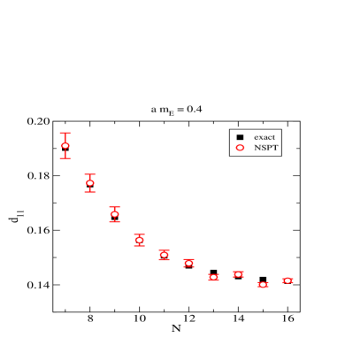
As a check of the first of these extrapolations, we compare the numerical outputs for $d_{11}$ with its known values (eq. (8)) at fixed $am_{\mbox{\tiny\rm{E}}}$ and lattice extent $N$: this is done in Fig. 1.

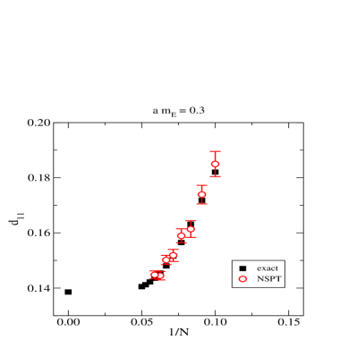
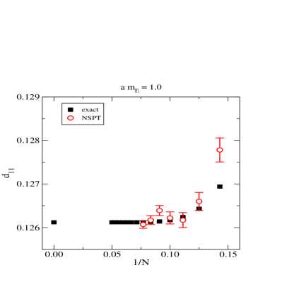
The next task is to extrapolate to infinite volume. As Fig. 1 shows, finite-volume effects become exponentially small at large volumes. However, the volume required for this grows as the mass $am_{\mbox{\tiny\rm{E}}}$ decreases. This is illustrated in Fig. 2 for two masses, one larger than in Fig. 1, and one smaller. For the large mass, a plateau can be reached allowing for a reliable infinite-volume extrapolation, while for the smaller mass, the largest volumes we can afford are not yet large enough to reach a plateau.

In order to deal with this situation, we adopt the following approach. Let us consider a mass like $am_{\mbox{\tiny\rm{E}}}=0.8$: numerical evidence shows that this one has a reasonable plateau at affordable $N$ for all the coefficients $d_{ij}$, but still the behaviour of the data is not too flat (i.e., some volume dependence is detectable). One can then extract an infinite-volume value $d_{ij}(\infty)$ by fitting a constant to data in the range of the plateau, and subtract it from the data in order to obtain the quantities ($L\equiv Na$)

   

Figure 2: Results for the coefficient $d_{11}$ vs. $1/N$ at $am_{\mbox{\tiny\rm{E}}}=0.3$ and $1.0$. Note the very different resolutions of the vertical axes.

$$g_{ij}(m_{\mbox{\tiny\rm{E}}}L)\equiv d_{ij}(m_{\mbox{\tiny\rm{E}}}L)-d_{ij}(\infty)~{}.\vspace{0.2cm}$$ (13)

Subsequently, one can try to obtain a reasonable interpolating fit $f_{ij}(m_{\mbox{\tiny\rm{E}}}L)$ for $g_{ij}(m_{\mbox{\tiny\rm{E}}}L)$, allowing to go also to other values of $m_{\mbox{\tiny\rm{E}}}L$ than those simulated at $am_{\mbox{\tiny\rm{E}}}=0.8$. After this, one can go back to the other masses $m^{\prime}_{\mbox{\tiny\rm{E}}}$, and take a finite-size scaling ansatz of the form

$$d_{ij}(m^{\prime}_{\mbox{\tiny\rm{E}}}L)=d_{ij}(\infty)+A_{ij}(am^{\prime}_{\mbox{\tiny\rm{E}}})\times f_{ij}(m^{\prime}_{\mbox{\tiny\rm{E}}}L)~{},$$ (14)

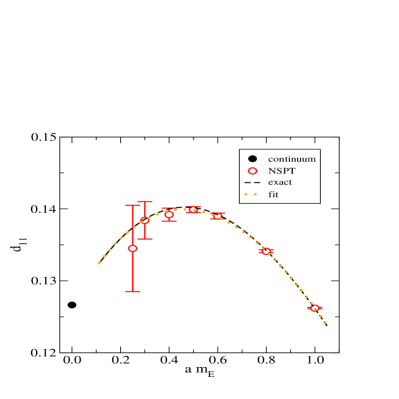
where $d_{ij}(m^{\prime}_{\mbox{\tiny\rm{E}}}L)$ are the direct measurements at the mass $m^{\prime}_{\mbox{\tiny\rm{E}}}$, and $d_{ij}(\infty)$ and $A_{ij}(am^{\prime}_{\mbox{\tiny\rm{E}}})$ are volume-independent fit coefficients. Test results for $d_{11}(\infty)$ obtained this way are shown in Fig. 3.

Figure 3: Comparison between exact values (dashed curve) and numerical infinite-volume extrapolations (open symbols) as a function of $am_{\mbox{\tiny\rm{E}}}$. The continuum value at $am_{\mbox{\tiny\rm{E}}}=0$ has been extracted from ref. [14]. The dotted line shows a fit through the open symbols, constrained to go through the continuum point (which is known for all $d_{ij}$). The agreement between the exact and fitted curves is satisfactory.

6 Conclusions

Preliminary studies of the 2-loop coefficient $d_{11}$, where analytical values are also available, show that our general approach works. The next goal is to finalise the analysis for the most important 3-loop coefficient $d_{20}$ and 4-loop coefficient $d_{30}$ [15]. The quality of our data is good, so we expect to be able to extract these with small errors in the same mass range as in Fig. 3. This should allow to re-analyse the Monte Carlo data of ref. [9] with significantly reduced systematic errors from the continuum extrapolation. Combining with refs. [16, 17, 18], all “soft” contributions to the hot QCD pressure would then be under reasonable control. At the same time, the determination of the 4-loop “hard” contributions remains an open challenge; toy model computations in scalar field theory have suggested, however, that it can be tackled with some effort [19].

References

- [1] P. Arnold and C. Zhai, The three loop free energy for pure gauge QCD, Phys. Rev. D 50 (1994) 7603 [hep-ph/9408276]; The three loop free energy for high temperature QED and QCD with fermions, Phys. Rev. D 51 (1995) 1906 [hep-ph/9410360].
- [2] G. Boyd, J. Engels, F. Karsch, E. Laermann, C. Legeland, M. Lütgemeier and B. Petersson, Thermodynamics of SU(3) lattice gauge theory, Nucl. Phys. B 469 (1996) 419 [hep-lat/9602007].
- [3] G. Endrodi, Z. Fodor, S.D. Katz and K.K. Szabo, The equation of state at high temperatures from lattice QCD, [arXiv:0710.4197].
- [4] P. Ginsparg, First and second order phase transitions in gauge theories at finite temperature, Nucl. Phys. B 170 (1980) 388.
- [5] T. Appelquist and R.D. Pisarski, High-temperature Yang-Mills theories and three-dimensional Quantum Chromodynamics, Phys. Rev. D 23 (1981) 2305.
- [6] K. Kajantie, M. Laine, K. Rummukainen and M. Shaposhnikov, Generic rules for high temperature dimensional reduction and their application to the Standard Model, Nucl. Phys. B 458 (1996) 90 [hep-ph/9508379].
- [7] E. Braaten and A. Nieto, Free energy of QCD at high temperature, Phys. Rev. D 53 (1996) 3421 [hep-ph/9510408].
- [8] J.P. Blaizot, E. Iancu and A. Rebhan, On the apparent convergence of perturbative QCD at high temperature, Phys. Rev. D 68 (2003) 025011 [hep-ph/0303045]; P. Giovannangeli, Two loop renormalization of the magnetic coupling and non-perturbative sector in hot QCD, Nucl. Phys. B 738 (2006) 23 [hep-ph/0506318].
- [9] K. Kajantie, M. Laine, K. Rummukainen and Y. Schröder, How to resum long-distance contributions to the QCD pressure?, Phys. Rev. Lett. 86 (2001) 10 [hep-ph/0007109].
- [10] M. Laine and A. Rajantie, Lattice-continuum relations for 3d SU(N)+Higgs theories, Nucl. Phys. B 513 (1998) 471 [hep-lat/9705003].
- [11] F. Di Renzo, E. Onofri, G. Marchesini and P. Marenzoni, Four loop result in SU(3) lattice gauge theory by a stochastic method: lattice correction to the condensate, Nucl. Phys. B 426 (1994) 675 [hep-lat/9405019].
- [12] H. Panagopoulos, A. Skouroupathis and A. Tsapalis, Free energy and plaquette expectation value for gluons on the lattice, in three dimensions, Phys. Rev. D 73 (2006) 054511 [hep-lat/0601009].
- [13] G. Parisi and Y.S. Wu, Perturbation theory without gauge fixing, Sci. Sin. 24 (1981) 483.
- [14] K. Kajantie, M. Laine, K. Rummukainen and Y. Schröder, Four-loop vacuum energy density of the SU() + adjoint Higgs theory, JHEP 04 (2003) 036 [hep-ph/0304048].
- [15] F. Di Renzo, M. Laine, Y. Schröder and C. Torrero, Four-loop lattice-regularized vacuum energy density of the three-dimensional SU(3) + adjoint Higgs theory, work in progress.
- [16] K. Kajantie, M. Laine, K. Rummukainen and Y. Schröder, The pressure of hot QCD up to , Phys. Rev. D 67 (2003) 105008 [hep-ph/0211321].
- [17] A. Hietanen, K. Kajantie, M. Laine, K. Rummukainen and Y. Schröder, Plaquette expectation value and gluon condensate in three dimensions, JHEP 01 (2005) 013 [hep-lat/0412008]; A. Hietanen and A. Kurkela, Plaquette expectation value and lattice free energy of three-dimensional SU() gauge theory, JHEP 11 (2006) 060 [hep-lat/0609015].
- [18] F. Di Renzo, M. Laine, V. Miccio, Y. Schröder and C. Torrero, The leading non-perturbative coefficient in the weak-coupling expansion of hot QCD pressure, JHEP 07 (2006) 026 [hep-ph/0605042].
- [19] A. Gynther, M. Laine, Y. Schröder, C. Torrero and A. Vuorinen, Four-loop pressure of massless O(N) scalar field theory, JHEP 04 (2007) 094 [hep-ph/0703307].