Modeling homophily and stochastic equivalence in symmetric relational data
Abstract
This article discusses a latent variable model for inference and prediction of symmetric relational data. The model, based on the idea of the eigenvalue decomposition, represents the relationship between two nodes as the weighted inner-product of node-specific vectors of latent characteristics. This “eigenmodel” generalizes other popular latent variable models, such as latent class and distance models: It is shown mathematically that any latent class or distance model has a representation as an eigenmodel, but not vice-versa. The practical implications of this are examined in the context of three real datasets, for which the eigenmodel has as good or better out-of-sample predictive performance than the other two models.
Some key words: Factor analysis, latent class, Markov chain Monte Carlo, social network.
1 Introduction
Let denote data measured on pairs of a set of objects or nodes. The examples considered in this article include friendships among people, associations among words and interactions among proteins. Such measurements are often represented by a sociomatrix , which is a symmetric matrix with an undefined diagonal. One of the goals of relational data analysis is to describe the variation among the entries of , as well as any potential covariation of with observed explanatory variables .
To this end, a variety of statistical models have been developed that describe as some function of node-specific latent variables and and a linear predictor . In such formulations, represent across-node variation in the ’s and represents covariation of the ’s with the ’s. For example, Nowicki and Snijders (2001) present a model in which each node is assumed to belong to an unobserved latent class , and a probability distribution describes the relationships between each pair of classes (see Kemp et al. (2004) and Airoldi et al. (2005) for recent extensions of this approach). Such a model captures stochastic equivalence, a type of pattern often seen in network data in which the nodes can be divided into groups such that members of the same group have similar patterns of relationships.
An alternative approach to representing across-node variation is based on the idea of homophily, in which the relationships between nodes with similar characteristics are stronger than the relationships between nodes having different characteristics. Homophily provides an explanation to data patterns often seen in social networks, such as transitivity (“a friend of a friend is a friend”), balance (“the enemy of my friend is an enemy”) and the existence of cohesive subgroups of nodes. In order to represent such patterns, Hoff et al. (2002) present a model in which the conditional mean of is a function of , where are vectors of unobserved, latent characteristics in a Euclidean space. In the context of binary relational data, such a model predicts the existence of more transitive triples, or “triangles,” than would be seen under a random allocation of edges among pairs of nodes. An important assumption of this model is that two nodes with a strong relationship between them are also similar to each other in terms of how they relate to other nodes: A strong relationship between and suggests is small, but this further implies that , and so nodes and are assumed to have similar relationships to other nodes.

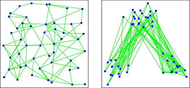
The latent class model of Nowicki and Snijders (2001) and the latent distance model of Hoff et al. (2002) are able to identify, respectively, classes of nodes with similar roles, and the locational properties of the nodes. These two items are perhaps the two primary features of interest in social network and relational data analysis. For example, discussion of these concepts makes up more than half of the 734 pages of main text in Wasserman and Faust (1994). However, a model that can represent one feature may not be able to represent the other: Consider the two graphs in Figure 1. The graph on the left displays a large degree of transitivity, and can be well-represented by the latent distance model with a set of vectors in two-dimensional space, in which the probability of an edge between and is decreasing in . In contrast, representation of the graph by a latent class model would require a large number of classes, none of which would be particularly cohesive or distinguishable from the others. The second panel of Figure 1 displays a network involving three classes of stochastically equivalent nodes, two of which (say and ) have only across-class ties, and one () that has both within- and across-class ties. This graph is well-represented by a latent class model in which edges occur with high probability between pairs having one member in each of and or in and , and among pairs having both members in (in models of stochastic equivalence, nodes within each class are not differentiated). In contrast, representation of this type of graph with a latent distance model would require the dimension of the latent characteristics to be on the order of the class membership sizes.
Many real networks exhibit combinations of structural equivalence and homophily in varying degrees. In these situations, use of either the latent class or distance model would only be representing part of the network structure. The goal of this paper is to show that a simple statistical model based on the eigenvalue decomposition can generalize the latent class and distance models: Just as any symmetric matrix can be approximated with a subset of its largest eigenvalues and corresponding eigenvectors, the variation in a sociomatrix can be represented by modeling as a function of , where are node-specific factors and is a diagonal matrix. In this article, we show mathematically and by example how this eigenmodel can represent both stochastic equivalence and homophily in symmetric relational data, and thus is more general than the other two latent variable models.
The next section motivates the use of latent variables models for relational data, and shows mathematically that the eigenmodel generalizes the latent class and distance models in the sense that it can compactly represent the same network features as these other models but not vice-versa. Section 3 compares the out-of-sample predictive performance of these three models on three different datasets: a social network of 12th graders; a relational dataset on word association counts from the first chapter of Genesis; and a dataset on protein-protein interactions. The first two networks exhibit latent homophily and stochastic equivalence respectively, whereas the third shows both to some degree. In support of the theoretical results of Section 2, the latent distance and class models perform well for the first and second datasets respectively, whereas the eigenmodel performs well for all three. Section 4 summarizes the results and discusses some extensions.
2 Latent variable modeling of relational data
2.1 Justification of latent variable modeling
The use of probabilistic latent variable models for the representation of relational data can be motivated in a natural way: For undirected data without covariate information, symmetry suggests that any probability model we consider should treat the nodes as being exchangeable, so that
for any permutation of the integers and any set of sociomatrices . Results of Hoover (1982) and Aldous (1985, chap. 14) show that if a model satisfies the above exchangeability condition for each integer , then it can be written as a latent variable model of the form
| (1) |
for i.i.d. latent variables , i.i.d. pair-specific effects and some function that is symmetric in its second and third arguments. This result is very general - it says that any statistical model for a sociomatrix in which the nodes are exchangeable can be written as a latent variable model.
Difference choices of lead to different models for . A general probit model for binary network data can be put in the form of (1) as follows:
where and are parameters to be estimated, and is a symmetric function, also potentially involving parameters to be estimated. Covariation between and an array of predictor variables can be represented by adding a linear predictor to . Finally, integrating over we obtain . Since the ’s can be assumed to be independent, the conditional probability of given and can be expressed as
| (2) | |||||
Many relational datasets have ordinal, non-binary measurements (for example, the word association data in Section 3.2). Rather than “thresholding” the data to force it to be binary, we can make use of the full information in the data with an ordered probit version of (2):
where are parameters to be estimated for all but the lowest value in the sample space.
2.2 Effects of nodal variation
The latent variable models described in the Introduction correspond to different choices for the symmetric function :
-
Latent class model:
-
-
-
a symmetric matrix
-
-
Latent distance model:
-
-
Latent eigenmodel:
-
-
-
a diagonal matrix.
-
Interpretations of the latent class and distance models were given in the Introduction. An interpretation of the latent eigenmodel is that each node has a vector of unobserved characteristics , and that similar values of and will contribute positively or negatively to the relationship between and , depending on whether or . In this way, the model can represent both positive or negative homophily in varying degrees, and stochastically equivalent nodes (nodes with the same or similar latent vectors) may or may not have strong relationships with one another.
We now show that the eigenmodel generalizes the latent class and distance models: Let be the set of sociomatrices, and let
In other words, is the set of possible values of under a -dimensional latent class model, and similarly for and .
generalizes :
Let and let be a completion of obtained by setting . There are at most unique rows of and so is of rank at most. Since the set contains all sociomatrices that can be completed as a rank- matrix, we have . Since includes matrices with unique rows, unless in which case the two sets are equal.
weakly generalizes :
Let . Such a (negative) distance matrix will generally be of full rank, in which case it cannot be represented exactly by an for . However, what is critical from a modeling perspective is whether or not the order of the entries of each can be matched by the order of the entries of an . This is because the probit and ordered probit model we are considering include threshold variables which can be adjusted to accommodate monotone transformations of . With this in mind, note that the matrix of squared distances among a set of -dimensional vectors is a monotonic transformation of the distances, is of rank or less (as ) and so is in . Furthermore, letting for each , we have . For large this is approximately , which is an increasing function of the negative distance . For large enough the numerical order of the entries of this is the same as that of .
does not weakly generalize :
Consider generated by , and for . Then for all . For which is such an ordering of the elements of possible? If then such an ordering is possible only if . For such an ordering is possible for . This is because the kissing number in , or the number of non-overlapping spheres of unit radius that can simultaneously touch a central sphere of unit radius, is 6. If we put node 1 at the center of the central sphere, and 6 nodes at the centers of the 6 kissing spheres, then we have for all . We can only have if we remove one of the non-central spheres to allow for more room between those remaining, leaving one central sphere plus five kissing spheres for a total of . Increasing increases the necessary dimension of the Euclidean space, and so for any there are and that have entry orderings that cannot be matched by those of any .
A less general positive semi-definite version of the eigenmodel has been studied by Hoff (2005), in which was taken to be the identity matrix. Such a model can weakly generalize a distance model, but cannot generalize a latent class model, as the eigenvalues of a latent class model could be negative.
3 Model comparison on three different datasets
3.1 Parameter estimation
Bayesian parameter estimation for the three models under consideration can be achieved via Markov chain Monte Carlo (MCMC) algorithms, in which posterior distributions for the unknown quantities are approximated with empirical distributions of samples from a Markov chain. For these algorithms, it is useful to formulate the probit models described in Section 2.1 in terms of an additional latent variable normal, for which if . Using conjugate prior distributions where possible, the MCMC algorithms proceed by generating a new state from a current state as follows:
-
1.
For each , sample from its (constrained normal) full conditional distribution.
-
2.
For each , sample from its (normal) full conditional distribution.
-
3.
Sample from its (multivariate normal) full conditional distribution.
-
4.
Sample and their associated parameters:
-
•
For the latent distance model, propose and accept or reject new values of the ’s with the Metropolis algorithm, and then sample the population variances of the ’s from their (inverse-gamma) full conditional distributions.
-
•
For the latent class model, update each class variable from its (multinomial) conditional distribution given current values of and the variance of the elements of (but marginally over to improve mixing). Then sample the elements of from their (normal) full conditional distributions and the variance of the entries of from its (inverse-gamma) full conditional distribution.
-
•
For the latent vector model, sample each from its (multivariate normal) full conditional distribution, sample the mean of the ’s from their (normal) full conditional distributions, and then sample from its (multivariate normal) full conditional distribution.
-
•
To facilitate comparison across models, we used prior distributions in which the level of prior variability in was similar across the three different models. An R package that implements the MCMC is available at cran.r-project.org/src/contrib/Descriptions/eigenmodel.html.
3.2 Cross validation
To compare the performance of these three different models we evaluated their out-of-sample predictive performance under a range of dimensions () and on three different datasets exhibiting varying combinations of homophily and stochastic equivalence. For each combination of dataset, dimension and model we performed a five-fold cross validation experiment as follows:
-
1.
Randomly divide the data values into 5 sets of roughly equal size, letting be the set to which pair is assigned.
-
2.
For each :
-
(a)
Obtain posterior distributions of the model parameter conditional on , the data on pairs not in set .
-
(b)
For pairs in set , let , the posterior predictive mean of obtained using data not in set .
-
(a)
This procedure generates a sociomatrix , in which each entry represents a predicted value obtained from using a subset of the data that does not include . Thus is a sociomatrix of out-of-sample predictions of the observed data .
| Add health | Genesis | Protein interaction | |||||||
|---|---|---|---|---|---|---|---|---|---|
| dist | class | eigen | dist | class | eigen | dist | class | eigen | |
| 3 | 0.82 | 0.64 | 0.75 | 0.62 | 0.82 | 0.82 | 0.83 | 0.79 | 0.88 |
| 5 | 0.81 | 0.70 | 0.78 | 0.66 | 0.82 | 0.82 | 0.84 | 0.84 | 0.90 |
| 10 | 0.76 | 0.69 | 0.80 | 0.74 | 0.82 | 0.82 | 0.85 | 0.86 | 0.90 |
3.3 Adolescent Health social network

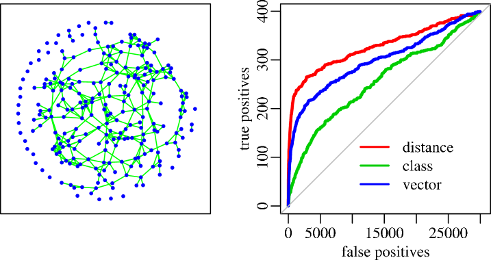
The first dataset records friendship ties among 247 12th-graders, obtained from the National Longitudinal Study of Adolescent Health (www.cpc.unc.edu/projects/addhealth). For these data, or depending on whether or not there is a close friendship tie between student and (as reported by either or ). These data are represented as an undirected graph in the first panel of Figure 2. Like many social networks, these data exhibit a good deal of transitivity. It is therefore not surprising that the best performing models considered (in terms of area under the ROC curve, given in Table 1) are the distance models, with the eigenmodels close behind. In contrast, the latent class models perform poorly, and the results suggest that increasing for this model would not improve its performance.

3.4 Word neighbors in Genesis
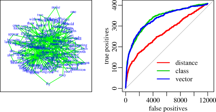
The second dataset we consider is derived from word and punctuation counts in the first chapter of the King James version of Genesis (www.gutenberg.org/dirs/etext05/bib0110.txt). There are 158 unique words and punctuation marks in this chapter, and for our example we take to be the number of times that word and word appear next to each other (a model extension, appropriate for an asymmetric version of this dataset, is discussed in the next section). These data can be viewed as a graph with weighted edges, the unweighted version of which is shown in the first panel of Figure 3. The lack of a clear spatial representation of these data is not unexpected, as text data such as these do not have groups of words with strong within-group connections, nor do they display much homophily: a given noun may appear quite frequently next to two different verbs, but these verbs will not appear next to each other. A better description of these data might be that there are classes of words, and connections occur between words of different classes. The cross validation results support this claim, in that the latent class model performs much better than the distance model on these data, as seen in the second panel of Figure 3 and in Table 1. As discussed in the previous section, the eigenmodel generalizes the latent class model and performs equally well. We note that parameter estimates for these data were obtained using the ordered probit versions of the models (as the data are not binary), but the out-of-sample predictive performance was evaluated based on each model’s ability to predict a non-zero relationship.
3.5 Protein-protein interaction data
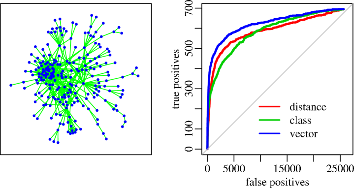
Our last example is the protein-protein interaction data of Butland et al. (2005), in which if proteins and bind and otherwise. We analyze the large connected component of this graph, which includes 230 proteins and is displayed in the first panel of 4. This graph indicates patterns of both stochastic equivalence and homophily: Some nodes could be described as ‘‘hubs’’, connecting to many other nodes which in turn do not connect to each other. Such structure is better represented by a latent class model than a distance model. However, most nodes connecting to hubs generally connect to only one hub, which is a feature that is hard to represent with a small number of latent classes. To represent this structure well, we would need two latent classes per hub, one for the hub itself and one for the nodes connecting to the hub. Furthermore, the core of the network (the nodes with more than two connections) displays a good degree of homophily in the form of transitive triads, a feature which is easiest to represent with a distance model. The eigenmodel is able to capture both of these data features and performs better than the other two models in terms of out-of-sample predictive performance. In fact, the eigenmodel performs better than the other two models for any value of considered.

4 Discussion
Latent distance and latent class models provide concise, easily interpreted descriptions of social networks and relational data. However, neither of these models will provide a complete picture of relational data that exhibit degrees of both homophily and stochastic equivalence. In contrast, we have shown that a latent eigenmodel is able to represent datasets with either or both of these data patterns. This is due to the fact that the eigenmodel provides an unrestricted low-rank approximation to the sociomatrix, and is therefore able to represent a wide array of patterns in the data.
The concept behind the eigenmodel is the familiar eigenvalue decomposition of a symmetric matrix. The analogue for directed networks or rectangular matrix data would be a model based on the singular value decomposition, in which data could be modeled as depending on , where and represent vectors of latent row and column effects respectively. Statistical inference using the singular value decomposition for Gaussian data is straightforward. A model-based version of the approach for binary and other non-Gaussian relational datasets could be implemented using the ordered probit model discussed in this paper.
Acknowledgment
This work was partially funded by NSF grant number 0631531.
References
- Airoldi et al. [2005] Edoardo Airoldi, David Blei, Eric Xing, and Stephen Fienberg. A latent mixed membership model for relational data. In LinkKDD ’05: Proceedings of the 3rd international workshop on Link discovery, pages 82--89, New York, NY, USA, 2005. ACM Press. ISBN 1-59593-215-1. doi: http://doi.acm.org/10.1145/1134271.1134283.
- Aldous [1985] David J. Aldous. Exchangeability and related topics. In École d’été de probabilités de Saint-Flour, XIII---1983, volume 1117 of Lecture Notes in Math., pages 1--198. Springer, Berlin, 1985.
- Butland et al. [2005] G. Butland, J. M. Peregrin-Alvarez, J. Li, W. Yang, X. Yang, V. Canadien, A. Starostine, D. Richards, B. Beattie, N. Krogan, M. Davey, J. Parkinson, J. Greenblatt, and A. Emili. Interaction network containing conserved and essential protein complexes in escherichia coli. Nature, 433:531--537, 2005.
- Hoff [2005] Peter D. Hoff. Bilinear mixed-effects models for dyadic data. J. Amer. Statist. Assoc., 100(469):286--295, 2005. ISSN 0162-1459.
- Hoff et al. [2002] Peter D. Hoff, Adrian E. Raftery, and Mark S. Handcock. Latent space approaches to social network analysis. J. Amer. Statist. Assoc., 97(460):1090--1098, 2002. ISSN 0162-1459.
- Hoover [1982] D. N. Hoover. Row-column exchangeability and a generalized model for probability. In Exchangeability in probability and statistics (Rome, 1981), pages 281--291. North-Holland, Amsterdam, 1982.
- Kemp et al. [2004] Charles Kemp, Thomas L. Griffiths, and Joshua B. Tenenbaum. Discovering latent classes in relational data. AI Memo 2004-019, Massachusetts Institute of Technology, 2004.
- Nowicki and Snijders [2001] Krzysztof Nowicki and Tom A. B. Snijders. Estimation and prediction for stochastic blockstructures. J. Amer. Statist. Assoc., 96(455):1077--1087, 2001. ISSN 0162-1459.
- Wasserman and Faust [1994] Stanley Wasserman and Katherine Faust. Social Network Analysis: Methods and Applications. Cambridge University Press, Cambridge, 1994.