Magnetic properties of bi-phase micro- and nanotubes

Abstract

The magnetic configurations of bi-phase micro- and nanotubes consisting of a ferromagnetic internal tube, an intermediate non-magnetic spacer, and an external magnetic shell are investigated as a function of their geometry. Based on a continuum approach we obtained analytical expressions for the energy which lead us to obtain phase diagrams giving the relative stability of characteristic internal magnetic configurations of the bi-phase tubes.

I Introduction

The fabrication of ultra-highly magnetic recording media has become one of the great challenges in the field of magnetism. It is well known that in conventional recording media, composed of weakly coupled magnetic grains, the areal density is limited by the so-called superparamagnetic effect, Ross which arises as the grain size is reduced below $10$ nm. In such a case, thermal fluctuations in the magnetic moment orientation may lead to loss of information. In order to increase the recording densities, new magnetic elements need to be proposed.

Patterned magnetic media consisting of regular arrays of magnetic layered nanodots Albrecht or nanorings Escrig have been considered as providing the basis for extending magnetic storage densities beyond the superparamagnetic limit. In such systems, a single dot or ring with $n$ magnetic layers, whose volume is much larger than those of the grains in conventional recording media, might store up to 2ⁿ bits, beating thermal fluctuations and increasing the recording density by a factor of 2^n-1.

Recently, magnetic nanotubes can be (chemically) functionalized on the in- and outside, Nielsch ; Nielsch2 ; Wang motivating a new field of research. Nanotubes exhibit a core-free magnetic configuration leading to uniform switching fields, guaranteeing reproducibility Wang ; Escrig2 and have been proposed to be used as bi-directional sensors by Lee et al. Lee Also due to their low density they can float in solutions, making them suitable for biological applications (see [4] and references therein). Numerical simulations Wang ; Landeros and analytical calculations Escrig2 ; Landeros on such tubes have identified two main ideal magnetic configurations: a ferromagnetic state with all the magnetic moments pointing parallel to the axis of the tube ($c=1$) and an in-plane magnetic ordering, namely the flux-closure vortex state ($c=2$). However, in tubes with low aspect ratio $(L/R\leq 10)$, another state with two opposite directed vortices with a domain wall between them can appear. Wang ; Lee Similar nano-objects, bi-phase microwires consisting of two metallic layers, a cylindrical nucleus and an external magnetic microtube, separated by an intermediate nonmagnetic microlayer, have been introduced by Pirota et al. Pirota .

The synthesis of bi-phase microwires and magnetic nanotubes opens the possibility of fabricating bi-phase micro- and nanotubes, where new magnetic phases can appear. Because of the geometry, the internal and external tubes can be close enough to interact via a strong dipolar coupling. This interaction can produce new magnetic states of the cylindrical particle as a whole, Xiao which can be used for particular applications. Besides, we can expect the appearance of new magnetic properties, like the dipolar magnetic bias responsible for the giant magnetoimpedance behavior of amorphous microwires. Sinnecker The possibility of achieving such a, spin-valve-like, hysteresis loop is very attractive because of potential applications to sense magnetic fields in magnetic recording systems.

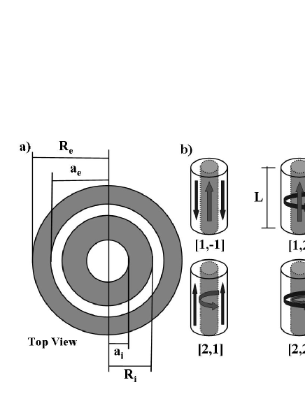
Figure 1: (a) Geometrical parameters and (b) characteristic magnetic configurations of a bi-phase micro- and nanotube.

The purpose of this paper is to investigate the magnetic ordering of bi-phase tubes. Our cylindrical particle, of length $L$, consists of two magnetic tubes separated by a nonmagnetic spacer. The internal (external) tube is characterized by its outer $R_{i}\left(R_{e}\right)$ and inner $a_{i}\left(a_{e}\right)$ radii, as illustrated in figure 1(a). Magnetic configurations of the bi-phase tubes can be identified by two indices $[c_{i},c_{e}]$, where $c_{i},c_{e}=$ 1 or 2 denote the magnetic configurations of the internal and external magnetic tubes, respectively (see figure 1(b)).

II Total energy calculations

We adopt a simplified description of the system, in which the discrete distribution of magnetic moments is replaced by a continuous one characterized by a slowly varying magnetization density $\vec{M}(\vec{r})$. The total energy $E_{tot}^{[c_{i},c_{e}]}$ is generally given by the sum of three terms, the magnetostatic $E_{dip}^{[c_{i},c_{e}]}$, the exchange $E_{ex}^{[c_{i},c_{e}]}$, and the anisotropy contributions. Here we are interested in soft or polycrystalline magnetic materials, in which case the anisotropy contribution is usually disregarded. Nielsch ; Wang

The total magnetization can be written as $\vec{M}(\vec{r})=\vec{M}_{i}\left(\vec{r}\right)+\vec{M}_{e}\left(\vec{r}\right)$, where $\vec{M}_{i}\left(\vec{r}\right)$ and $\vec{M}_{e}\left(\vec{r}\right)$ denote the magnetization of the internal and external tubes, respectively. In this case, the magnetostatic potential $U\left(\vec{r}\right)$ splits up into two components, $U_{i}\left(\vec{r}\right)$ and $U_{e}\left(\vec{r}\right)$, associated with the magnetization of each individual tube. Then, the total dipolar energy can be written as $E_{dip}^{[c_{i},c_{e}]}=E_{d}^{[c_{i}]}+E_{d}^{[c_{e}]}+2E_{d}^{[c_{i},c_{e}]},$ where $E_{d}^{[c_{p},c_{q}]}=\left(\mu_{0}/2\right)\int\vec{M}_{p}\left(\vec{r}\right)\nabla U_{q}\left(\vec{r}\right)\,dv$, with $p,q=i,e$. The diagonal terms, $E_{d}^{[c_{p},c_{p}]}\equiv E_{d}^{[c_{p}]}$, correspond to the dipolar contributions to the self-energy of the individual magnetic tubes, whereas the off-diagonal term, $E_{d}^{[c_{p},c_{q}]}$, corresponds to the dipolar interaction between the two tubes.

The exchange energy $E_{ex}^{[c_{p},c_{q}]}$ also has three contributions, two coming from the direct exchange interaction within the magnetic tubes, and the other one from its indirect interaction mediated by the non-magnetic spacer. We focus on systems in which the thickness of the intermediate tube, $d_{s}=a_{e}-R_{i}$, is large enough to make negligible the indirect exchange interaction between the two magnetic tubes across the non-magnetic one. A good estimate of the range of the indirect exchange interaction can be obtained from results for multilayers.Bloemen In general the interlayer exchange coupling vanishes for spacer thicknesses greater than a few nanometers. Here we focus our attention on those cases in which $d_{s}$ is bigger than $5$ nm, thus, to a good approximation, $E_{ex}^{[c_{p},c_{q}]}$ can be written as $E_{ex}^{[c_{i}]}+E_{ex}^{[c_{e}]}$, with $E_{ex}^{[c_{p}]}=A\int\left[\left(\nabla m_{px}\right)^{2}+\left(\nabla m_{py}\right)^{2}+\left(\nabla m_{pz}\right)^{2}\right]dv,$ Aharoni $\vec{m}_{p}=(m_{px},m_{py},m_{pz})=\vec{M}_{p}/M_{0}$ is the magnetization of tube $p$ normalized to the saturation magnetization $M_{0}$ and $A$ is the stiffness constant of the magnetic material.

The total energy of the multilayered structure can be written in the form $E_{tot}^{[c_{i},c_{e}]}=E_{self}^{[c_{i}]}+E_{self}^{[c_{e}]}+E_{int}^{[c_{i},c_{e}]}$, where $E_{self}^{[c_{p}]}=$ $E_{d}^{[c_{p}]}+E_{ex}^{[c_{p}]}$ is the self-energy of each magnetic tube, and $E_{int}^{[c_{i},c_{e}]}=$ $2E_{d}^{[c_{i},c_{e}]}$ is the (dipolar) interaction energy between them. We now proceed to calculate the energy terms in the expression for $E_{tot}^{[c_{1},c_{2}]}$. Results are given in units of $\mu_{0}M_{0}^{2}l_{ex}^{3}$, i.e, $\tilde{E}=E/\mu_{0}M_{0}^{2}l_{ex}^{3}$, where $l_{ex}=\sqrt{2A/\mu_{0}M_{0}^{2}}$.

In order to perform the integrals in the above expressions, it is necessary to specify the functional form of the magnetization density for each configuration. For $c=1$, $\vec{M}_{p}\left(\vec{r}\right)$ can be approximated by $M_{0}\hat{z}$, where $\hat{z}$ is the unit vector parallel to the axis of the tube. In this case, we find that the reduced self-energies take the form

$$\tilde{E}_{self}^{[1]}(p)=\frac{\pi R_{p}^{2}}{l_{ex}^{3}}\int\limits_{0}^{\infty}\frac{dq}{q^{2}}\left(1-e^{-qL}\right)~{}\left(J_{1}(qR_{p})-\beta_{p}J_{1}(qa_{p})\right)^{2},$$

with $J_{1}(z)$ a Bessel function of first kind. In this case, the exchange contribution to the self-energy vanishes. For $c=2$, $\vec{M}_{p}\left(\vec{r}\right)$ can be approximate by $M_{0}\hat{\phi}$, where $\hat{\phi}$ is the azimuthal unit vector. In such case the dipolar contribution to the self-energy turns out to be equal to zero, and $\tilde{E}_{self}^{[2]}(p)=-\left(\pi L\ln\beta_{p}\right)/l_{ex}$. We have defined $\beta_{p}=a_{p}/R_{p}$.

Regarding the interaction between the magnetic tubes, the only non-zero terms correspond to the case in which both tubes are in the $c=1$ configuration. Due to the condition of perfect flux closure in the vortex configuration, a magnetic tube in such a configuration does not interact with another, independently of the magnetic configuration of the latter. Thus, we end up with just

$$\tilde{E}_{int}^{\left[1,-1\right]}=-\frac{2\pi R_{i}R_{e}}{l_{ex}^{3}}\int\limits_{0}^{\infty}\frac{dq}{q^{2}}\left(1-e^{-qL}\right)\\ \left(J_{1}(qR_{i})-\beta_{i}J_{1}(qa_{i})\right)\left(J_{1}(qR_{e})-\beta_{e}J_{1}(qa_{e})\right)\ .$$

The minus sign in the superscript of $\tilde{E}_{int}^{[1,-1]}$ indicates that the relative orientation of the magnetization of the internal and external tubes is antiparallel. We remark that, due to the dipolar interaction between the tubes, the total energy of the $\left[1,1\right]$ configuration is always larger than the total energy of $\left[1,-1\right]$.

III Results and discussion

We are now in position to investigate the relative stability of the various $[c_{i},c_{e}]$ configurations. We consider nickel ($l_{ex}=8.225$ nm) and cobalt ($l_{ex}=2.849$ nm) magnetic bi-phase tubes. However, to properly describe this geometry we need to deal with five different geometrical parameters. In order to simplify the illustration of our results, we present phase diagrams in terms of $d_{i}/d_{e}$, where $d_{i}=R_{i}-a_{i}$ is the thickness of the internal magnetic tube and $d_{e}=R_{e}-a_{e}$ represents the thickness of the external magnetic shell, as illustrated in figure 2.

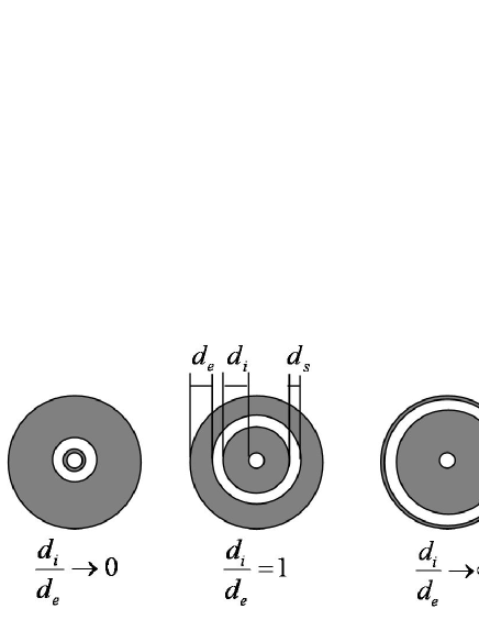
Figure 2: Geometrical parameters and limits of a bi-phase micro- and nanotube.

We start by investigating systems with fixed $a_{i}=10$ nm and $d_{s}=50$ nm. Figure 3 illustrates the phase diagrams, giving the regions within which one of the $[c_{i},c_{e}]$-configurations is of lowest energy for different nanotube lengths. The diagrams show the existence of only three phases, corresponding to the configurations $[1,-1]$, $[1,2]$, and $[2,2]$. The absence of the $\left[2,1\right]$ phase can be understood from the work by Escrig et al. Escrig By inspecting the phase diagram for magnetic tubes presented in that work we can see that, for fixed length, it is easier to find a vortex state for bigger external radius. Then it will be much difficult to find a bi-phase tube with the inner tube in the vortex phase and the external tube, which has a bigger radius than the internal one, in the ferromagnetic phase. The $\left[2,1\right]$ phase is even less probable in this interacting regime, because the dipolar interaction between the tubes will favor the antiferromagnetic-like coupling. By inspecting the energy equation we observe that the $[2,1]$ phase appears only in the limit $d_{i}/d_{e}\rightarrow\infty$. Besides, we observe that a shorter bi-phase tube favors the appearance of vortex configurations. It is worth mentioning that in our model the $[2,-2]$ configuration, corresponding to a vortex and an anti-vortex, and the $[2,2]$ one have the same energy, since in both cases the magnetic nanotubes do not interact. In what follows we shall refer to both as $[2,2]$-configurations. By comparing our results for Ni and Co we observe differences in the behavior of the triple point as a function of $L$. By looking to phase diagrams for isolated tubes, Escrig we observe that a vortex phase appears at smaller external radii of a Co tube than in a Ni one because $l_{ex}(Co)\approx$ $3l_{ex}(Ni)$. This effect is also present in bi-phase tubes, where the triple point occurs for smaller $R_{e}$ in Co. Because $l_{ex}$ is bigger in Ni than in Co, by varying the geometry of the system, the triple point will experience stronger effects in Co than in Ni.

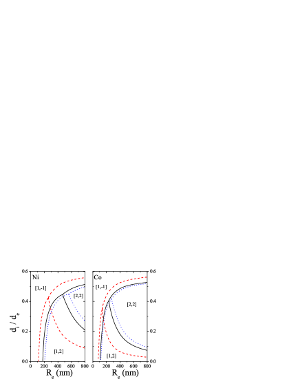
Figure 3: (color online) Variable tube length. Phase diagrams for bi-phase nanotubes with $a_{i}=10$ nm, $d_{s}=50$ nm and $L=1$ $\mu$m (dashed lines), $6$ $\mu$m (solid lines), and $10$  $\mu$m (dotted lines).

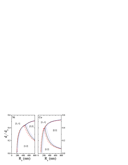
Figure 4: (color online) Variable thickness of the spacer layer. Phase diagrams for bi-phase nanotubes with $a_{i}=10$ nm, $L=6$ $\mu$m and $d_{s}=5$ nm (dashed lines), $50$ nm (solid lines), and $100$  nm (dotted lines).

The dependence of the whole diagram on $d_{s}$ is illustrated in figure 4. In a first inspection of the figures it seems that the main role in this case is played by the material specified in our calculations by $l_{ex}$. However it is important to recall that the ordinate is given by a composed parameter, which makes it complex to determine from the figure the magnetic behavior of the system. Because the interaction between the tubes contributes to stabilize the $[1,-1]$ phase, the decay of the dipolar interaction between the tubes as a function of $d_{s}$ increases the energy of the $[1-1]$ phase, leading to the appearance of the other phases. We illustrate this point with an example. Let us consider a bi-phase Ni tube defined by $a_{i}=10$ nm, $d_{i}=30$ nm, $d_{e}=150$ nm and $L=6$ $\mu$m. In this case $d_{i}/d_{e}=0.2$. If the cylindrical particle is defined by $d_{s}=5$ nm, $R_{e}=195$ nm, and from figure 4 we observe that the nano-object will exhibit a $[1,-1]$ phase. But if for the same geometry we chose $d_{s}=100$, then $R_{e}=290$ and the cylindrical particle will be in the $[1,2]$ phase.

We now turn our attention to the case in which $a_{i}$ is the variable (see figure 5). Here, a strong shift of the transition lines is evidenced as varying the internal radius of the nano-object. In particular, for geometries defined by parameters inside the dark region, the system can exhibit any of three ideal phases, depending on the value of $a_{i}$. Then a clear determination of $a_{i}$ is fundamental when a particular magnetic phase is searched for. In these figures, a clear predominance of the $[1,-1]$ phase appears while increasing $a_{i}$. By increasing $a_{i}$ with fixed $R_{e}$, $d_{s}$ and $d_{i}/d_{e}$, $R_{i}$ and $a_{e}$ necessarily increase. In this way, both tubes have less cross-section area, and then the system prefers the ferromagnetic phase $[1,-1]$.

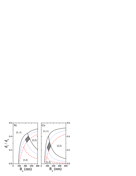
Figure 5: (color online) Variable internal radius $a_{i}$. Phase diagrams for bi-phase nanotubes with $d_{s}=50$ nm, $L=6$ $\mu$m and $a_{i}=$ $10$ nm (solid lines), $30$  nm (dotted lines), and $60$ nm (dashed lines). Inside the dark region, the system can exhibit any of three ideal phases, depending on the value of $a_{i}$.

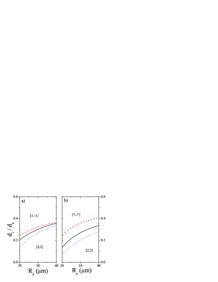
Figure 6: (color online) Phase diagrams for bi-phase microtubes with a) $a_{i}=5$ $\mu$m, $L=1$ cm and $d_{s}=$ $1$ $\mu$m (dashed lines), $5$  $\mu$m (solid lines), and $10$ $\mu$m (dotted lines) and b) $d_{s}=$ $5$ $\mu$m, $L=1$ cm and $a_{i}=$ $3$ $\mu$m (dashed lines), $5$  $\mu$m (solid lines), and $7$ $\mu$m (dotted lines).

We also look to the phase diagrams of bi-phase microtubes. In this case, for the range of diameters and lengths considered, the transition lines are almost independent of the magnetic material. Our results are summarized in figure 6, describing the phases for any magnetic material. Figure 6(a) illustrates the dependence of the phase diagram on $d_{s}$, and figure 6(b) shows the behavior of the whole diagram with $a_{i}$. The diagrams present only two regions, corresponding to the phases $[1,-1]$ and $[2,2]$. The $[1,2]$ phase is suppressed for diameters in the range of the micrometers, as expected from previous figures. Pirota et al. Pirota and Vázquez et al. Vazquez have investigated the magnetic behavior of different multilayer microwires. Hysteresis loops clearly exhibit two Barkhausen jumps, each related to the reversal of one of the tubes. For small values of $d_{i}/d_{e}$, they observe that these Barkhausen jumps are smooth, showing the existence of non-homogeneous states during the reversal of each tube. This qualitative observation is in agreement with our phase diagrams, which show that the $[2,2]$ configurations, which exhibit non-homogeneous reversion, appear preferably for small $d_{i}/d_{e}$. By comparing our results for nano- and microtubes we observe that the $[2,2]$ phase appears preferably in cylindrical particles with large diameters.

In our calculations we considered soft or polycrystalline materials and then anisotropy was disregarded. However, in crystalline materials anisotropy plays a fundamental role, as shown by Escrig et al. Escrig3 In fact, the existence of a strong uniaxial anisotropy, as in Co, favors the $[1,-1]$ phase, decreasing the other two phases, specially the $[2,2]$ one. Nickel has a weak cubic anisotropy with $K<0$, which will enhance the $[2,2]$ phase.

IV Conclusions

In conclusion, we have studied the relative stability of ideal configurations of magnetic bi-phase micro- and nanotubes composed by an internal magnetic tube, an intermediate non-magnetic spacer and an external magnetic shell. In such systems we investigated the size range of the geometric parameters for which different configurations are of lowest energy. Results are summarized in phase diagrams which clearly indicate that the magnetic behavior of such structures can be tailored to meet specific requirements provided a judicious choice of such parameters is made. This includes not just the control over the number of magnetic configurations the system might exhibits, but also the possibility of suppressing specific phases. The lines separating the magnetic phases and, in particular, the triple point, are very sensitive to the geometry of the bi-phase tube. Results in nanotubes strongly depend on the material, defined by its exchange length. However, in microtubes the [1,2] phase is suppressed and the phase diagrams are almost independent of the material. For magnetic bi-phase tubes with diameter of less than 100 nm, the $[1,-1]$ configuration is always present. Besides, we can conclude that for multilayer tubes where total $M_{i}\geq M_{e}$ we always find the antiferromagnetic alignment. The phase diagrams presented can provide guidelines for the production of nanostructures with technological purpose such as the fabrication of sensor devices.

- (1) C. A. Ross, Annual Review of Materials Science 31, 203 (2001).
- (2) M. Albrecht, G. Hu, A. Moser, O. Hellwig, and B. D. Terris, J. Appl. Phys. 97, 103910 (2005).
- (3) J. Escrig, P. Landeros, D. Altbir, M. Bahiana, and J. d’Albuquerque e Castro, Appl. Phys. Lett. 89, 132501 (2006).
- (4) K. Nielsch, F. J. Castano, C. A. Ross, and R. Krishnan, J. Appl. Phys. 98, 034318 (2005).
- (5) Kornelius Nielsch, Fernando J. Castano, Sven Matthias, Woo Lee, and Caroline A. Ross, Adv. Eng. Mat. 7, 217-221 (2005).
- (6) Z. K. Wang et al, Phys. Rev. Lett. 94, 137208 (2005).
- (7) J. Escrig, P. Landeros, D. Altbir, E. E. Vogel, and P. Vargas, J. Magn. Magn. Mater. 308, 233-237 (2007).
- (8) J. Lee, D. Suess, T. Schrefl, Oh K. Hwan, and J. Fidler, J. Magn. Magn. Mater. 310, 2445-2447 (2007).
- (9) P. Landeros, S. Allende, J. Escrig, E. Salcedo, D. Altbir, and E. E. Vogel, Appl. Phys. Lett. 90, 102501 (2007).
- (10) K. Pirota, M. Hernandez-Velez, D. Navas, A. Zhukov, and M. Vázquez, Adv. Funct. Mater. 14, 266-268 (2004).
- (11) Q. Xiao, R. V. Krotkov, and M. T. Tuominen, J. Appl. Phys. 99, 08G305 (2006).
- (12) J. P. Sinnecker, A. de Araujo, R. Piccin, M. Knobel, and M. Vázquez, J. Magn. Magn. Mater. 295, 121-125 (2005).
- (13) P. J. Bloemen, M. T. Johnson, M. T. H. van de Vorst, R. Coehoorn, J. J. de Vries, R. Jungblut, J. van de Stegge, A. Reinders, and W. J. M. de Jong, Phys. Rev. Lett. 72, 764 (1994).
- (14) A. Aharoni, Introduction to the Theory of Ferromagnetism(Oxford: Clarendon Press, 1996) p 135.
- (15) M. Vázquez, K. Pirota, J. Torrejón, G. Badini, and A. Torcunov, J. Magn. Magn. Mater. 304, 197-202 (2006).
- (16) J. Escrig, P. Landeros, D. Altbir, and E. E. Vogel, J. Magn. Magn. Mater. 310, 2448-2450 (2007).