Approximating Perpetuities

Abstract

We propose and analyze an algorithm to approximate distribution functions and densities of perpetuities. Our algorithm refines an earlier approach based on iterating discretized versions of the fixed point equation that defines the perpetuity. We significantly reduce the complexity of the earlier algorithm. Also one particular perpetuity arising in the analysis of the selection algorithm Quickselect is studied in more detail. Our approach works well for distribution functions. For densities we have weaker error bounds although computer experiments indicate that densities can also be approximated well.

Keywords: perpetuity, theory of distributions, approximation of probability densities, perfect simulation

1 Introduction

A perpetuity is a random variable $X$ in $\mathbb{R}$ that satisfies the stochastic fixed-point equation

$$X\stackrel{{\scriptstyle d}}{{=}}AX+b,$$ (1)

where the symbol $\stackrel{{\scriptstyle d}}{{=}}$ denotes that left and right hand side in (1) are identically distributed and where $(A,b)$ is a vector of random variables being independent of $X$, whereas dependence between $A$ and $b$ is allowed.

Perpetuities arise in various different contexts: In discrete mathematics, perpetuities come up as the limit distributions of certain count statistics of decomposable combinatorial structures such as random permutations or random integers. In these areas, perpetuities often arise via relationships to the GEM and Poisson-Dirichlet distributions; see Arratia, Barbour, and Tavaré (2003) for perpetuities, GEM and Poisson-Dirichlet distribution in the context of combinatorial structures; see Donnelly and Grimmett (1993) for occurrences in probabilistic number theory. In the probabilistic analysis of algorithms, perpetuities arise as limit distributions of certain cost measures of recursive algorithms such as the selection algorithm Quickselect, see e.g. Hwang and Tsai (2002) or Mahmoud, Modarres, and Smythe (1995). In insurance and financial mathematics, a perpetuity represents the value of a commitment to make regular payments, where $b$ represents the payment and $A$ a discount factor both being subject to random fluctuation; see, e.g. Goldie and Maller (2000) or Embrechts, Klüppelberg, and Mikosch (1997, Section 8.4).

As perpetuities are given implicitly by their fixed-point characterization (1), properties of their distributions are not directly amenable. Nevertheless, various questions about perpetuities have already been settled. Necessary and sufficient conditions on $(A,b)$ for the fixed-point equation (1) to uniquely determine a probability distribution are discussed in Vervaat (1979) and Goldie and Maller (2000). The types of distributions possible for perpetuities have been identified in Alsmeyer, Iksanov, and Rösler (2007). Tail behavior of perpetuities has been studied for certain cases in Goldie and Grübel (1996).

In the present article, we are interested in the central region of the distributions. The aim is to algorithmically approximate perpetuities, in particular their distribution functions and their Lebesgue densities (if they exist).

For this, we apply and refine a method proposed in Devroye and Neininger (2002) that was originally designed for random variables $X$ satisfying distributional fixed-point equations of the form

$$X\stackrel{{\scriptstyle d}}{{=}}\sum_{r=1}^{K}A_{r}X^{(r)}+b,$$ (2)

where $X^{(1)},\ldots,X^{(K)},(A_{1},\ldots,A_{K},b)$ are independent with $X^{(r)}$ being identically distributed as $X$ for $r=1,\ldots,K$ and random coefficients $A_{1},\ldots,A_{K}$, $b$, and $K\geq 2$.

The case of perpetuities, i.e., $K=1$, structurally differs from the cases $K\geq 2$: The presence of more than one independent copy of $X$ on the right hand side in (2) often has a smoothing effect so that under mild additional assumptions on $(A_{1},\ldots,A_{K},b)$ the existence of smooth Lebesgue densities of $X$ follows, see Fill and Janson (2000) and Devroye and Neininger (2002). On the other hand, the case $K=1$ often leads to distributions ${\cal L}(X)$ that have no smooth Lebesgue density; an example is discussed in Section 5.

Our basic approach to approximate perpetuities is as follows: A random variable $X$ satisfies the distributional identity (1) if and only if its distribution is a fixed-point of the map $T$ on the space $\mathcal{M}$ of probability distributions, given by

$$T:\mathcal{M}\rightarrow\mathcal{M},\ \mu\mapsto\mathcal{L}(AY+b),$$ (3)

where $Y$ is independent of $(A,b)$, and $\mathcal{L}(Y)=\mu$. Under the conditions $\|A\|_{p}<1$ and $\|b\|_{p}<\infty$ for some $p\geq 1$, which we assume throughout the paper, this map is a contraction on certain complete metric subspaces of $\mathcal{M}$. Hence, $\mathcal{L}(X)$ can be obtained as limit of iterations of $T$, starting with some distribution $\mu_{0}$.

However, it is not generally possible to algorithmically compute the iterations of $T$ exactly. We therefore use discrete approximations $(A^{(n)},b^{(n)})$ of $(A,b)$, which become more accurate for increasing $n$, to approximate $T$ by a mapping $\widetilde{T}^{(n)}$, defined by

$$\widetilde{T}^{(n)}:\mathcal{M}\rightarrow\mathcal{M},\ \mu\mapsto\mathcal{L}\!\left(A^{(n)}Y+b^{(n)}\right),$$

where again $Y$ is independent of $(A^{(n)},b^{(n)})$ and $\mathcal{L}(Y)=\mu$.

To allow for an efficient computation of the approximation, we impose a further discretisation step $\left\langle\cdot\right\rangle_{\!n}$, introduced in Section 2, defining

$$T^{(n)}:\mathcal{M}\rightarrow\mathcal{M},\ \mu\mapsto\mathcal{L}\!\left(\left\langle A^{(n)}Y+b^{(n)}\right\rangle_{\!n}\right),$$

where $Y$ is independent of $(A^{(n)},b^{(n)})$ and $\mathcal{L}(Y)=\mu$.

In Section 2, we give conditions for $T^{(n)}\circ T^{(n-1)}\circ\dots\circ T^{(1)}(\mu_{0})$ to converge to the perpetuity given as the solution of (1). To this aim, we derive a rate of convergence in the minimal $L_{p}$ metric $\ell_{p}$, defined on the space $\mathcal{M}_{p}$ of probability measures on $\mathbb{R}$ with finite absolute $p$th moment by

$$\ell_{p}(\nu,\mu)\mathop{:}\!\!=\inf\left\{\left\lVert V-W\bigr{.}\right\rVert_{p}:\ \mathcal{L}(V)=\nu,\mathcal{L}(W)=\mu\right\},\quad\text{ for }\nu,\mu\in\mathcal{M}_{p},$$ (4)

where $\left\lVert\cdot\right\rVert_{p}$ denotes the $L_{p}$-norm of random variables. To get an explicit error bound for the distribution function, we then convert this into a rate of convergence in the Kolmogorov metric $\varrho$, defined by

$$\varrho(\nu,\mu)\mathop{:}\!\!=\sup_{x\in\mathbb{R}}\left\lvert F_{\nu}(x)-F_{\mu}(x)\big{.}\right\rvert,$$

where $F_{\nu},F_{\mu}$ denote the distribution functions of $\nu,\mu\in\mathcal{M}_{p}$. This implies explicit rates of convergence for distribution function and density, depending on the corresponding moduli of continuity of the fixed-point.

For these moduli of continuity we find global bounds for perpetuities with $b\equiv 1$ in Section 4. For cases with random $b$, we have to derive these moduli of continuity individually. One example, connected to the selection algorithm Quickselect, is worked out in detail in Section 5.

We analyze the complexity of our approach in Section 3. As a measure for the complexity of the approximations for distribution function and density, we use the number of steps needed to obtain an approximation that has distance, in supremum norm, of at most $1/n$ to the true function. Although we generally follow the approach in Devroye and Neininger (2002), we can improve the complexity significantly by using different discretisations. For the approximation of the distribution function to an accuracy of $1/n$ in a typical case, we obtain a complexity of $O(n^{1+\varepsilon})$ for any $\varepsilon>0$. In comparison, the algorithm described in Devroye and Neininger (2002), which originally was designed for fixed-point equations of type (2) with $K\geq 2$, would lead to a complexity of $O(n^{4+\varepsilon})$, if applied to our cases. For the approximation of the density to an accuracy of $1/n$, we obtain a complexity of $O(n^{1+1/\alpha+\varepsilon})$ for any $\varepsilon>0$ in the case of $\alpha$-Hölder continuous densities, cf. Corollary 3.2.

An extended abstract of this article appeared in Knape and Neininger (2007+).

2 Discrete approximation and convergence

Recall that our basic assumption in equation (1) is that $\left\lVert A\right\rVert_{p}<1$ and $\left\lVert b\right\rVert_{p}<\infty$ for some $p\geq 1$. To obtain an algorithmically computable approximation of the solution of the fixed-point equation (1), we use an approximation of the sequence defined as follows: We replace $(A,b)$ by a sequence of independent discrete approximations $(A^{(n)},b^{(n)})$, converging to $(A,b)$ in $p$th mean for $n\rightarrow\infty$. To reduce the complexity, we introduce a further discretisation step $\left\langle\cdot\right\rangle_{\!n}$, which reduces the number of values attained by $X_{n}$:

$$X_{0}\mathop{:}\!\!=\bigl{\langle}\mathbb{E}X\bigr{\rangle}_{0},\quad\widetilde{X}_{n}\mathop{:}\!\!=A^{(n)}X_{n-1}+b^{(n)},\quad X_{n}\mathop{:}\!\!=\bigl{\langle}\widetilde{X}_{n}\bigr{\rangle}_{\!n},\quad n\geq 1.$$ (5)

We assume that the discretisations $A^{(n)}$, $b^{(n)}$ and $\left\langle\cdot\right\rangle_{\!n}$ satisfy

$$\left\lVert A^{(n)}-A\right\rVert_{p}\leq R_{A}(n),\quad\left\lVert b^{(n)}-b\right\rVert_{p}\leq R_{b}(n),\quad\left\lVert\bigl{\langle}\widetilde{X}_{n}\bigr{\rangle}_{\!n}-\widetilde{X}_{n}\right\rVert_{p}\leq R_{X}(n),$$ (6)

for some error functions $R_{A}$, $R_{b}$ and $R_{X}$, which we specify later.

Furthermore, we assume that there exists some $\mbox{$\xi\hskip 0.86108pt$}_{\!p}<1$, such that for all $n\geq 1$,

$$\left\lVert A^{(n)}\right\rVert_{p}\!\leq\mbox{$\xi\hskip 0.86108pt$}_{\!p},$$ (7)

which in applications is easy to obtain, since $\|A\|_{p}<1$.

By arguments similar to those used in Fill and Janson (2002) and Devroye and Neininger (2002) we obtain the following convergence rates for the approximations $X_{n}$ to converge to the corresponding characteristics of the fixed-point $X$. We use the shorthand notation $\ell_{p}(X,Y)\mathop{:}\!\!=\ell_{p}(\mathcal{L}(X),\mathcal{L}(Y))$.

Lemma 2.1.

Let $\left(X_{n}\right)_{n\in\mathbb{N}_{0}}$ be defined by (5) and $\mbox{$\xi\hskip 0.86108pt$}_{\!p}$ as in (7). Then

$$\ell_{p}(X_{n},X)\leq\mbox{$\xi\hskip 0.86108pt$}_{\!p}^{n}\,\left\lVert X-X_{0}\right\rVert_{p}+\sum_{i=0}^{n-1}\mbox{$\xi\hskip 0.86108pt$}_{\!p}^{i}\,R(n-i),$$ (8)

where $R(n)\mathop{:}\!\!=R_{X}(n)+R_{A}(n)\left\lVert X\right\rVert_{p}+R_{b}(n)$ for the error functions in (6).

Proof.

We have

$$\ell_{p}(X_{n},X) \leq\ell_{p}(X_{n},\widetilde{X}_{n})+\ell_{p}(\widetilde{X}_{n},X)$$

$$\leq\left\lVert\bigl{\langle}\widetilde{X}_{n}\bigr{\rangle}_{\!n}-\widetilde{X}_{n}\right\rVert_{p}+\ell_{p}(\widetilde{X}_{n},X).$$ (9)

The first summand is bounded by (6) and for the second summand we have

$$\ell_{p}(\widetilde{X}_{n},X) \leq\left\lVert\widetilde{X}_{n}-X\right\rVert_{p}=\left\lVert A^{(n)}X_{n-1}+b^{(n)}-AX-b\right\rVert_{p}$$

$$\leq\left\lVert A^{(n)}X_{n-1}-AX\right\rVert_{p}+\left\lVert b^{(n)}-b\right\rVert_{p}$$

$$=\left\lVert A^{(n)}(X_{n-1}-X)-(A-A^{(n)})X\right\rVert_{p}+\left\lVert b^{(n)}-b\right\rVert_{p}$$

$$\leq\left\lVert A^{(n)}\right\rVert_{p}\left\lVert X_{n-1}-X\right\rVert_{p}+\left\lVert A-A^{(n)}\right\rVert_{p}\left\lVert X\right\rVert_{p}+\left\lVert b^{(n)}-b\right\rVert_{p},$$

where in the last step we use that $A^{(n)}$ and $(X_{n-1}-X)$ as well as $(A-A^{(n)})$ and $X$ are independent by assumption.

Now we use that the infimum in the definition of $\ell_{p}$ in (4) is attained and assume additionally, that $X_{n-1}$ and $X$ are chosen with $\left\lVert X_{n-1}-X\right\rVert_{p}=\ell_{p}(X_{n-1},X)$. Combining this with (2.1) and using the bounds given in (6) and (7), we obtain

$$\ell_{p}(X_{n},X)\leq R_{X}(n)+\mbox{$\xi\hskip 0.86108pt$}_{\!p}\;\ell_{p}(X_{n-1},X)+R_{A}(n)\left\lVert X\right\rVert_{p}+R_{b}(n),$$

and the claim then follows by induction. ∎

To make these estimates explicit we have to specify bounds for $R_{A}(n)$, $R_{b}(n)$, and $R_{X}(n)$. We do so in two different ways, one representing a polynomial discretisation of the corresponding random variables and one representing an exponential discretisation. Better asymptotic results are obtained by the latter one.

Corollary 2.2.

Let $X_{n},n\in\mathbb{N}_{0}$ be defined by (5) and $\mbox{$\xi\hskip 0.86108pt$}_{\!p}$ as in (7), and assume

$$R_{A}(n)\leq C_{A}\,\dfrac{1}{n^{r}},\qquad R_{b}(n)\leq C_{b}\,\dfrac{1}{n^{r}},\qquad R_{X}(n)\leq C_{X}\,\dfrac{1}{n^{r}},$$

for some $r\geq 1$. Then, we have

$$\ell_{p}(X_{n},X)\leq C_{r}\,\frac{1}{n^{r}},$$

where

$$C_{r}:=\frac{r^{r}\,\left\lVert X-X_{0}\right\rVert_{p}}{\Bigl{(}e\,\log\!\left(1/\mbox{$\xi\hskip 0.86108pt$}_{\!p}\right)\Bigr{)}^{r}}+\frac{r!\left(C_{X}+C_{b}+C_{A}\,\left\lVert X\right\rVert_{p}\right)}{\left(1-\mbox{$\xi\hskip 0.86108pt$}_{\!p}\right)^{r+1}}.$$ (10)

Proof.

Using Lemma 2.1 we get

$$\ell_{p}(X_{n},X)\leq\mbox{$\xi\hskip 0.86108pt$}_{\!p}^{n}\left\lVert X-X_{0}\right\rVert_{p}+(C_{X}+C_{A}\left\lVert X\right\rVert_{p}+C_{b})\sum_{i=0}^{n-1}\frac{\mbox{$\xi\hskip 0.86108pt$}_{\!p}^{i}}{\left(n-i\right)^{r}}.$$ (11)

For the first summand, we use that the function $x\mapsto x^{r}\mbox{$\xi\hskip 0.86108pt$}_{\!p}^{x}$ has its maximum at $x=r/\log(1/\mbox{$\xi\hskip 0.86108pt$}_{\!p})$.

To see that the second summand is of order $n^{-r}$, note that $1/(n-i)\leq(i+1)/n$ for all $n\geq 1$ and $0\leq i\leq n-1$. This implies that for $\mbox{$\xi\hskip 0.86108pt$}_{\!p}<1$,

$$\sum_{i=0}^{n-1}\frac{\mbox{$\xi\hskip 0.86108pt$}_{\!p}^{i}}{\left(n-i\right)^{r}} \leq\frac{1}{n^{r}}\sum_{i=0}^{n-1}\left(i+1\right)^{r}\mbox{$\xi\hskip 0.86108pt$}_{\!p}^{i}$$

$$\leq\frac{1}{n^{r}}\sum_{i=0}^{\infty}(i+r)(i+r-1)\dotsm(i+1)\mbox{$\xi\hskip 0.86108pt$}_{\!p}^{i}$$

$$=\frac{r!}{\left(1-\mbox{$\xi\hskip 0.86108pt$}_{\!p}\right)^{r+1}}\,\frac{1}{n^{r}},$$

where the last equality is obtained by differentiating the geometric series $r$ times. ∎

Remark 2.3.

In Corollary 2.2, we are merely interested in the order of magnitude of $\ell_{p}(X_{n},X)$ without a sharp estimate of the constant $C_{r}$. When evaluating the error in an explicit example, we can evaluate (11) directly to obtain sharper estimates.

Corollary 2.4.

Let $X_{n},n\in\mathbb{N}_{0}$ be defined by (5) and $\mbox{$\xi\hskip 0.86108pt$}_{\!p}$ as in (7), and assume

$$R_{A}(n)\leq C_{A}\,\dfrac{1}{\gamma^{n}},\qquad R_{b}(n)\leq C_{b}\,\dfrac{1}{\gamma^{n}},\qquad R_{X}(n)\leq C_{X}\,\dfrac{1}{\gamma^{n}},$$

for some $1<\gamma<1/\mbox{$\xi\hskip 0.86108pt$}_{\!p}$. Then, we have

$$\ell_{p}(X_{n},X)\leq C_{\gamma}\,\frac{1}{\gamma^{n}},$$

where

$$C_{\gamma}:=\left\lVert X-X_{0}\right\rVert_{p}+\frac{\left(C_{X}+C_{b}+C_{A}\,\left\lVert X\right\rVert_{p}\right)}{1-\mbox{$\xi\hskip 0.86108pt$}_{\!p}\gamma}.$$ (12)

Proof.

Using Lemma 2.1 we get

$$\ell_{p}(X_{n},X)\leq\mbox{$\xi\hskip 0.86108pt$}_{\!p}^{n}\left\lVert X-X_{0}\right\rVert_{p}+(C_{X}+C_{A}\left\lVert X\right\rVert_{p}+C_{b})\gamma^{-n}\sum_{i=0}^{n-1}\mbox{$\xi\hskip 0.86108pt$}_{\!p}^{i}\gamma^{i},$$ (13)

and the assumption on $\gamma$ implies that both summands are $O(\gamma^{-n})$ with the constant given in the lemma. ∎

Lemma 2.5.

Let $X_{n}$ and $C_{r}$ be as in Corollary 2.2 and $X$ have a bounded density $f_{X}$. Then, the distance in the Kolmogorov metric can be bounded by

$$\varrho(X_{n},X)\leq\left(C_{r}\left(p+1\right)^{1/p}\left\lVert f_{X}\right\rVert_{\infty}\right)^{p/(p+1)}n^{-rp/(p+1)}.$$ (14)

Similarly, for $X_{n}$ and $C_{\gamma}$ as in Corollary 2.4, we have

$$\varrho(X_{n},X)\leq\left(C_{r}\left(p+1\right)^{1/p}\left\lVert f_{X}\right\rVert_{\infty}\right)^{p/(p+1)}\gamma^{pn/(p+1)}.$$ (15)

Proof.

We use Lemma 5.1 in Fill and Janson (2002), which states, that for $X$ with bounded density $f_{X}$ and any $Y$,

$$\varrho(Y,X)\leq\left(\left(p+1\right)^{1/p}\left\lVert f_{X}\right\rVert_{\infty}\,\ell_{p}(Y,X)\right)^{p/(p+1)}\quad\text{for }p\geq 1.$$

Using Corollaries 2.2 and 2.4 respectively, we get the stated result. ∎

Remark 2.6.

In some cases, we can give a similar bound, although the density of $X$ is not bounded or no explicit bound is known. Instead, it is sufficient to have a bound for the modulus of continuity of the distribution function $F_{X}$ of $X$, cf. Knape (2006).

To approximate the density of the fixed-point, we define

$$f_{n}(x)=\frac{F_{n}(x+\delta_{n})-F_{n}(x-\delta_{n})}{2\delta_{n}},$$ (16)

where $F_{n}$ is the distribution function of $X_{n}$. For this approximation we can give a rate of convergence, depending on the modulus of continuity of the density of the fixed-point, which is defined by

$$\Delta_{f_{X}}(\delta)\mathop{:}\!\!=\!\!\sup_{\begin{subarray}{c}u,v\in\mathbb{R}\\ \left\lvert u-v\right\rvert\leq\delta\end{subarray}}\!\left\lvert f_{X}(u)-f_{X}(v)\bigr{.}\right\rvert,\quad\delta\geq 0.$$

Lemma 2.7.

Let $X$ have a density $f_{X}$ and let $X_{n},n\in\mathbb{N}_{0}$ be defined by (5). Then, for $f_{n}$ defined by (16) and all $\delta_{n}>0$,

$$\left\lVert f_{n}-f_{X}\bigl{.}\right\rVert_{\infty}\leq\frac{1}{\delta_{n}}\;\varrho(X_{n},X)+\Delta_{f_{X}}\!\left(\delta_{n}\right).$$

Proof.

For any $x$, we have

$$\left\lvert f_{n}(x)-f_{X}(x)\bigl{.}\right\rvert \leq\left\lvert\frac{F_{n}(x+\delta_{n})-F_{n}(x-\delta_{n})}{2\delta_{n}}-\frac{F(x+\delta_{n})-F(x-\delta_{n})}{2\delta_{n}}\right\rvert+$$

$$\qquad\qquad+\left\lvert\frac{F(x+\delta_{n})-F(x-\delta_{n})}{2\delta_{n}}-f_{X}(x)\right\rvert$$

$$\leq\frac{1}{\delta_{n}}\;\varrho(X_{n},X)+\frac{1}{2\delta_{n}}\int_{-\delta_{n}}^{\delta_{n}}\!\left\lvert f_{X}(x+y)-f_{X}(x)\big{.}\right\rvert dy$$

$$\leq\frac{1}{\delta_{n}}\varrho(X_{n},X)+\frac{1}{\delta_{n}}\int_{0}^{\delta_{n}}\!\!\!\Delta_{f_{X}}\!(y)\,dy.$$

The assertion follows since $\Delta_{f_{X}}$ is monotonically increasing. ∎

Corollary 2.8.

Let $X$ have a bounded density $f_{X}$, which is Hölder continuous with exponent $\alpha\in(0,1]$. For polynomial discretisation $X_{n}$ and $C_{r}$ as in Corollary 2.2 and $f_{n}$ defined by (16) with

$$\delta_{n}\mathop{:}\!\!=L\,n^{-rp/\left((\alpha+1)(p+1)\right)}$$

with an $L>0$, we have

$$\left\lVert f_{n}-f_{X}\right\rVert_{\infty}\leq\left(\left(C_{r}\left(p+1\right)^{1/p}\left\lVert f_{X}\right\rVert_{\infty}\right)^{p/(p+1)}\!\!\!/L+c\,L^{\alpha}\right)\,n^{-\alpha rp/\left((\alpha+1)(p+1)\right)}.$$

For exponential discretisation $X_{n}$ and $C_{\gamma}$ as in Corollary 2.4 and $f_{n}$ defined by (16) with

$$\delta_{n}\mathop{:}\!\!=L\,\gamma^{-pn/\left((\alpha+1)(p+1)\right)},$$

with an $L>0$, we obtain

$$\left\lVert f_{n}-f_{X}\right\rVert_{\infty}\leq\left(\left(C_{\gamma}\left(p+1\right)^{1/p}\left\lVert f_{X}\right\rVert_{\infty}\right)^{p/(p+1)}\!\!\!/L+c\,L^{\alpha}\right)\,\gamma^{\alpha pn/\left((\alpha+1)(p+1)\right)}.$$

Remark 2.9.

If $X$ is bounded and bounds for the density $f_{X}$ and its modulus of continuity are known explicitly, the last result is strong enough to construct a perfect simulation algorithm based on von Neumann’s rejection method. Corollary 2.8 can be turned into such an algorithm as done in Devroye (2001) for the case of infinitely divisible perpetuities with approximation of densities by Fourier inversion, Devroye, Fill, and Neininger (2000) for the case of the Quicksort limit distribution and Devroye and Neininger (2002) for more general fixed-point equations of type (2).

3 Algorithm and Complexity

In this section, we will give an algorithm for an approximation satisfying the assumptions in the last section for many important cases. We assume that the distributions of $A$ and $b$ are given by Skorohod representations, i.e. by measurable functions $\varphi,\psi:[0,1]\!\rightarrow\!\mathbb{R}$, such that

$$A=\varphi(U)\quad\text{and}\quad b=\psi(U),$$ (17)

$U$ being uniformly distributed on $[0,1]$. Furthermore, we assume that $\left\lVert\varphi\right\rVert_{\infty}\leq 1$ and that both functions are Lipschitz continuous and can be evaluated in constant time. Now we define the discretisation $\left\langle\cdot\right\rangle_{\!n}$ by

$$\left\langle Y\right\rangle_{\!n}:=\left\lfloor s(n)\,Y\right\rfloor\!/s(n),$$ (18)

where $s(n)$ can be either polynomial, i.e. $s(n)=n^{r}$ or exponential, $s(n)=\gamma^{n}$. Defining

$$A^{(n)} \mathop{:}\!\!=\varphi\!\left(\left\langle U\right\rangle_{\!n}\right)\quad\text{and}$$

$$b^{(n)} \mathop{:}\!\!=\psi\!\left(\left\langle U\right\rangle_{\!n}\right),$$

the conditions on $\varphi$ and $\psi$ ensure that Corollary 2.2 and 2.4 can be applied.

We keep the distribution of $X_{n}$ in an array $\mathcal{A}_{n}$, where

$$\mathcal{A}_{n}[k]\mathop{:}\!\!=\mathbb{P}\!\left[X_{n}={k}/{s(n)}\right]$$

for $k\in\mathbb{Z}$. Note however, that as $A$ and $b$ are bounded, $\mathcal{A}_{n}[k]=0$ at least for $\left\lvert k\right\rvert>s(n)Q_{n}$, where $Q_{n}$ can be computed recursively as $Q_{n}=\left\lceil\left\lVert A\right\rVert_{\infty}Q_{n-1}+\left\lVert b\right\rVert_{\infty}\right\rceil$ and $Q_{0}=\left\lceil\left\lVert X_{0}\right\rVert_{\infty}\right\rceil\!=\left\lceil\mathbb{E}X\right\rceil$.

For simplicity we assume that $s(0)=s(1)=1$ and that $s(n)\in\mathbb{N}$ for all $n$. The core of the implementation is the following update procedure:

procedure update($\mathcal{A}_{n-1},\mathcal{A}_{n}$)

     for $i$ $\leftarrow$ $0$ to $s(n)-1$ do

         for $j$ $\leftarrow$ $-\,s(n-1)\,Q_{n-1}$ to $s(n-1)\,Q_{n-1}$ do

              

$$u\quad\leftarrow\quad\frac{i}{s(n)}$$

$$k\quad\leftarrow\quad\left\lfloor s(n)\,\left(\varphi(u)\,\frac{j}{s(n-1)}+\psi(u)\right)\right\rfloor\hskip 10.00002pt$$

$$\mathcal{A}_{n}[k]\leftarrow\hskip 2.15277pt\mathcal{A}_{n}[k]+\frac{1}{s(n)}\,\mathcal{A}_{n-1}[j]$$

         end for

     end for

end procedure

Furthermore, we use a procedure $\textsc{initialize}(\mathcal{A}_{n},n)$, which creates $\mathcal{A}_{n}$ as vector with $2s(n)Q_{n}$ components with $\mathcal{A}_{n}[k]=0$ for $-s(n)Q_{n}\leq k\leq s(n)Q_{n}$.

The whole algorithm then looks like this:

initialize($\mathcal{A}_{0},0$)

$$\mathcal{A}_{0}\!\left[\biggr{.}\left\lfloor\Bigr{.}s(0)\;\mathbb{E}X\right\rfloor\right]\leftarrow 1$$ (19)

for $n$ $\leftarrow$ $1$ to $N$ do

     initialize($\mathcal{A}_{n},n$)

     update($\mathcal{A}_{n-1},\mathcal{A}_{n}$)

end for

return $\mathcal{A}_{N}$

Note, that (19) determines that we start the approximation with $X_{0}$ as defined in (5).

The complete code for polynomial discretisation for the example in Section 5, implemented in C++, can be found in Knape (2006).

To approximate the density as in (16) with $\delta_{N}=d/s(N)$ for some $d\in\mathbb{N}$, we compute a new array $\mathcal{D}_{N}$ by setting

$$\mathcal{D}_{N}[k]=\frac{s(N)}{2d}\sum_{j=k-d+1}^{k+d}\!\!\!\!\mathcal{A}_{N}[j].$$

To measure the complexity of our algorithm, we estimate the number of steps needed to approximate the distribution function and the density up to an accuracy of $1/n$. For the case that $X$ has a bounded density $f_{X}$ which is Hölder continuous, we give asymptotic bounds for polynomial as well as for exponential discretisation. We assume the general condition (17).

Lemma 3.1.

Assume that $X$ has a bounded density $f_{X}$, which is Hölder continuous with exponent $\alpha\in(0,1]$. Using polynomial discretisation with exponent $r$, cf. Corollary 2.2, we can calculate for any $n\in\mathbb{N}$ approximations $\hat{F},\hat{f}$ of the distribution function $F$ and the density $f$ of $X$ with

$$\left\lVert\hat{F}-F\right\rVert_{\infty}\leq\frac{1}{n},\qquad\left\lVert\hat{f}-f\right\rVert_{\infty}\leq\frac{1}{n}$$

in time $T_{F}(n)$ and $T_{f}(n)$ respectively with

$$T_{F}(n)=O\!\left(n^{(2+2/r)(p+1)/p}\right)\quad\text{and}\quad T_{f}(n)=O\!\left(n^{2\left(1+1/\alpha\right)(r+1)(p+1)/(rp)}\right).$$

Using exponential discretisation with parameter $\gamma$ as in Corollary 2.4, approximation to the same accuracy takes time

$$T^{\prime}_{F}(n)=O\!\left(n^{(p+1)/p}\log{n}\right)\quad\text{and}\quad T^{\prime}_{f}(n)=O\!\left(n^{(1+1/\alpha)(p+1)/p}\log{n}\right)$$

for the distribution function and the density of $X$ respectively.

Proof.

In one execution of update($\mathcal{A}_{k-1},\mathcal{A}_{k}$), the outer loop is executed $s(k)$ times. The assumptions on $A$ and $b$ ensure that $Q_{k}=O(k)$, so we have $O(k\,s(k))$ runs of the inner loop and the whole procedure takes time $O\!\left(k\;s(k)^{2}\right)$. Hence, for any $N\in\mathbb{N}$, finding $\mathcal{A}_{N}$ costs time

$$O\!\left(\sum_{k=1}^{N}k\,s(k)^{2}\right)=O\!\left(N^{2}\,s\!\left(N\right)^{2}\right).$$ (20)

For discretisations with $s(n)=n^{r}$ we get a running time of $O(N^{2r+2})$ to find $\mathcal{A}_{N}$, and (14) in Lemma 2.5 ensures that for the corresponding distribution function $F_{N}$ of $X_{N}$,

$$\left\lVert F_{N}-F\right\rVert_{\infty}\leq CN^{-rp/(p+1)}.$$

Setting $N=\left(Cn\right)^{(p+1)/(rp)}$ and $\hat{F}\mathop{:}\!\!=F_{N}$, we get an approximation of the stated accuracy in time

$$T_{F}(n)=O(N^{2r+2})=O(n^{(2+2/r)(p+1)/p}).$$

For the density of $X$ we use Corollary 2.8 and $N^{\prime}=\left(C^{\prime}n\right)^{(\alpha+1)(p+1)/(\alpha rp)}$ to obtain the stated bound.

When using exponential discretisation, $s(n)=\gamma^{n}$, we need time $O(N^{2}\gamma^{N})$ to find $\mathcal{A}_{N}$. Using the corresponding results in Lemma 2.5 and Corollary 2.8 ensures the stated running times. ∎

Corollary 3.2.

Assume (17) and that $X$ has a bounded density $f_{X}$, which is Hölder continuous with exponent $\alpha\in(0,1]$. Then, using exponential discretisation as in Corollary 2.4, approximation to an accuracy of $1/n$ takes time $O(n^{1+\varepsilon})$ for the distribution function and time $O(n^{1+1/\alpha+\varepsilon})$ for the density of $X$ for all $\varepsilon>0$.

Proof.

Note that $\left\lVert\varphi\right\rVert_{\infty}\leq 1$ and $\left\lVert A\right\rVert_{p}<1$ for some $p\geq 1$ implies that $\left\lVert A\right\rVert_{p}<1$ for all $p\geq 1$. Thus, in Lemma 3.1, $p$ can be chosen arbitrarily large. ∎

4 A simple class of perpetuities

In order to make the bounds of Section 2 explicit in applications, we need to bound the absolute value and modulus of continuity of the density of the fixed-point. For a simple class of fixed-point equations, we give universal bounds in this section. For more complicated cases, bounds have to be derived individually, which we work out for one example in Section 5.

For fixed-point equations of the form

$$X\stackrel{{\scriptstyle d}}{{=}}AX+1\qquad\text{with }A\geq 0,$$ (21)

where $A$ and $X$ are independent, we can bound the density and modulus of continuity of $X$ using the corresponding values of $A$.

Lemma 4.1.

Let $X$ satisfy fixed-point equation (21) and $A$ have a density $f_{A}$. Then $X$ has a density $f_{X}$ satisfying

$$f_{X}(u)=\int_{1}^{\infty}\frac{1}{x}\;f_{A}\!\left(\!\frac{u-1}{x}\!\right)f_{X}(x)dx,\quad\text{ for }u\geq 1,$$ (22)

and $f_{X}(u)=0$ otherwise.

Proof.

From the fixed-point equation we can see that $X\geq 1$ almost surely. Now let $\mathbb{P}_{X}$ be the distribution of $X$. Conditioning on $X$, we get for any Borel set $B$:

$$\mathbb{P}\!\left[X\in B\right] =\int_{1}^{\infty}\!\!\mathbb{P}\!\left[Ax+1\in B\right]d\mathbb{P}_{X}(x)$$

$$=\int_{1}^{\infty}\!\!\!\int_{B}f_{xA+1}(u)du\,d\mathbb{P}_{X}(x)$$

$$=\int_{1}^{\infty}\!\!\!\int_{B}\frac{1}{x}\;f_{A}\!\left(\!\frac{u-1}{x}\!\right)du\,d\mathbb{P}_{X}(x)$$

$$=\int_{B}\int_{1}^{\infty}\frac{1}{x}\;f_{A}\!\left(\!\frac{u-1}{x}\!\right)d\mathbb{P}_{X}(x)\;du,$$

where we can use Fubini’s theorem in the last step, because the integrand is product measurable. The claim follows, as this is just the definition of a Lebesgue density. ∎

Corollary 4.2.

Let $A$ have a bounded density $f_{A}$. Then $X$ has a density $f_{X}$ satisfying

$$\left\lVert f_{X}\right\rVert_{\infty}\leq\left\lVert f_{A}\right\rVert_{\infty}.$$

Proof.

Using Lemma 4.1 we get

$$\left\lVert f_{X}\right\rVert_{\infty}\leq\left\lVert f_{A}\right\rVert_{\infty}\,\mathbb{E}\!\left[\frac{1}{X}\right],$$

but $X\geq 1$ implies $\mathbb{E}\!\left[1/X\right]\leq 1$, so the claim follows. ∎

Corollary 4.3.

Let $A$ have a density $f_{A}$, and $\Delta_{f_{A}}$ be its modulus of continuity. Then the modulus of continuity $\Delta_{f_{X}}$ of $f_{X}$ satisfies

$$\Delta_{f_{X}}(\delta)\leq\Delta_{f_{A}}(\delta),\quad\delta>0.$$

Proof.

Using (22), we obtain for any $u,v\in\mathbb{R}$

$$\left\lvert f_{X}(u)-f_{X}(v)\bigr{.}\right\rvert\leq\int_{1}^{\infty}\frac{1}{x}f_{X}(x)\left\lvert f_{A}\left(\!\frac{u-1}{x}\right)-f_{A}\left(\!\frac{v-1}{x}\right)\right\rvert dx.$$ (23)

But $x\geq 1$ and the modulus of continuity $\Delta_{f_{A}}$ is monotonically increasing by definition, so we can bound

$$\left\lvert f_{A}\left(\!\frac{u-1}{x}\right)-f_{A}\left(\!\frac{v-1}{x}\right)\right\rvert\leq\Delta_{f_{A}}\left(\!\frac{\left\lvert u-v\right\rvert}{x}\right)\leq\Delta_{f_{A}}(\left\lvert u-v\right\rvert),$$

and plugging this into inequality (23), we obtain

$$\left\lvert f_{X}(u)-f_{X}(v)\bigr{.}\right\rvert\leq\mathbb{E}\!\left[\frac{1}{X}\right]\,\Delta_{f_{A}}(\left\lvert u-v\right\rvert).$$

Now we use that $\mathbb{E}\!\left[1/X\right]\leq 1$ and take the supremum over all suitable $u,v$. ∎

This result is only useful if the density of $A$ is continuous, but we can extend it to many practical examples, where $f_{A}$ has jumps at points in a set $\mathcal{I}_{A}$. We use the jump function of $f_{A}$, defined by

$$J_{f_{A}}(s)=f_{A}(s)-\lim_{x\uparrow s}f_{A}(x),\quad s>0$$

and a modification of $f_{A}$ where we remove all jumps,

$$\bar{f}_{A}:=f_{A}-\sum_{s\in\mathcal{I}_{A}\setminus\{0\}}J_{f_{A}}(s)\mathbbm{1}_{[s,\infty)}.$$

Since $X\geq 1$, we now denote by $\Delta_{f_{X}}$ the modulus of continuity of the restriction of $f_{X}$ to $(1,\infty)$.

Lemma 4.4.

Let $A$ have a bounded càdlàg density $f_{A}$. Then, for all $\delta>0$,

$$\Delta_{f_{X}}(\delta)\leq\Delta_{\bar{f}_{A}}(\delta)+\left\lVert f_{X}\right\rVert_{\infty}\!\!\sum_{s\in\mathcal{I}_{A}\setminus\{0\}}\!\!\!\frac{\left\lvert J_{f_{A}}(s)\right\rvert\delta}{s}.$$

Proof.

We give the proof for the case that $f_{A}$ has only one jump, say in $s_{0}>0$. The general case then follows similarly. For $1\leq u<v$, we have

$$\left\lvert f_{X}(u)-f_{X}(v)\bigr{.}\right\rvert\leq\int_{1}^{\infty}\frac{1}{x}f_{X}(x)\left\lvert f_{A}\!\!\left(\!\frac{u-1}{x}\!\right)-f_{A}\!\!\left(\!\frac{v-1}{x}\!\right)\right\rvert dx.$$

We define

$$\alpha\mathop{:}\!\!=\frac{u-1}{s_{0}}\vee 1,\quad\beta\mathop{:}\!\!=\frac{v-1}{s_{0}}\vee 1$$

and divide the range of integration into the three intervals $(1,\alpha],[\alpha,\beta],$ and $[\beta,\infty)$. Now, in the first and third interval, differences of values of $f_{A}$ and $\bar{f}_{A}$ coincide. Moreover, for $x\in[\alpha,\beta]$ we have

$$\left\lvert f_{A}\!\left(\!\frac{u-1}{x}\!\!\right)-f_{A}\!\left(\!\frac{v-1}{x}\!\!\right)\right\rvert \leq\left\lvert\bar{f}_{A}\!\!\left(\!\frac{u-1}{x}\!\right)-\bar{f}_{A}\!\!\left(\!\frac{v-1}{x}\!\right)\right\rvert+\left\lvert J_{f_{A}}(s_{0})\bigr{.}\right\rvert.$$

Putting everything together we obtain

$$\left\lvert f_{X}(v)-f_{X}(u)\big{.}\right\rvert\leq$$

$$\leq\int_{1}^{\infty}\!\frac{1}{x}f_{X}(x)\left\lvert\bar{f}_{A}\!\left(\!\frac{u-1}{x}\!\right)-\bar{f}_{A}\!\left(\!\frac{v-1}{x}\!\right)\right\rvert dx+\int_{\alpha}^{\beta}\frac{1}{x}f_{X}(x)\left\lvert J_{f_{A}}(s_{0})\big{.}\right\rvert dx$$

$$\leq\int_{1}^{\infty}\!\frac{1}{x}f_{X}(x)\left\lvert\bar{f}_{A}\!\left(\!\frac{u-1}{x}\!\right)-\bar{f}_{A}\!\left(\!\frac{v-1}{x}\!\right)\right\rvert dx+\left\lVert f_{X}\right\rVert_{\infty}\frac{v-u}{s_{0}}\left\lvert J_{f_{A}}(s_{0})\big{.}\right\rvert.$$

We now bound the latter integral by $\Delta_{\bar{f}_{A}}(v-u)$ as in Corollary 4.3, and the claim follows by taking the supremum over all $v-u\leq\delta$. ∎

5 Example: Number of key exchanges in Quickselect

In this section, we apply our algorithm to the fixed-point equation

$$X\stackrel{{\scriptstyle d}}{{=}}UX+U(1-U),$$ (24)

where $U$ and $X$ are independent and $U$ is uniformly distributed on $[0,1]$. This equation appears in the analysis of the selection algorithm Quickselect. The asymptotic distribution of the number of key exchanges executed by Quickselect when acting on a random equiprobable permutation of length $n$ and selecting an element of rank $k=o(n)$ can be characterized by the above fixed-point equation, see Hwang and Tsai (2002).

We use our algorithm to get a discrete approximation of the fixed point. The plot of a histogram, generated with $80$ iterations of the algorithms using for the discretisation $s(n)=n^{3}$, can be found in Figure 1.

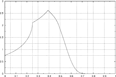
Figure 1: Histogram of approximation for $X\stackrel{{\scriptstyle d}}{{=}}UX+U(1-U)$.

In the following, we specify how the bounds in Section 2 can be made explicit for this example.

Lemma 5.1.

Let $X$ be a solution of (24). Then, we have $0\leq X\leq 1$ almost surely, and the moments are recursively given by $\mathbb{E}\!\left[X^{0}\right]=1$ and

$$\mathbb{E}\!\left[X^{k}\right]=(k+1)!\,(k-1)!\sum_{j=0}^{k-1}\frac{\mathbb{E}\!\left[X^{j}\right]}{j!(2k-j+1)!},\quad k\geq 1,$$

in particular, $\mathbb{E}\!\left[X\right]=1/3$.

Proof.

Both claims follow directly from the fixed-point equation in (24), using that the solution is unique. To compute the moments, note that $\mathbb{E}\!\left[U^{k}(1-U)^{k-j}\right]$ is equal to the Beta function $\mathrm{B}(k+1,k-j+1)$, so we have

$$\mathbb{E}\!\left[X^{k}\right] =\frac{1}{1-\mathbb{E}\!\left[U^{k}\right]}\,\sum_{j=0}^{k-1}\binom{k}{j}\mathbb{E}\!\left[X^{j}\right]\mathrm{B}(k+1,k-j+1)$$

$$=\frac{k+1}{k}\,\sum_{j=0}^{k-1}\frac{k!}{j!(k-j!)}\,\frac{k!(k-j)!}{(2k-j+1)!}\,\mathbb{E}\!\left[X^{j}\right]$$

and the assertion follows. ∎

Lemma 5.2.

Let $X$ be a solution of (24). Then, for all $\kappa\in\mathbb{N}$ and $\varepsilon>0$,

$$\mathbb{P}\!\left[X\geq 1-\varepsilon\right]\leq 2^{(\kappa^{2}-\kappa)/4}\,\varepsilon^{\kappa/2}.$$

Proof.

Using that $X$ is supported by $[0,1]$, it is easy to show that for all $\varepsilon>0$,

$$\mathbb{P}\!\left[X\geq 1-\varepsilon\right] =\mathbb{P}\!\left[UX+U(1-U)\geq 1-\varepsilon\right]$$

$$\leq\mathbb{P}\!\left[X\geq 1-2\varepsilon\right]\,\mathbb{P}\!\left[U\geq 1-\sqrt{\varepsilon}\right],$$

and this inequality can be translated into

$$\mathbb{P}\!\left[X\geq 1-2\varepsilon\right]\geq\frac{\mathbb{P}\!\left[X\geq 1-\varepsilon\right]}{\sqrt{\varepsilon}}.$$ (25)

Applying (25) $\kappa$ times, we get

$$1\geq\mathbb{P}\!\left[X\geq 1-2^{\kappa}\varepsilon\right]\geq\frac{\mathbb{P}\!\left[X\geq 1-\varepsilon\right]}{2^{\kappa(\kappa-1)/4}\,\varepsilon^{\kappa/2}}.$$

This implies the assertion. ∎

Lemma 5.3.

Let $X$ be a solution of (24). Then $X$ has a Lebesgue density $f$ satisfying $f(t)=0$ for $t<0$ or $t>1$ and

$$f(t)=2\int_{p_{t}}^{t}\!\!\!g(x,t)f(x)dx+\int_{t}^{1}\!\!\!g(x,t)f(x)dx\qquad\text{ for }t\in[0,1],$$ (26)

where

$$p_{t}\mathop{:}\!\!=2\sqrt{t}-1,\qquad g(x,t)\mathop{:}\!\!=\frac{1}{\sqrt{(1+x)^{2}-4t}}.$$

Proof.

Let $\mathbb{P}_{X}$ be the distribution of $X$. Then we get for any Borel set $B$ by conditioning on $X$ as in the proof of Lemma 4.1,

$$\mathbb{P}\!\left[X\in B\right] =\mathbb{P}\!\left[\bigl{.}UX+U(1-U)\in B\right]$$

$$=\int_{0}^{1}\!\!\mathbb{P}\!\left[\bigl{.}Ux+U(1-U)\in B\right]d\mathbb{P}_{X}(x)$$

$$=\int_{0}^{1}\!\!\int_{B}\!\varphi_{x}(t)dt\;d\mathbb{P}_{X}(x)$$

$$=\int_{B}\int_{0}^{1}\!\!\varphi_{x}(t)d\mathbb{P}_{X}(x)\;dt$$

where $\varphi_{x}$ is a Lebesgue density of $(1+x)U-U^{2}$. The last step is valid by Fubini’s theorem as $(x,t)\mapsto\varphi_{x}(t)$ is product measurable, cf. (28).

Hence, $X$ has a Lebesgue-density $f(x)$ satisfying

$$f(t)=\int_{0}^{1}\!\!\varphi_{x}(t)f(x)dx.$$ (27)

To find $\varphi_{x}$, we observe that $(1+x)U-U^{2}\leq(1+x)^{2}/4$ and get

$$\mathbb{P}\!\left[(1+x)U-U^{2}\leq t\right]=$$

$$=\mathbb{P}\!\left[U\leq\frac{1+x-\sqrt{(1+x)^{2}-4t}}{2}\quad\text{or}\quad U\geq\frac{1+x+\sqrt{(1+x)^{2}-4t}}{2}\right]$$

$$=\begin{cases}0&\text{for }t<0,\\[8.61108pt] \dfrac{1+x-\sqrt{(1+x)^{2}-4t}}{2}&\text{for }0\leq t<x,\\[8.61108pt] 1-\sqrt{(1+x)^{2}-4t}&\text{for }x\leq t\leq(1+x)^{2}/4,\\[8.61108pt] 1&\text{otherwise.}\end{cases}$$

To get a density, we differentiate with respect to $t$ and rewrite as a function of $x$ yielding

$$\varphi_{x}(t)=\begin{cases}\dfrac{2}{\sqrt{(1+x)^{2}-4t}}&\text{for }2\sqrt{t}-1<x\leq t,\\[12.91663pt] \dfrac{1}{\sqrt{(1+x)^{2}-4t}}&\text{for }t<x\leq 1,\\[12.91663pt] 0&\text{otherwise.}\end{cases}$$ (28)

Plugging this into (27) we get the stated integral equation. ∎

Remark 5.4.

The integral of $g(x,t)$ with respect to $x$ can explicitly be evaluated:

$$\int\!g(x,t)\,dx=\log\left(1+x+\sqrt{(1+x)^{2}-4t}\right).$$ (29)

Remark 5.5.

We will see in Lemma 5.7 that $f(x)$ has a version that is continuous on $[0,1]$. For this version we have

$$f(0)=\mathbb{E}\!\left[\frac{1}{1+X}\right]=0.759947956\dots$$

Proof.

Using integral equation (26) we have

$$f(0)=\int_{0}^{1}\frac{1}{1+x}f(x)dx,$$

and by expanding the geometric series we obtain

$$\mathbb{E}\!\left[\frac{1}{1+X}\right]=\sum_{k=0}^{\infty}(-1)^{k}\,\mathbb{E}\!\left[X^{k}\right],$$

which we can calculate to any accuracy using for the $k$th moments the formula given in Lemma 5.1. ∎

In order to use Lemma 2.5 to bound the deviation of our approximation, we need an explicit bound for the density of $X$. We derive a rather rough bound here and see later, that we can use the resulting bound from our approximation to improve it.

Lemma 5.6.

Let $f$ be the density of $X$ as in Lemma 5.3. Then

$$\left\lVert f\right\rVert_{\infty}\leq 18.$$

Proof.

To get an explicit bound for $t\in[0,1]$ we simplify the integral equation and obtain

$$f(t) \leq 2\int_{p_{t}}^{1}\!\!\!g(x,t)f(x)dx.$$ (30)

We know $f(t)$ for $t<0$, and we can bound $g(x,t)$, if $x$ is bounded away from $p_{t}$. Hence we split the integral into a left part for which we already have a bound for $f$ and a right part, in which we can bound $g$. For any $\gamma\in(p_{t},1]$, we have

$$f(t) \leq 2\int_{p_{t}}^{\gamma}\!\!\!g(x,t)dx+2\int_{\gamma}^{1}\!\!g(x,t)f(x)dx,$$ (31)

where in the second integral, we can use that $g$ is decreasing in $x$ for any fixed $t$ and bound $g(x,t)\leq g(\gamma,t)$.

For $t<1/4$, we can use that $p_{t}$ is negative, and set $\gamma=0$. So the first integral vanishes and only the second remains and we obtain

$$f(t) \leq 2\int_{0}^{1}\!\!\!g(x,t)f(x)dx\leq 2\;g(0,t)\!\int_{0}^{1}\!\!\!f(x)dx=\frac{1}{\sqrt{\tfrac{1}{4}-t}}.$$ (32)

To go on, we set $\gamma=\gamma_{t}:=(p_{t}+t)/2$ and get with (31)

$$f(t) \leq 2\;\mu_{t}\int_{p_{t}}^{\gamma_{t}}\!\!\!\!g(x,t)dx+2\;g(\gamma_{t},t)\int_{\gamma_{t}}^{1}\!\!\!f(x)dx,$$

where $\mu_{t}\mathop{:}\!\!=\sup\{f(\tau):\;\tau\in(p_{t},\gamma_{t})\}$.

We can calculate the first integral using the integral of $g$ given in (29),

$$\int_{p_{t}}^{\gamma_{t}}\!\!\!\!g(x,t)dx=\log\left(1+\frac{(1-\sqrt{t})^{2}+(1-\sqrt{t})\sqrt{1+6\sqrt{t}+t}}{4\sqrt{t}}\right)=\!\!\mathop{:}h(t),$$ (33)

and for the second integral, we obtain

$$\int_{\gamma_{t}}^{1}f(x)dx\leq\int_{p_{t}}^{1}f(x)dx=\mathbb{P}\!\left[X\geq 1-2\!\left(1-\sqrt{t}\right)\right].$$

Putting everything together we get

$$f(t) \leq 2\,\mu_{t}\,h(t)+4\;\frac{\mathbb{P}\!\left[X\geq 1-2(1-\sqrt{t})\right]}{(1-\sqrt{t})\sqrt{1+6\sqrt{t}+t}}.$$ (34)

For $t=1/4$ we have $\gamma_{1/4}=1/8$, and $\mu_{1/4}\leq 2\sqrt{2}$ by (32), so

$$f(1/4)\leq 4\sqrt{2}\;\log\!\left(1+\frac{1+\sqrt{17}}{8}\right)+\frac{16}{\sqrt{17}}\leq 7.$$ (35)

From the integral equation we get for $0\leq s<t\leq 1/4$

$$f(t)-f(s)= \int_{0}^{1}\bigl{(}g(x,t)-g(x,s)\bigr{)}f(x)dx+$$

$$+\int_{0}^{s}\bigl{(}g(x,t)-g(x,s)\bigr{)}f(x)dx+\int_{s}^{t}g(x,t)f(x)dx$$

$$> \ 0,$$

so $f$ is strictly increasing on $[0,1/4]$. Therefore, the bound for $t=1/4$ extends to all $t\in\left[0,1/4\right]=\!\!\mathop{:}I_{0}$. To go on, we recursively define $b_{0}\mathop{:}\!\!=0$ and

$$b_{i}\mathop{:}\!\!=\left(\frac{1+b_{i-1}}{2}\right)^{2},\quad i\geq 1,$$

and

$$I_{2k-1}\mathop{:}\!\!=\left(b_{k},\frac{b_{k}+b_{k+1}}{2}\right],\quad I_{2k}\mathop{:}\!\!=\left(\frac{b_{k}+b_{k+1}}{2},b_{k+1}\right],\quad k\geq 1.$$

For each interval $I_{n}$ we find a corresponding bound $M_{n}$ for $f$, using that $p_{b_{i}}=b_{i-1}$ and therefore $(p_{t},\gamma_{t})\subset I_{n-1}\cup I_{n-2}\text{ for }t\in I_{n}$.

Furthermore we get for $1/4\leq t\leq 1$ by differentiating the function $h$ defined in (33)

$$h^{\prime}(t) =c_{t}\,\Biggl{(}\frac{d}{dt}\,\frac{(1-\sqrt{t})^{2}}{4\sqrt{t}}+\frac{d}{dt}\,\frac{(1-\sqrt{t})\sqrt{1+6\sqrt{t}+t}}{4\sqrt{t}}\Biggr{)},$$

where $c_{t}\geq 1$. But the first summand is negative and for the second observe that

$$\frac{d}{dt}\,(1-\sqrt{t})\sqrt{1+6\sqrt{t}+t} =\frac{\left(1-\sqrt{t}\right)\left(3+\sqrt{t}\right)-\left(1+6\sqrt{t}+t\right)}{2\,\sqrt{t}\sqrt{1+6\sqrt{t}+t}}$$

$$=\frac{1-4\sqrt{t}-t}{\sqrt{t}\sqrt{1+6\sqrt{t}+t}}$$

$$<0,$$

hence $h(t)$ is decreasing.

The second summand in (34) can be bounded using Lemma 5.2 with $\kappa=2$ yielding

$$4\;\frac{\mathbb{P}\!\left[X\geq 1-2(1-\sqrt{t})\right]}{(1-\sqrt{t})\sqrt{1+6\sqrt{t}+t}}\leq 4\;\frac{\mathbb{P}\!\left[X\geq 1-2\,(1-\sqrt{t})\right]}{2\,(1-\sqrt{t})}\leq 4\sqrt{2}.$$ (36)

So for $t\in I_{n}=(\alpha_{n},\beta_{n}]$ we have

$$f(t)\leq M_{n}:=\left\lceil 2\,h(\alpha_{n})\,\max\{M_{n-1},M_{n-2}\}+4\sqrt{2}\right\rceil.$$ (37)

Evaluating this we obtain

$$M_{0}=7,\ M_{1}=13,\ M_{2}=17,\ M_{3}=18,\ M_{4}=17.$$

But for $t>b_{3}$ we have $h(t)<2/7$ so the sequence $\left(M_{n}\right)_{n\geq 0}$ is decreasing for $n\geq 4$. ∎

Lemma 5.7.

Let $f$ be the density of $X$ as in Lemma 5.3. Then $f$ is Hölder continuous on $[0,1]$ with Hölder exponent $1/2$:

$$\left\lvert f(t)-f(s)\bigr{.}\right\rvert\leq 9\left\lVert f\right\rVert_{\infty}\sqrt{t-s},\qquad\text{ for }0\leq s<t\leq 1.$$ (38)

Proof.

Using the integral equation given in Lemma 5.3, we have

$$\left\lvert f(t)-f(s)\bigr{.}\right\rvert \leq 2\left\lvert\int_{p_{t}}^{t}\!\!g(x,t)f(x)dx-\int_{p_{s}}^{s}\!\!g(x,s)f(x)dx\,\right\rvert+$$

$$\qquad\qquad+\left\lvert\int_{t}^{1}\!\!g(x,t)f(x)-\int_{s}^{1}\!\!g(x,s)f(x)dx\right\rvert.$$ (39)

With explicit calculations we find

$$\left\lvert\int_{p_{t}}^{t}\!\!g(x,t)f(x)dx-\int_{p_{s}}^{s}\!\!g(x,s)f(x)dx\right\rvert\leq 4\left\lVert f\right\rVert_{\infty}\sqrt{t-s}$$

and

$$\left\lvert\int_{t}^{1}\!\!g(x,t)f(x)dx-\int_{s}^{1}\!\!g(x,s)f(x)dx\right\rvert\leq\left\lVert f\right\rVert_{\infty}\sqrt{t-s}.$$

For details see Knape (2006). ∎

Remark 5.8.

The latter lemma cannot be substantially improved, as in $t=1/4$, the density $f(t)$ is not Hölder continuous with Hölder exponent $1/2+\varepsilon$ for any $\varepsilon>0$, see Knape (2006).

6 Explicit error bounds for $\mathbf{X\stackrel{{\scriptstyle d}}{{=}}UX+U(1-U)}$

We can now combine the bounds for the density and its modulus of continuity with Lemma 2.5 and Lemma 2.7 to bound the deviation of an approximation from the solution of the fixed-point equation.

To approximate the density $f$ we set

$$f_{n}(x)\mathop{:}\!\!=\begin{cases}f(0)&\text{for }0\leq x\leq\delta_{n},\\[4.30554pt] \dfrac{F_{n}(x+\delta_{n})-F_{n}(x-\delta_{n})}{2\delta_{n}}&\text{for }\delta_{n}<x\leq 1,\\ 0&\text{otherwise,}\end{cases}$$

where $f(0)$ is given in Remark 5.5 and $F_{n}$ denotes the distribution function of $X_{n}$.

For the values used for the plot in Figure 1, i.e.  $s(n)=n^{3}$ and $N=80$, we can apply Corollary 2.2 and obtain:

Corollary 6.1.

We have $\varrho(X_{80},X)\leq 1.162\cdot 10^{-4}$, and $\left\lVert f_{80}-f\right\rVert_{\infty}\!\leq 0.931$. Furthermore, we can improve the bound of Lemma 5.6 and bound $\left\lVert f\right\rVert_{\infty}\!\leq 3.561$.

Proof.

We have $C_{A}=C_{b}=C_{X}=1$, hence combining Lemma 5.6 and Lemma 2.5, we obtain

$$\varrho(X_{n},X) \leq\left(\!\biggl{(}\mbox{$\xi\hskip 0.86108pt$}_{\!p}^{n}\left\lVert X\right\rVert_{p}+\left(2+\left\lVert X\right\rVert_{p}\right)\sum_{i=0}^{n-1}\frac{\mbox{$\xi\hskip 0.86108pt$}_{\!p}^{i}}{\left(n-i\right)^{r}}\biggr{)}\,\left(p+1\right)^{1/p}\,\left\lVert f\right\rVert_{\infty}\right)^{p/(p+1)}.$$

The moments of $X$ can be computed using Lemma 5.1 and we set $[U]_{n}\mathop{:}\!\!=\left\lfloor n^{3}U\right\rfloor/n^{3}$, hence

$$\mbox{$\xi\hskip 0.86108pt$}_{\!p}=\left\lVert U\right\rVert_{p}=\left(\dfrac{1}{p+1}\right)^{1/p}.$$

Optimizing over $p$ for $n=80$, $r=3$, and $\left\lVert f\right\rVert_{\infty}\leq 18$ yields

$$\varrho(X_{80},X)\leq 5.1842\cdot 10^{-4}$$ (40)

for $p=12$.

Using for $f(0)$ the value given in Remark 5.5, we obtain for the density

$$\left\lVert f_{n}-f\right\rVert_{\infty} \leq\frac{1}{\delta_{n}}\varrho(X_{n},X)+9\left\lVert f\right\rVert_{\infty}\sqrt{\delta_{n}},$$

and optimizing over $\delta_{n}$, using for the Kolmogorov metric the bound in (40), yields

$$\left\lVert f_{80}-f\right\rVert_{\infty}\leq 4.512$$

for $\delta_{80}=3.44\cdot 10^{-4}$ (averaging $352$ values).

We can now use this to improve our bound for $\left\lVert f\right\rVert_{\infty}$: Reading off the maximal value of our approximation ($\left\lVert f_{80}\right\rVert_{\infty}\!\leq 2.630$), we can now bound

$$\left\lVert f\right\rVert_{\infty}\leq\left\lVert f_{80}\right\rVert_{\infty}+\left\lVert f_{80}-f\right\rVert_{\infty}\leq 7.142,$$

and this in turn enables us to improve our bounds for the approximation, leading to $\varrho(X_{80},X)\leq 2.2085\cdot 10^{-4}$ and $\left\lVert f_{80}-f\right\rVert_{\infty}\leq 1.8331$ for $\delta_{80}=3.6\cdot 10^{-4}$. Repeating this strategy a few times, we get the stated values for $p=13$ and $\delta_{80}=3.7\cdot 10^{-4}$ (averaging $378$ values). ∎

Remark 6.2.

Using the realistic (but yet unproven) bound of $\left\lVert f\right\rVert_{\infty}\leq 2.7$ would give $\varrho(X_{80},X)\leq 8.9809\cdot 10^{-5}$ ($p=13$) and $\left\lVert f_{80}-f\right\rVert_{\infty}\leq 0.7101$. Hence, our approach works well for the distribution function. However, we cannot show strong error bounds for the approximation of densities with our arguments.

However, in the next section we see that for another example the algorithm approximates the densities much better than the error bounds indicate.

In Table 1, the resulting error bounds for several possible discretisations with similar running time can be found.

Discret.	$N$	$\varrho(X_{N},X)$	opt. $p$	$s(N)$
$n$	22000	0.00178	14	22000
$n^{2}$	430	0.00025	16	184900
$n^{3}$	80	0.00012	13	512000
$n^{4}$	30	0.00050	3	810000
$1.5^{n}$	35	0.00070	3	1456110
$1.7^{n}$	27	0.00187	2	1667712

Table 1: Bounds for $\varrho(X_{n},X)$ for comparable total running times (about 20h on a laptop computer each). The discretisations are according to Corollaries 2.2 and 2.4. By $s(N)$ the number of atoms of the discrete approximation is denoted, cf. Section 3.

7 An experimental view on error bounds

We now apply our algorithm to another fixed-point equation for which the solution is explicitly known. We can then compare the approximation of our algorithm with the true density and distribution function and evaluate the actual error to get an idea of the quality of the error bounds proven in Section 2. Further examples can be found in Knape (2006). It appears that the error bounds in Section 2 are rather loose and that the approximation is much better than indicated by our bounds.

In the analysis of certain random interval splitting procedures the following fixed-point equation characterizes the distribution of a point to which a random sequence of nested intervals shrinks:

$$X\stackrel{{\scriptstyle d}}{{=}}\frac{1+U}{2}\,X+G\frac{1-U}{2},$$

where $G$, $U$, and $X$ are independent, $G$ is $\mathrm{Bernoulli\!\left(1/2\right)}$ distributed and $U$ is uniformly distributed on $[0,1]$, see Chen, Goodman, and Zame (1984), Chen, Lin, and Zame (1981), Devroye, Letac, and Seshadri (1986), and Neininger (2001) for details of the interval splitting context.

To approximate the fixed-point, we use a symmetric discretisation for $(A,b)$ instead of (18), setting

$$\left\langle U\right\rangle_{\!n}\mathop{:}\!\!=(2\left\lfloor s(n)U\right\rfloor+1)/2s(n)$$ (41)

and $s(n)=n^{3}$.

To compute the bounds as given in Section 2, we can set $C_{A}=C_{b}=1/4$, $\mbox{$\xi\hskip 0.86108pt$}_{\!p}=\left\lVert A\right\rVert_{p}$, and $A$ is uniformly distributed on $[1/2,1]$, so

$$\left\lVert A\right\rVert_{p}^{p}=\frac{2^{p+1}-1}{2^{p}\,(p+1)}\quad\text{ for }p\in\mathbb{N}.$$

It is known that $X$ is $\mathrm{beta}\!\left(2,2\right)$ distributed, so we have the moments:

$$\left\lVert X\right\rVert_{p}^{p}=\prod_{s=0}^{p-1}\frac{2+s}{4+s},\qquad p\in\mathbb{N}.$$

Furthermore, $X$ has the density $f(x)=6\,x(1-x)$, so $\left\lVert f\right\rVert_{\infty}\!=1.5$. We can now use Lemma 2.5 and Corollary 2.2 to obtain

$$\varrho(X_{N},X) \leq\left(1.5\,\left(p+1\right)^{1/p}\biggl{(}\left\lVert A\right\rVert_{p}^{N}\left\lVert X\right\rVert_{p}+\frac{5+\left\lVert X\right\rVert_{p}}{4}\sum_{i=0}^{N-1}\frac{\left\lVert A\right\rVert_{p}^{i}}{\left(N-i\right)^{3}}\biggr{)}\right)^{\tfrac{p}{p+1}}.$$

For $N=50$ we minimize over $p$ and get $p_{\min}=5$ and

$$\varrho(X_{50},X)\leq 0.001043.$$ (42)

As we know the limit distribution, we can read off the true error from the output of our simulation and find

$$\varrho(X_{50},X)\approx 0.000012.$$

It is quite exactly of the order expected for a discretisation of step size $1/n^{3}$. Note that when approximating a differentiable function by a step function, step size and derivative impose an unavoidable error. Comparing our approximation to a direct discretisation by a step function of the same step size, the deviation is at most $1.5\cdot 10^{-8}$.

Now we look at the density. The modulus of continuity of the density of the $\mathrm{beta}\!\left(2,2\right)$ distribution can be bounded by $\Delta_{f}(\varepsilon)\leq 6\,\varepsilon$ for all positive $\varepsilon$. So for the function $f_{N}$, which we get by averaging over $2\delta_{N}$ as in (16), we get with Lemma 2.7

$$\left\lVert f_{N}-f\big{.}\right\rVert_{\infty}\leq\frac{1}{\delta_{N}}\varrho(X_{N},X)+6\,\delta_{N}.$$

We evaluate for $N=50$, use the bound in (42), and minimizing over $\delta_{50}$ we obtain

$$\left\lVert f_{50}-f\big{.}\right\rVert_{\infty}\leq 0.1583$$

for $\delta_{50}=0.01318$, so we take the average over $3\,296$ values.

Reading off the true error from the simulation we obtain

$$\left\lVert(f_{n}-f)\mathbbm{1}_{[0.015;0.985]}\right\rVert_{\infty}\approx 0.0003$$

and $\left\lvert f_{n}(x)-f(x)\right\rvert\leq 0.02$ for $x<0.015$ or $x>0.985$. The larger errors at the boundary are caused by the averaging procedure used to obtain $f_{n}$.

Acknowledgements: We thank the referee for careful reading, pointing out some inacurracies and helping improve the presentation of the paper.

References

- (1)
- Alsmeyer et al. (2007) G. Alsmeyer, A. Iksanov, and U. Rösler (2007) On distributional properties of perpetuities. Preprint.
- Arratia et al. (2003) R. Arratia, A. D. Barbour, and S. Tavaré (2003) Logarithmic combinatorial structures: a probabilistic approach. EMS Monographs in Mathematics. European Mathematical Society (EMS), Zürich.
- Chen et al. (1984) R. Chen, R. Goodman, and A. Zame (1984) Limiting distributions of two random sequences. J. Multivariate Anal. 14, 221–230.
- Chen et al. (1981) R. Chen, E. Lin, and A. Zame (1981) Another arc sine law. Sankhyā Ser. A 43, 371–373.
- Devroye (2001) L. Devroye (2001) Simulating perpetuities. Methodol. Comp. Appl. Probab. 3, 97–115.
- Devroye et al. (2000) L. Devroye, J. A. Fill, and R. Neininger (2000) Perfect simulation from the quicksort limit distribution. Elect. Comm. in Probab. 5, 95–99.
- Devroye et al. (1986) L. Devroye, G. Letac, and V. Seshadri (1986) The limit behavior of an interval splitting scheme. Statist. Probab. Lett. 4, 183–186.
- Devroye and Neininger (2002) L. Devroye and R. Neininger (2002) Density approximation and exact simulation of random variables that are solutions of fixed-point equations. Adv. Appl. Prob. 34, 441–468.
- Donnelly and Grimmett (1993) P. Donnelly and G. Grimmett (1993) On the asymptotic distribution of large prime factors. J. London Math. Soc. 47, 395–404.
- Embrechts et al. (1997) P. Embrechts, C. Klüppelberg, and T. Mikosch (1997) Modelling extremal events. For insurance and finance. Applications of Mathematics (New York), 33. Springer-Verlag, Berlin.
- Fill and Janson (2000) J. A. Fill and S. Janson (2000) Smoothness and decay properties of the limiting quicksort density function. Mathematics and Computer Science (Versailles, 2000), pp. 53–64. Trends Math., Birkhäuser, Basel.
- Fill and Janson (2002) J. A. Fill and S. Janson (2002) Quicksort asymptotics. J. Algorithms 44, 4–28.
- Goldie and Grübel (1996) C. Goldie and R. Grübel (1996) Perpetuities with thin tails. Adv. Appl. Probab. 28, 463–480.
- Goldie and Maller (2000) C. Goldie and R. Maller (2000) Stability of perpetuities. Ann. Probab. 28, 1195–1218.
- Hwang and Tsai (2002) H.-K. Hwang and T.-H. Tsai (2002) Quickselect and the Dickman function. Comb. Probab. Comput. 11, 353–371.
-
Knape (2006)
M. Knape (2006) Approximating perpetuities.
Diploma thesis, J.W. Goethe-Universität Frankfurt a.M.
URL http://publikationen.ub.uni-frankfurt.de/volltexte/2007%/3859/ - Knape and Neininger (2007+) M. Knape and R. Neininger (2007+) Approximating perpetuities. Proceedings of 2007 Conference on Analysis of Algorithms (AofA’07) Juan-les-pins, France, June 17-22, 2007. To appear in Discrete Math. Theor. Comput. Sci.
- Mahmoud et al. (1995) H. Mahmoud, R. Modarres, and R. Smythe (1995) Analysis of QUICKSELECT: an algorithm for order statistics. RAIRO Inform. Théor. Appl. 29, 255–276.
- Neininger (2001) R. Neininger (2001) Rates of convergence for products of random stochastic matrices. J. Appl. Probab. 38, 799–806.
- Vervaat (1979) W. Vervaat (1979) On a stochastic difference equation and a representation of non-negative infinitely divisible random variables. Adv. Appl. Prob. 11, 750–783.