Phase transitions and topology in $2+k$ $XY$ mean-field models

Abstract

The thermodynamics and topology of mean-field models with $2+k$ body interaction terms (generalizing $XY$ model) are derived. Focusing on two particular cases ($2+4$ and $2+6$ body interaction terms), a comparison between thermodynamic (phase transition energy, thermodynamically forbidden energy regions) and topological (singularity and curvature of saddle entropy) properties is performed. We find that i) a topological change is present at the phase transition energy; however, ii) only one topological change occurs, also for those models exhibiting two phase transitions; iii) the order of a phase transition is not completely signaled by the curvature of topological quantities.

I Introduction

In the recent years different authors suggested a possible topological approach to the study of the phase transitions. Within this approach it has been suggested that any thermodynamic phase transition mirrors a topological change of the potential energy hypersurface cccp ; cpc , i.e. a change in the topology of certain submanifolds in configuration space (for a recent review see Ref.s kastner_RMP ; pettini_book ). More specifically, the energy density $e$ where a thermodynamic phase transition takes place ($e=e_{c}$ in the microcanonical, or $e=e(T_{c})$ in the canonical, ensemble) has been conjectured to be the same where a topological change of the submanifold $M_{e}=\{q|V(q)\leq Ne\}$ appears (here $q$ are the generalized coordinates, $V(q)$ the potential energy function, $N$ the number of degrees of freedom). This “topological hypothesis” has been subsequently formalized in a theorem which, however, applies only to a strict class of systems, described by smooth, bounded below, confining, finite range potentials fra_pet ; FP_theo1 ; FP_theo2 . This theorem states that a topological change is a necessary condition for the presence of a phase transition. However the study of model systems fulfilling the requirements of the theorem is a very hard task, due to analytical difficulty to solve the thermodynamics and/or topology or to numerically calculate topological quantities. For this reason, beside few cases fra_2000 ; rrs ; XY , many works have been devoted to the study of tractable model systems not-fulfilling the theorem hypotheses XY ; kastner ; gri_mos ; teix ; ktrig ; phi4 ; 1d . For such models a variety of results has been obtained, some in agreement and some not with the topological hypothesis (see Table I of Ref. kastner_RMP for a summary). Among the others, two particular interesting questions remain to be answered.

The first question concerns the presence of topological changes in correspondence of phase transition energy values. Is a topological change in those systems undergoing a phase transition always present? And more, is the energy $e_{\tau}$ where topological change are observed coincident to $e_{c}$, the thermodynamic phase transition energy? It is well established that for certain models (not-fulfilling the hypotheses of the theorem) the two energies are not coincident. Two different mechanisms have been proposed to be responsible of this discrepancy: a maximization procedure of a smooth function generating a phase transition (as opposite mechanism with respect to the topological one) kas1 or an underlying saddle-dominated dynamics for which the relevant topological energy level is not the instantaneous potential energy, rather it is the potential energy where are located the saddles of $V(q)$ mostly visited at the thermodynamic phase transition state point (“weak” topological hypothesis) phi4 ; 1d . It is worth to mention that in all the models analyzed so far there is always a topological change (although at an energy not coincident with the thermodynamic one) in the presence of a phase transition.

The second open question regards the possibility to infer the order of the phase transition from the curvature properties of topological invariants such as the Euler characteristic. In other words, is there a one-to-one correspondence between curvatures of thermodynamic entropy and some topological invariant quantity? In previous studies of toy models ($k$-trigonometric model) ktrig , capable of switching between first- and second-order phase transition by tuning a control parameter, a positive answer to this question was given. Specifically, we observed positive curvature of saddle entropy for systems undergoing first-order phase transition, while a standard negative curvature accompanied the second order transitions. The relevant control parameter of the $k$-trigonometric model is the number $k$ of interacting bodies in the Hamiltonian which, in turn, depends on the relative phases of these $k$-interacting bodies.

In this paper we study a class of mean-field models with different many-body interaction terms, which, therefore, can be named as $k+k^{\prime}$ model. Both thermodynamics and topology are analytically tractable, so a direct comparison can be made between the two. Two particular model systems will be analyzed (2+4 and 2+6), which manifest a rich phase diagram. Our main findings are the following. i) There is always a topological change at the same energy level for all the model systems, corresponding to the paramagnetic energy at which the phase transition (first or second order, depending on the model) takes place. ii) For one of the two models two phase transitions are observed (paramagnetic-magnetic second order transition, followed by a magnetic-magnetic first order transition), but a topological change is only present in correspondence of the paramagnetic-magnetic transition. The second phase transition seems not to have signature in the topology. iii) A qualitative agreement between saddle and thermodynamic entropy is obtained (comparing positive/negative curvature regions), although the quantitative discrepancy does not allow one to predict the presence of a first-order transition from topology for certain values of coupling parameters (taking into account inherent saddles do not modified the discrepancy, even though a better quantitative comparison is obtained). Basically, the results of this paper point toward a weakening of the link between ”thermodynamic” and ”topology of the potential energy function” in mean-field systems. A richer scenario is beginning to appear, and a comprehensive picture is not presently at hand.

The paper is organized as follow. In Sec. II we will introduce the model in its general form, in Sec. III we will derive the canonical thermodynamics focusing on two particular cases, in Sec. IV the topology will be analyzed, calculating stationary point properties. Conclusions will be drawn in Sec. V.

II The model

We consider a class of mean-field Hamiltonians of the form

$${\cal H}=\sum_{k=1}^{M}H_{2k}$$ (1)

with

$$H_{2k}=-\frac{J_{2k}}{N^{2k-1}}\sum_{\{i\},\{j\}}\cos(\varphi_{i_{1}}+\dots+\varphi_{i_{k}}-\varphi_{j_{1}}-\dots-\varphi_{j_{k}})\ ,$$ (2)

where the sum is over the sets $\{i\}=i_{1},\dots,i_{k}$ and $\{j\}=j_{1},\dots,j_{k}$ ($i,j=1,\dots,N$) and $\{\varphi_{i}\}$ are angular variables $\varphi_{i}\in[0,2\pi)$. We restrict to ferromagnetic interactions, i.e. $J_{2k}>0$. The system described by Hamiltonian (1) can be viewed as an ensemble of $2d$ rotors interacting through mean-field potentials. For $k=1$ the Hamiltonian (2) reduces to the usual $XY$ mean-field Hamiltonian

$$H_{2}=-\frac{J_{2}}{N}\sum_{i,j}\cos{(\varphi_{i}-\varphi_{j})}\ ,$$ (3)

while for $k>1$ we have $2k$-body interaction terms. For example, for $k=2$

$$H_{4}=-\frac{J_{4}}{N^{3}}\sum_{\begin{subarray}{c}i_{1},i_{2}\\ j_{1},j_{2}\end{subarray}}\cos{(\varphi_{i_{1}}+\varphi_{i_{2}}-\varphi_{j_{1}}-\varphi_{j_{2}})}$$ (4)

which has been recently introduced as a model for mode-locking laser Hamiltonian modelock . Just to give a further example that will be useful in the following, we explicitly write also the $k=3$ case

$$H_{6}=-\frac{J_{6}}{N^{5}}\sum_{\begin{subarray}{c}i_{1},i_{2},i_{3}\\ j_{1},j_{2},j_{3}\end{subarray}}\cos{(\varphi_{i_{1}}+\varphi_{i_{2}}+\varphi_{i_{3}}-\varphi_{j_{1}}-\varphi_{j_{2}}-\varphi_{j_{3}})}$$ (5)

In this paper we will mainly focus on the case of $2$-terms contributing to Hamiltonian (1)

$${\cal H}=H_{2}+H_{2k}\ ,$$ (6)

with $k=2$ and $k=3$, i.e. ${\cal H}=H_{2}+H_{4}$ and ${\cal H}=H_{2}+H_{6}$.

III Thermodynamics

In this section we derive the canonical thermodynamics.
Introducing the complex variable $z$:

$$z=\rho e^{i\psi}\doteq\frac{1}{N}\sum_{i=1}^{N}e^{i\varphi_{i}}\ ,$$ (7)

the Hamiltonian (1) can be written as

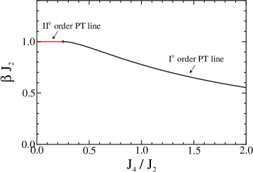
Figure 1: (Color online) $H_{2}+H_{4}$ case. Phase diagram in the ($J_{4}/J_{2},\beta J_{2}$) plane. Second and first order phase transition (PT) lines are reported.

$${\cal H}=-N\sum_{k=1}^{M}J_{2k}\ \rho^{2k}\ .$$ (8)

It is now possible to write the partition function

$${\cal Z}=\int d\{\varphi\}\ e^{-\beta{\cal H}}\ ,$$ (9)

as ktrig_pre :

$${\cal Z}\propto\int d\rho\ e^{-Ng(\rho;\beta)}\ ,$$ (10)

where $\beta=1/k_{B}T$ ($k_{B}$ is the Boltzmann constant, in the following we set $k_{B}=1$) and the function $g(\rho;\beta)$ is explicitly written as

$$g(\rho;\beta)=\beta\sum_{k=1}^{N}(2k-1)J_{2k}\rho^{2k}-\ln I_{o}\left(2\beta\sum_{k=1}^{M}kJ_{2k}\rho^{2k-1}\right)\ ,$$ (11)

where $I_{o}(x)$ is the modified Bessel function of order $0$.

Performing the thermodynamic limit $N\to\infty$, the saddle-point solution dominates the integral in (10). The saddle point equation is written as:

$$\rho=\frac{I_{1}(2\beta\sum_{k}kJ_{2k}\rho^{2k-1})}{I_{o}(2\beta\sum_{k}kJ_{2k}\rho^{2k-1})}\ .$$ (12)

This equation can have many solutions for $\rho$, that with the lowest free energy is the stable one

$$\beta f_{eq}(\beta)=\min_{\rho}g(\rho;\beta)\ .$$ (13)

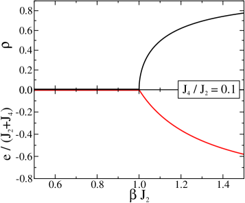
Figure 2: (Color online) $H_{2}+H_{4}$ case. Equilibrium magnetization $\rho$ (upper panel) and energy $e$ (rescaled by $J_{2}+J_{4}$, lower panel) as a function of inverse temperature $\beta$ (in unit of $J_{2}$) for $J_{4}/J_{2}=0.1$. Second-order phase transition takes place at $\beta J_{2}=1$.

Thermodynamic properties are obtained from the $\beta$-dependence of $g$. We note that the ”paramagnetic” ($\rho=0$) solutions always exist and is stable for small $\beta$ value. On increasing $\beta$ solutions with $\rho\neq 0$ becomes possible and, eventually, stable.

We note that for $J_{2}=0$ only first order phase transitions are possible. Indeed, in order to have a second order transition the curvature of the free energy, or of the function $g$, has to change around the paramagnetic solution $\rho=0$, from positive to negative. For $J_{2}>0$, close to $\rho=0$, we can expand Eq. (12) obtaining:

$$g\sim\beta J_{2}(1-\beta J_{2})\rho^{2}\ ,$$ (14)

then a second-order phase transition takes place at $\beta J_{2}=1$ (if not prevented by a first-order phase transition at higher temperature). For $J_{2}=0$ instead, denoting with $J_{p}$ the first non-zero term ($p\geq 4$), the expansion of Eq. (12) reads:

$$g\sim\beta J_{p}\rho^{p}\ ,$$ (15)

the curvature is always positive and then second-order transition cannot take place.

For a single term Hamiltonian ${\cal H}=H_{2k}$, the system undergoes second- ($k=1$) or first- ($k\geq 2$) order phase transition. We do not analyze these cases here, as the thermodynamic/topology relationship falls into the same class of similar model systems - $XY$ XY and $k$-trigonometric ktrig already discussed in the literature. We focus our attention in many-terms Hamiltonian, taking into account two interesting cases.

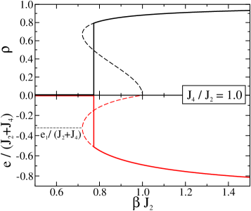
Figure 3: (Color online) $H_{2}+H_{4}$ case. Equilibrium (full lines) and metastable (dashed lines) magnetization $\rho$ (upper panel) and energy $e$ (rescaled by $J_{2}+J_{4}$, lower panel) as a function of inverse temperature $\beta$ (in unit of $J_{2}$) for $J_{4}/J_{2}=1.0$. A first-order phase transition takes place at $\beta J_{2}\simeq 0.77$. $e_{1}$ is the energy corresponding to the appearance of metastable free-energy states.

III.1 $H_{2}+H_{4}$ case

Considering the Hamiltonian ${\cal H}=H_{2}+H_{4}$, similarly to the corresponding Ising case Ising24 , the plane spanned by the two coupling parameters is split in two regions (see Fig. 1), which, as can be seen from Eq. 12, are only determined by the ratio $J_{4}/J_{2}$. Specifically,

i) For $J_{4}/J_{2}<1/4$ a second order phase transition takes place at $\beta J_{2}=1$. As an example, in Fig. 2 the equilibrium magnetization $\rho$ (upper panel) and energy per particle $e=-J_{2}\rho^{2}-J_{4}\rho^{4}$ (normalized by $J_{2}+J_{4}$, lower panel) are reported as a function of the (scaled) inverse temperature $\beta J_{2}$ for the specific case $J_{4}/J_{2}=0.1$.

ii) For $J_{4}/J_{2}>1/4$ the transition becomes first order, with a jump in both magnetization and energy - full lines in Fig. 3 where the same quantities as in Fig. 2 are reported for the specific case $J_{4}/J_{2}=1.0$. The dashed lines in Fig. 3 represent metastable states: metastable minimum of free energy for $e<e_{1}$ and local maximum for $e>e_{1}$.

For the particular case $J_{4}/J_{2}=1/4$ a tricritical point is present at $\beta J_{2}=1$.

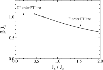
Figure 4: (Color online) $H_{2}+H_{6}$ case. Phase diagram in the ($J_{6}/J_{2},\beta J_{2}$) plane. Second and first order phase transition (PT) lines are reported.

III.2 $H_{2}+H_{6}$ case

The case ${\cal H}=H_{2}+H_{6}$ has a richer phenomenology (see Fig. 4).

i) For $J_{6}/J_{2}<0.46$ the system, similarly to the case $H_{2}+H_{4}$, undergoes a second order phase transition at $\beta J_{2}=1$. Fig. 5 reports, as an example, the order parameter and the energy as a function of the scaled temperature for the specific case $J_{6}/J_{2}=0.1$.

ii) For $0.46<J_{6}/J_{2}<0.66$ a first order phase transition occurs after (on increasing $\beta$, lowering $T$) the second order one (Fig. 6 reports the specific case $J_{6}/J_{2}=0.6$).

iii) For $J_{6}/J_{2}>0.66$ only the first order transition survives (Fig. 7 reports the specific case $J_{6}/J_{2}=1.0$).

The dashed lines in Fig.s 6 and 7 represent metastable states: metastable minima for $e<e_{1}$ and $e>e_{2}$ and local maximum for $e_{1}<e<e_{2}$.

IV Topology

In this Section we will study the topology of the two models introduced in the previous Section.

We will follow the same line of calculation performed on similar models in previous works ktrig ; ktrig_long ; modelock . A quantity directly related to the Euler characteristic of the manifold $M_{e}=\{\varphi|{\cal H}(\varphi)\leq Ne\}$, is the configurational entropy of saddles ktrig :

$$\sigma(e)=-n(e)\ln n(e)-(1-n(e))\ln(1-n(e))\ ,$$ (16)

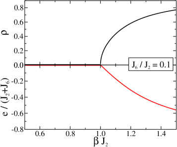
Figure 5: (Color online) $H_{2}+H_{6}$ case. Equilibrium magnetization $\rho$ (upper panel) and energy $e$ (normalized by $J_{2}+J_{6}$, lower panel) as a function of inverse temperature $\beta$ (in unit of $J_{2}$) for $J_{6}/J_{2}=0.1$. Second-order phase transition takes place at $\beta J_{2}=1$.

where $n(e)$ is the fractional saddle order (i.e. the fraction of negative curvatures at the saddle points that are found in the potential energy hyper-surface when $V(q)=Ne$). Indeed, we can make the following arguments.
A stationary point is defined by

$$\frac{\partial H}{\partial\varphi_{j}}=\sum_{k=1}^{M}2kJ_{2k}\ \rho^{2k-1}\sin(\varphi_{j}-\psi)=0\ \ \ \ \ \ \forall j$$ (17)

The solutions with $\rho>0$ (those with $\rho=0$ are located at $e=0$ energy) are obtained from $\sin(\varphi_{j}-\psi)=0$ (for all $j$), then

$$\varphi_{j}=\left[\psi+m_{j}\pi\right]_{{\rm mod}\ 2\pi}$$ (18)

where $m_{j}=\{0,1\}$. Substituting this solution in Eq. (7) we obtain

$$\rho=1-2n\ ,$$ (19)

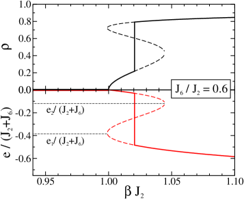
Figure 6: (Color online) $H_{2}+H_{6}$ case. Equilibrium (full lines) and metastable (dashed lines) magnetization $\rho$ (upper panel) and energy $e$ (normalized by $J_{2}+J_{6}$, lower panel) as a function of inverse temperature $\beta$ (in unit of $J_{2}$) for the specific case $J_{6}/J_{2}=0.6$. A second-order phase transition takes place at $\beta J_{2}=1$, followed by a first-order one at $\beta J_{2}\simeq 1.02$. $e_{1}$ and $e_{2}$ are the energies corresponding to the appearance of metastable free-energy states.

where

$$n=\frac{1}{N}\sum_{j}m_{j}$$ (20)

is the fractional saddle order (as it will be clear soon) and we have used the identity $(-1)^{m_{j}}=1-2m_{j}$. We conclude that there are no stationary points with $n>1/2$ ($\rho$ is positive defined). The order of a stationary point is defined by its downward curvatures, i.e. by the number of negative eigenvalues of the Hessian matrix $H_{ij}=\partial{{}^{2}H}/\partial{\varphi_{i}}\partial{\varphi_{j}}$. It is possible to show that in the thermodynamic limit the Hessian becomes diagonal

$$H_{ij}\simeq\delta_{ij}\ \lambda_{j}\ ,$$ (21)

where

$$\begin{split}\lambda_{j}&=\cos(\varphi_{j}-\psi)\ \sum_{k=1}^{M}2kJ_{2k}\ \rho^{2k-1}\\ &=(-1)^{m_{j}}\ \sum_{k=1}^{M}2kJ_{2k}\ \rho^{2k-1}\ .\end{split}$$ (22)

Therefore, the saddle order is given by the number of $m_{j}=1$ at the considered saddle point, and the fractional saddle order $n$ is then given by Eq. (20). Moreover, the number of saddles with a given $n$ is given by the binomial coefficient, then

$$\sigma(e)=\lim_{N\to\infty}\frac{1}{N}\ln\binom{N}{Nn(e)}\ ,$$ (23)

from which the Eq. (16) follows straightforward. The latter can be written in the form

$$\sigma(e)=-\frac{1-\rho(e)}{2}\ln\frac{1-\rho(e)}{2}-\frac{1+\rho(e)}{2}\ln\frac{1+\rho(e)}{2}\$$ (24)

where $\rho(e)$ is obtained from the thermodynamics, i.e. from the solution of the equation:

$$e=-\sum_{k=1}^{M}J_{2k}\ \rho^{2k}(e)$$ (25)

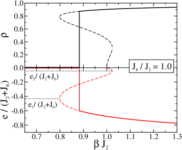
Figure 7: (Color online) $H_{2}+H_{6}$ case. Equilibrium (full lines) and metastable (dashed lines) magnetization $\rho$ (upper panel) and energy $e$ (normalized by $J_{2}+J_{6}$, lower panel) as a function of inverse temperature $\beta$ (in unit of $J_{2}$) for the specific case $J_{6}/J_{2}=1.0$. A first-order phase transition takes place at $\beta J_{2}\simeq 0.88$. $e_{1}$ and $e_{2}$ are the energies corresponding to the appearance of metastable free-energy states.

We note that the quantity $\sigma$ is singular at $e=0$, due to the fact that $e>0$ is a forbidden energy region, so $\sigma$ has a discontinuity, jumping from a finite value to zero.

As discussed in the introduction, a central quantity in the comparison between thermodynamic and topology is the curvature of $\sigma(e)$. Specifically, we are interested in finding the energy values where there is changes in curvature of $\sigma(e)$, i.e. the energies where the second derivative of $\sigma(e)$ vanishes. After some algebra we get

$$\frac{d^{2}\sigma}{de^{2}}=-\frac{1}{2}\left(\frac{d\rho}{de}\right)^{2}s[\rho(e)]\ ,$$ (26)

where the function $s$, which depends on $e$ through $\rho(e)$, is:

$$s(\rho)=\frac{1}{1-\rho}+\frac{1}{1+\rho}+\frac{\sum_{k}2k(2k-1)J_{2k}\rho^{2k-2}}{\sum_{k}2kJ_{2k}\rho^{2k-1}}\ln\frac{1-\rho}{1+\rho}$$ (27)

From Eq. 26 we have

$$s\lesseqgtr 0\;\Longleftrightarrow\;\frac{d^{2}\sigma}{de^{2}}\gtreqless 0\ ,$$ (28)

that is upward, null, downward curvature respectively. Studying the positivity of $s$ allows us to determine the curvature of $\sigma$. We now specialize the calculations to the two previous cases.

Figure 8: (Color online) $H_{2}+H_{4}$ case. (a) Saddle-entropy $\sigma$ as a function of energy $e$ (normalized by $J_{2}+J_{4}$) for $J_{4}/J_{2}=0.1,0.4,1.5$. Full (dashed) lines correspond to negative (positive) curvature. Symbols mark turning points. (b) Couplings-energy plane: light-grey region corresponds to $\sigma$ positive curvature, dark-grey region to entropy $S$ positive curvature. Dashed line is the inherent saddle counterpart of the border of dark region.

IV.1 $H_{2}+H_{4}$ case

In Fig. 8, upper panel, the quantity $\sigma(e)$ is plotted as a function of energy $e$ (normalized by $J_{2}+J_{4}$) for three selected case $J_{4}/J_{2}=0.1,0.4,1.5$. Full lines correspond to negative curvature, while dashed lines to positive (symbols represent turning points). In the $J_{4}/J_{2}=0.1$ case (second order phase transition located at $e=0$) the curvature is always negative, while in the other two both regions are present. The quantity $\sigma(e)$ is singular (discontinuous) at $e=0$, corresponding to the thermodynamic transition energy. In Fig. 8, lower panel, the plane $(J_{4}/J_{2},e)$ is drawn (the energy is normalized by $J_{2}+J_{4}$). The light-grey region corresponds to positive curvature of $\sigma(e)$, its border being the null curvature line - the correspondence with the turning points of $\sigma(e)$ in the upper panel of Fig. 8 is evidenced with the thin dashed lines for $J_{4}/J_{2}=0.4$ and $1.5$. The border of the light-grey region does not intersect the value $J_{4}/J_{2}=0.1$, and, therefore, no turning point exists for such a $J_{4}/J_{2}$ value.

The dark-grey region (that fully lies inside the light-grey one) represents the thermodynamically forbidden region $e>e_{1}$ (see Fig. 3). It corresponds to positive curvature of thermodynamic entropy $S(e)$. If the topological hypothesis was correct, the two, light- and dark-grey, regions would coincide. This is not the case, suggesting a not one-to-one correspondence between thermodynamic and saddle entropy.

In the study of other models 1d ; phi4 , when the energy of the topological change were not coincident with the energy of the phase transition, it was found that the “weak” topological hypothesis was correct. Indeed, it has been shown that the correspondence between topological change and phase transition energies were obtained considering inherent saddle properties: the energy of topology transition has been found to correspond to the inherent saddle energy. The latter quantity was obtained minimizing the quantity $W=|\nabla V|^{2}$ 1d ; ktrig_long ; sad_prl .

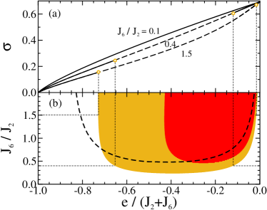
Figure 9: (Color online) $H_{2}+H_{6}$ case. (a) Saddle-entropy $\sigma$ as a function of energy $e$ (normalized by $J_{2}+J_{6}$) for the specific cases $J_{6}/J_{2}=0.1,0.4,1.5$. Full (dashed) lines correspond to negative (positive) curvature. Symbols mark turning points. (b) Couplings-energy plane: light-grey region corresponds to $\sigma$ positive curvature, dark-grey region to entropy $S$ positive curvature. Dashed line is the inherent saddle counterpart of the border of the dark-grey region.

Dashed line in Fig. 8b is the inherent saddle line obtained from the border of the dark-grey region (zero curvature thermodynamic entropy) applying the minimization procedure of $W$. The latter has been performed solving steepest descent equations of the form $\dot{\varphi}=-\nabla W$ starting from equilibrium initial configurations and taking at the end the infinite time limit. Following similar calculations of Ref. ktrig_long , we obtain the saddle energy $e_{s}=e(\rho_{\infty})$ where $\rho_{\infty}=L_{0}(-\beta de/d\rho)/I_{0}(-\beta de/d\rho)$ and $L_{0}$ is the modified Struve function of order $0$: $L_{0}(\alpha)=2\pi^{-1}\int_{0}^{\pi/2}d\varphi\sinh(\alpha\cos\varphi)$. A better correspondence is obtained between the light-grey border and the dashed line, however the two regions are not yet coincident. This indicates that the ”weak” topological hypothesis could only be considered a good approximation, but not a quantitative prescription for the location of the phase transitions. A comment is in order. Although obtained from canonical ensemble, the saddle energy map (from instantaneous to saddle energy) is expected to be ensemble-independent, when extrapolated to thermodinamically forbidden energy regions. “Ensemble inequivalence” phenomena eip are then supposed to not affect the results.

Summarizing: the singular behavior of $\sigma$ at $e=0$ signals the presence of a thermodynamic transition, the curvature of $\sigma$ is “quasi”-related to the presence of thermodynamically forbidden region and then to the appearance of a first-order transition. The “quasi”-relation is due to the fact that there are regions where the curvature of $\sigma$ is positive and the curvature of thermodynamic entropy is negative.

IV.2 $H_{2}+H_{6}$ case

In Fig. 9 the same as in the previous case is reported for ${\cal H}=H_{2}+H_{6}$. In the upper panel the energy dependence of $\sigma$ is reported for the specific cases $J_{6}/J_{2}=0.1,0.4,1.5$. As before, dashed lines correspond to positive curvature regions. In Fig. 9b the plane $(J_{6}/J_{2},e)$ is drawn: light-grey region is the $\sigma$-positive curvature, dark-grey one is the $S$-positive curvature. Dashed line is the inherent saddle counterpart of dark region border. Again, beside an overall qualitative behavior, we do not find a quantitative correspondence between the two regions that, according to the weak topological hypothesis, should coincide. We note that there are values of parameters ($0.2\lesssim J_{6}/J_{2}\lesssim 0.5$) where the curvature of $\sigma$ is upward (for certain energy values) and a second order transition takes place (the curvature of $S$ is downward).

V Conclusions

By analytically studying the thermodynamics and the topology of mean-field models obtained by the sum of two different interaction terms in the Hamiltonian (1) - $2+4$ and $2+6$ body terms - we are able to compare thermodynamic and topological quantities and test the validity of both the “topological hypothesis” cccp and the “weak topological hypothesis” 1d . The models have a rich phase space structure. The $H_{2}+H_{4}$ model performs second or first order phase transition depending on the coupling parameters values (a tricritical point joins the two). The $H_{2}+H_{6}$ model has a further possible behavior: it can undergo a double phase transition, a second order followed by a first order one. Topological invariant (saddle entropy) has a change in correspondence of the zero energy (the paramagnetic energy), so confirming in that case the equivalence between topological and thermodynamic transition points. However, only one topological change occurs, also for the $H_{2}+H_{6}$ model exhibiting two phase transition points. Indeed, in this case the first order phase transition does not have a topological counterpart, being the topological saddle entropy a smooth function at the corresponding phase transition energy values. It is worth noting that this is a quite unexpected result, all the models analyzed so far presenting a topological change at some energy value (even though not coincident with the phase transition one for some model system). Future studies should establish if this is a mean-field “pathology” or has a deeper origin. Moreover, the curvature of the saddle entropy (as a function of energy), seems not to be strictly related to the presence of first order phase transition (as previously observed in a different model ktrig ): there are regions in the parameters values for which positive curvature corresponds to second order phase transitions. In other words, the curvature properties of saddle entropy do not coincide with those of the thermodynamic entropy. Taking into account the possibility that the relevant energy levels are given by underlying saddles, a better agreement between curvature regions has been found, although there are no quantitative coincidence.

In conclusion, for the analyzed mean-field models a topology change is present at the same energy level at which a phase transition takes place, in agreement with the “topological hypothesis”. However, the information encoded in the topology seems not to be sufficient to predict all the possible thermodynamic behaviors of the system, like the presence of two phase transition points or the phase transition order.

References

- (1) L. Caiani, L. Casetti, C. Clementi, and M. Pettini, Phys. Rev. Lett. 79, 4361 (1997).
- (2) L. Casetti, M. Pettini, and E.G.D. Cohen, Phys. Rep. 337, 237 (2000).
- (3) M. Kastner, arXiv: cond-mat/0703401.
- (4) M. Pettini, Geometry And Topology in Hamiltonian Dynamics And Statistical Mechanics, Springer (2007).
- (5) R. Franzosi and M. Pettini, Phys. Rev. Lett. 92, 060601 (2004).
- (6) R. Franzosi, M. Pettini, and L. Spinelli, arXiv: math-ph/0505057.
- (7) R. Franzosi and M. Pettini, arXiv: math-ph/0505058.
- (8) R. Franzosi, M. Pettini, and L. Spinelli, Phys. Rev. Lett. 84, 2774 (2000).
- (9) S. Risau-Gusman, A.C. Ribeiro-Teixeira, and D.A. Stariolo, Phys. Rev. Lett. 95, 145702 (2005).
- (10) L. Casetti, M. Pettini, and E.G.D. Cohen, J. Stat. Phys. 111, 1091 (2003).
- (11) M. Kastner, Phys. Rev. Lett. 93, 150601 (2004).
- (12) P. Grinza and A. Mossa, Phys. Rev. Lett. 92, 158102 (2004).
- (13) A.C.R. Teixeira and D.A. Stariolo, Phys. Rev. E 70, 016113 (2004).
- (14) L. Angelani, L. Casetti, M. Pettini, G. Ruocco, and F. Zamponi, Europhys. Lett. 62, 775 (2003).
- (15) A. Andronico, L. Angelani, G. Ruocco, and F. Zamponi, Phys. Rev. E 70, 041101 (2004).
- (16) L. Angelani, G. Ruocco, and F. Zamponi, Phys. Rev. E 72, 06122 (2005).
- (17) M. Kastner, Physica A 365, 128 (2006).
- (18) L. Angelani, C. Conti, L. Prignano, G. Ruocco, and F. Zamponi, Phys. Rev. B 76, 064202 (2007).
- (19) L. Angelani, L. Casetti, M. Pettini, G. Ruocco, and F. Zamponi, Phys. Rev. E 71, 036152 (2005).
- (20) S. Velasco, J.A. White, and J. Guemez, American Journal of Physics 61, 554 (1993).
- (21) F. Zamponi, L. Angelani, L.F. Cugliandolo, J. Kurchan, and G. Ruocco, J. Phys. A: Math. Gen. 36, 8565 (2003).
- (22) L. Angelani, R. Di Leonardo, G. Ruocco, A. Scala, and F. Sciortino, Phys. Rev. Lett. 85, 5356 (2000).
- (23) J. Barrè, D. Mukamel, and S. Ruffo, Phys. Rev. Lett. 87, 030601 (2001).