The Faint and Extremely Red K-band Selected Galaxy Population in the DEEP2/Palomar Fields

Abstract

We present in this paper an analysis of the faint and red near-infrared selected galaxy population found in near-infrared imaging from the Palomar Observatory Wide-Field Infrared Survey. This survey covers 1.53 deg² to 5 $\sigma$ detection limits of K_vega = 20.5-21 and J_vega = 22.5, and overlaps with the DEEP2 spectroscopic redshift survey. We discuss the details of this NIR survey, including our J and K band counts. We show that the K-band galaxy population has a redshift distribution that varies with K-magnitude, with most K $<17$ galaxies at $z<1.5$ and a significant fraction (38.3$\pm 0.3$%) of $K>19$ systems at $z>1.5$. We further investigate the stellar masses and morphological properties of K-selected galaxies, particularly extremely red objects, as defined by $(R-K)>5.3$ and $(I-K)>4$. One of our conclusions is that the ERO selection is a good method for picking out galaxies at $z>1.2$, and within our magnitude limits, the most massive galaxies at these redshifts. The ERO limit finds 75% of all M${}_{*}>10^{11}$ M${}_{\odot}\,$galaxies at $z\sim 1.5$ down to K${}_{\rm vega}=19.7$. We further find that the morphological break-down of $K<19.7$ EROs is dominated by early-types (57$\pm 3$%) and peculiars (34$\pm 3$%). However, about a fourth of the early-types are distorted ellipticals, and within CAS parameter space these bridge the early-type and peculiar population, suggesting a morphological evolutionary sequence. We also investigate the use of a $(I-K)>4$ selection to locate EROs, finding that it selects galaxies at slightly higher average redshifts ($<z>=1.43\pm 0.32$) than the $(R-K)>5.3$ limit with $<z>=1.28\pm 0.23$. Finally, by using the redshift distribution of $K<20$ selected galaxies, and the properties of our EROs, we are able to rule out all monolithic collapse models for the formation of massive galaxies.

1 Introduction

Deep imaging and spectroscopic surveys in the optical have become the standard method for determining the evolution of the galaxy population (e.g., Kron 1980; Steidel & Hamilton 1993; Williams et al. 1996; Giavalisco et al. 2004). These surveys have revolutionised galaxy formation studies, and have allowed us to characterise basic properties of galaxies, such as their luminosity functions, stellar masses, and morphologies, and how these properties have evolved (e.g., Lilly et al. 1995; Ellis 1997; Wolf et al. 2003; Conselice et al. 2005a). However, due to technological limitations with near-infrared arrays, most deep surveys have been conducted in optical light, typically between $\lambda=$ 4000-8000 Å. This puts limits on the usefulness of optical surveys, as they select galaxies in the rest-frame ultraviolet at higher redshifts where many of the galaxies contributing to the faint end of optical counts are located (e.g., Ellis et al. 1996). Galaxies selected in the rest-frame ultraviolet limit our ability to trace the evolution of the galaxy population in terms of stellar masses. As the properties of galaxies can be quite different between the rest-frame optical and UV (e.g., Windhorst et al. 2002; Papovich et al. 2003, 2005; Taylor-Manger et al. 2006; Ravindranath et al. 2006), it is desirable to trace galaxy evolution at wavelengths where most of the stellar mass in galaxies is visible. To make advances in our understanding of galaxy evolution and formation at high redshifts, ($z>1$), therefore requires us to search for, and investigate, galaxy properties in the near-infrared (NIR).

Studying galaxies in the NIR has many advantages, including minimised K-corrections which are often substantial in the optical, as well as giving us a more direct probe of galaxy stellar mass up to $z\sim 3$ (e.g., Cowie et al. 1994). This has been recognised for many years, but most NIR surveys have been either deep pencil beam surveys (e.g., Gardner 1995; Djorgovski et al. 1995; Moustakas et al. 1997; Bershady, Lowenthal & Koo 1998; Dickinson et al. 2000; Saracco et al. 2001; Franx et al. 2003), or large-area, but shallow, surveys (e.g., Mobasher et al. 1986; Saracco et al. 1999; McCracken et al. 2000; Huang et al. 2001; Martini 2001; Drory et al. 2001; Elston et al. 2006). This is potentially a problem for understanding massive and evolved galaxies at high redshifts, as red objects are highly clustered (e.g., Daddi et al. 2000; Foucaud et al. 2007), as are the most massive galaxies (e.g., Coil et al. 2004a).

Previous deep NIR surveys can detect these unique galaxy populations, but they typically do not have a large enough area to probe the range of galaxies selected in the near-infrared. Likewise, large area, but shallow surveys may not be deep enough to detect with a high enough signal to noise these unique populations. In this paper we overcome this problem by presenting a 1.5 deg² survey down to 5 $\sigma$ depths of K_vega = 20.2-21.5 and J${}_{\rm vega}=22.5$. This brings together the properties of both deep and wide surveys. In this paper we explore NIR galaxy counts, and study the properties of faint NIR galaxies, which are often red in near-infrared/optical colours.

Unique galaxy populations have long been known to exist in near-infrared selected surveys. These include the extremely red objects (Elston, Reike, Reike 1988) and the distant red galaxies (Saracco et al. 2001; Franx et al. 2003; Conselice et al. 2007a; Foucaud et al. 2007), both of which are difficult to study at optical wavelengths. The existence of these galaxies reveals a large possible differential in the galaxy population between optical and near-infrared surveys. While these objects can be located in deep optical surveys, they are often very faint with $R>26$ (e.g., van Dokkum et al. 2006), making it difficult to understand these objects in any detail without NIR imaging or spectroscopy. In this paper we analyse the properties of galaxies selected in moderately deep K-band imaging. We also investigate the redshift distributions, structures and properties of the near-infrared selected galaxy population down to $K_{\rm vega}\sim 20$.

One of our main conclusions are that the faint K-band population spans a range of redshift and properties. We find that galaxies with magnitudes $K_{\rm vega}<17$ are nearly all at $z<1.4$. Galaxies with magnitudes $K_{\rm vega}=17-21$ are found at high redshift, up to at least $z\sim 4$. The colours of these galaxies span a wide range, with in particular redder galaxies seen at higher redshifts. Finally, we investigate the properties of the extremely red objects in our sample, finding that they include most, but not all of, the highest mass galaxies at $z\sim 1.5$. The morphologies of these EROs, and the redshift distribution and dust properties of $K_{\rm vega}<20$ sources, show that hierarchical galaxy formation is the dominate method by which massive galaxies form.

This paper is organised as follows: in §2 we discuss the data sources used in this paper, including our Palomar imaging, DEEP2 redshifts, and HST ACS imaging. This section also gives basic details of the Palomar survey. §3 includes our analysis, which contains information on the K and J-band counts, the redshift and colour distributions of K-selected galaxies. §4 includes an analysis of the extremely red galaxy population and its properties, including stellar mass, dust content, and redshift distributions. §5 includes a detailed discussion of our results in terms of galaxy models, while §6 is a summary of our findings. This paper uses Vega magnitudes unless otherwise specified, and assumes a cosmology with H${}_{0}=70$ km s^-1 Mpc^-1, $\Omega_{\rm m}=0.3$ and $\Omega_{\lambda}=0.7$.

2 Data, Reduction and Data Products

2.1 Data Sources

The objects we study in this paper consist of those found in the fields covered by the Palomar Observatory Wide-Field Infrared Survey (POWIR, Table 1). The POWIR survey was designed to obtain deep K-band and J-band data over a significant ($\sim$1.5 deg²) area. Observations were carried out between September 2002 and October 2005 over a total of $\sim 70$ nights. This survey covers the GOODS field North (Giavalisco et al. 2004; Bundy et al. 2005), the Extended Groth Strip (Davis et al. 2007), and three other fields the DEEP2 team has observed with the DEIMOS spectrograph (Davis et al. 2003). We however do not analyse the GOODS-North data in this paper given its much smaller area and deeper depth than the K-band imaging covering the DEEP2 fields. The total area we cover in the K-band in the DEEP2 fields is 5524 arcmin² = 1.53 deg², with half of this area imaged in the J-band. Our goal depth was K${}_{\rm vega}=21$, although not all fields are covered this deep, but all have 5 $\sigma$ depths between K = 20.2-21.5. Table 1 lists the DEEP2 fields, and the area we have covered in each. For our purposes we abbreviate the fields covered as: EGS (Extended Groth Strip), Field 2, Field 3, and Field 4.

The K-band data were acquired utilising the WIRC camera on the Palomar 5 meter telescope. WIRC has an effective field of view of $8.1\arcmin\times 8.1\arcmin$, with a pixel scale of 0.25″pixel^-1. In total, our K-band survey consists of 75 WIRC pointings. During observations of the K data we used 30 second integrations with four exposures per pointing. Longer exposure were utilised for the J-band data, with an exposure time of 120 seconds per pointing. Total exposure times in both K and J were between one to eight hours. The seeing FWHM in the K-band data ranges from 0.8” to 1.2”, and is on average 1.0”. Photometric calibration was carried out by referencing Persson standard stars during photometric conditions. The final K-band and J-band images were made by combining individual mosaics obtained over several nights. The K-band mosaics are comprised of co-additions of $4\times 30$ second exposures dithered over a non-repeating 7.0” pattern. The J-band mosaics were analysed in a similar way using single 120 second exposures per pointing. The images were processed using a double-pass reduction pipeline we developed specifically for WIRC. For galaxy detection and photometry we utilised the SExtractor package (Bertin & Arnouts 1996).

Photometric errors, and the K-band detection limit for each image were estimated by randomly inserting fake objects of known magnitude into each image, and then measuring photometry with the same detection parameters used for real objects. The inserted objects were given Gaussian profiles with a FWHM of 1$\aas@@fstack{\prime\prime}$3 to approximate the shape of slightly extended, distant galaxies. We also investigated the completeness and retrievability of magnitudes for exponential and de Vaucouleurs profiles of various sizes and magnitudes. A more detailed discussion of this is included in §2.4 and Conselice et al. (2007b).

Other data used in this paper consists of: optical imaging from the CFHT over all of the fields, imaging from the Advanced Camera for Surveys (ACS) on the Hubble Space Telescope, and spectroscopy from the DEIMOS spectrograph on the Keck II telescope (Davis et al. 2003). A summary of these ancillary data sets, which are mostly within the Extended Groth Strip, are presented in Davis et al. (2007).

The optical data from the CFHT 3.6-m includes imaging in the B, R and I bands taken with the CFH12K camera, which is a 12,288 $\times$ 8,192 pixel CCD mosaic with a pixel scale of 0.21″. The integration time for these observations are 1 hour in $B$ and $R$ and 2 hours in $I$, per pointing with 5 $\sigma$ depths of $\sim$ 25 in each band. For details of the data reduction see Coil et al. (2004b). From this imaging data a R_AB = 24.1 magnitude limit was used for determining targets for the DEEP2 spectroscopy. The details for how these imaging data were acquired and reduced, see Coil et al. (2004b).

The Keck spectra were obtained with the DEIMOS spectrograph (Faber et al. 2003) as part of the DEEP2 redshift survey. The EGS spectroscopic sample was selected based on a R-band magnitude limit only (with $R_{\rm AB}<24.1$), with no strong colour cuts applied to the selection. Objects in Fields 2-4 were selected for spectroscopy based on their position in $(B-K)$ vs. $(R-I)$ colour space, to locate galaxies at redshifts $z>0.7$. The total DEEP2 survey includes over 30,000 galaxies with a secure redshift, with about a third of these in the EGS field, and in total $\sim 11,000$ with a K-band detection (§3.1.1). In all fields the sampling rate for galaxies that meet the selection criteria is 60%.

The DEIMOS spectroscopy was obtained using the 1200 line/mm grating, with a resolution R $\sim 5000$ covering the wavelength range 6500 - 9100 Å. Redshifts were measured through an automatic method comparing templates to data, and we only utilise those redshifts measured when two or more lines were identified, providing very secure redshift measurements. Roughly 70% of all targeted objects resulted in reliably measured redshifts. Many of the redshift failures are galaxies at higher redshift, $z>1.5$ (Steidel et al. 2004), where the [OII] $\lambda$3727 lines leaves the optical window.

The ACS imaging over the EGS field covers a 10.1′$\times$ 70.5′  strip, for a coverage area of 0.2 deg². The ACS imaging is discussed in Lotz et al. (2006), and is briefly described here, and in Conselice et al. (2007a,b). The imaging consists of 63 titles imaged in both the F606W (V) and F814W (I) bands. The 5-$\sigma$ depths reached in these images are V = 26.23 (AB) and I = 27.52 (AB) for a point source, and about two magnitudes brighter for extended objects.

Our matching procedures for these catalogs progressed in the manner described in Bundy et al. (2006). The K-band catalog served as our reference catalog. We then matched the optical catalogs and spectroscopic catalogs to this, after correcting for any astrometry issues by referencing all systems to 2MASS stars. All magnitudes quoted in this paper are total magnitudes, while colours are measured through aperture magnitudes.

Table 1: The Palomar Fields, Number of WIRC pointings, and Area Covered

Field	RA	Dec.	# K	# J	K-area (arcmin2)
EGS	14 17 00	+52 30 00	33	10	2165
Field 2	16 52 00	+34 55 00	12	0	787
Field 3	23 30 00	+00 00 00	15	15	984
Field 4	02 30 00	+00 00 00	15	12	984
Total			75	37	4920

2.2 Photometric Redshifts

We calculate photometric redshifts for our K-selected galaxies, which do not have DEEP2 spectroscopy, in a number of ways. This sample is hereafter referred to as the ‘phot-z’ sample. Table 2 lists the number of spectroscopic and photometric redshifts within each of our K-band magnitude limits. These photometric redshifts are based on the optical+near infrared imaging, BRIJK (or BRIK for half the data) bands, and are fit in two ways, depending on the brightness of a galaxy in the optical. For galaxies that meet the spectroscopic criteria, $R_{\rm AB}<24.1$, we utilise a neural network photometric redshift technique to take advantage of the vast number of secure redshifts with similar photometric data. Most of the $R_{\rm AB}<24.1$ sources not targeted for spectroscopy should be within our redshift range of interest at $z<1.4$. The neural network fitting is done through the use of the ANNz (Collister & Lahav 2004) method and code. To train the code, we use the $\sim 5000$ redshifts in the EGS, which span our entire redshift range. The agreement between our photometric redshifts and our ANNz spectroscopic redshifts is very good using this technique, with $\delta z/z=0.07$ out to $z\sim 1.4$. The photometry we use for our photometric redshift measurements are done with a 2″  diameter aperture.

For galaxies which are fainter than $R_{\rm AB}=24.1$ we utilise photometric redshifts using two methods, depending on whether the galaxy is detected in all optical bands or not. For systems which are detected at all wavelengths we use the Bayesian approach from Benitez (2000). For an object to have a photometric redshift using this method requires it to be detected at the 3 $\sigma$ level in all optical and near-infrared (BRIJK) bands, which in the R-band reaches $\sim 25.1$. We refer to these objects as having ‘full’ photometric redshifts. As described in Bundy et al. (2006) we optimised our results and corrected for systematics through the comparison with spectroscopic redshifts, resulting in a redshift accuracy of $\delta z/z=0.17$ for $R_{\rm AB}>24.1$ systems. Further details about our photometric redshifts are presented in Conselice et al. (2007b), including a lengthy discussion of biases that are potentially present in the measured values.

Table 2 lists the number of galaxies with the various redshift types. As can be seen, the vast majority of our galaxies have either spectroscopic redshifts, or have measured photometric redshifts using the full optical SED. Only a small fraction ($<1$%) of our K-band sources are not detected in one optical band down to $K=21$.

For completeness in the analysis of the $N(z)$ distribution of K-magnitudes discussed in §5, we calculate, using a $\chi^{2}$ minimisation through hyper-z (Bolzonella, Miralles & Pello 2000), the best fitting photometric redshifts for these faint systems. These galaxies however make up only a small fraction of the total K-band population, and their detailed redshift distribution, while not likely as accurate as our other photometric redshifts, do not influence the results at all significantly.

2.3 Stellar Masses

From our K-band/optical catalogs we compute stellar masses based on the methods outlined in Bundy, Ellis, Conselice (2005) and Bundy et al. (2006). The basic method consists of fitting a grid of model SEDs constructed from Bruzual & Charlot (2003) stellar population synthesis models, with different star formation histories. We use an exponentially declining model to characterise the star formation history, with various ages, metallicities and dust contents included. These models are parameterised by an age, and an e-folding time for characterising the star formation history. We also investigated how these stellar masses would change using the newest stellar population synthesis models with the latest prescriptions for AGB stars from Bruzual & Charlot (2007, in prep). We found stellar masses that were only slightly less, by 0.07 dex, compared to the earlier models (see Conselice et al. 2007b for a detailed discussion of this and other stellar mass issues.)

Typical random errors for our stellar masses are 0.2 dex from the width of the probability distributions. There are also uncertainties from the choice of the IMF. Our stellar masses utilise the Chabrier (2003) IMF, which can be converted to Salpeter IMF stellar masses by adding 0.25 dex. There are additional random uncertainties due to photometric errors. The resulting stellar masses thus have a total random error of 0.2-0.3 dex, roughly a factor of two. However, using our method we find that stellar masses are roughly 10% of galaxy total masses at $z\sim 1$, showing their reliability (Conselice et al. 2005b). Details on the stellar masses we utilise, and how they are computed, are presented in Bundy et al. (2006) and Conselice et al. (2007b).

2.4 K-band Completeness Limit

Before we determine the properties of our K-selected galaxies, it is first important to characterise how our detection methods, and reduction procedures, influence the production of the final K-band catalog. While the major question we address is the nature of the faint and red galaxy population, it is important to understand what fraction of the faint population we are missing due to incompleteness. To understand this we investigate the K-band completeness of our sample in a number of ways. The first is through simulated detections of objects in our near-infrared imaging. As described in Bundy et al. (2006), Conselice et al. (2007b), and Trujillo et al. (2007) we placed artificial objects into our K-band images to determine how well we can retrieve and measure photometry for galaxies at a given magnitude. Our first simulations were performed from K = 18 to K = 22 using Gaussian profiles. We find that the completeness within our fields remains high at nearly all magnitudes, with a completeness of nearly 100% up to $K=19.5$ for all 75 fields combined together. The average completeness of these fields at $K=20$ is 94%, which drops to 70% at $K=20.5$ and 35% at $K=21.0$.

If we take the 23 deepest fields we find a completeness at $K=21.0$ of 70%. However, galaxies are unlikely to have Gaussian light profiles, and as such, we investigate how the completeness would change in Conselice et al. (2007b), if our simulations were carried out with exponential and r^1/4 light profiles. We find similar results as when using the Gaussian profiles up to $K=20$, but are less likely to detect faint galaxies with r^1/4 profiles, and retrieve their total light output. As discussed in §3.1.1, these incompleteness corrections are critical for obtaining accurate galaxy counts, but the intrinsic profiles of galaxies of interest must be known to carry this out properly. As such, we utilise the Gaussian corrections as a fiducial estimate. In Figure 1 we plot our K-band counts with these corrections applied. We also plot the J-band counts up to their completeness limit, and do not apply any corrections for incompleteness. The 100% completeness for the optical data is $B=25.25$, $R=24.75$, and $I=24.25$ (Coil et al. 2004b). These limits are discussed in §4.1 where we consider our ability to retrieve a well defined population of extremely red objects (EROs).

3 Analysis

3.1 Nature of the Faint K-band Population

3.1.1 K-band, J-band Counts and Incompleteness

Within our total K-band survey area of 1.53 deg² we detect 61,489 sources at all magnitudes, after removing false artifacts. Most of these objects (92%) are at K $<21$, while 68% are at K $<20$ and 37% are at K $<19$. In total there are 38,613 objects fainter than K $=19$ in our sample. Out of our total K-band population 10,693 objects (mostly galaxies) have secure spectroscopic DEIMOS redshifts from the DEEP2 redshift survey (Davis et al. 2003). We supplement these by 37,644 photometric redshifts within the range $0<z<2$ (Table 2). We remove stars from our catalogs, detected through their structures and colours, as described in Coil et al. (2005) and Conselice et al. (2007b).

Table 2: Number of K-band selected galaxies with various redshift measurements

K Range	Spec-z	Full Photo-z	Photo-z	Total
$15<K<17$	353	1541	1	1895
$17<K<19$	4305	11379	30	15714
$19<K<21$	5483	24405	215	30103

We plot the differential number counts (Table 3) for galaxies in both the K and J-band for our K-selected sample in Figure 1 to test how our counts compare with those found in previous deep and wide near-infrared surveys. We carry this out to determine the reliability of our star and galaxy separation methods, as well as for determining how our incompleteness corrections in the K-band compare to others. As Figure 1 shows, we find little difference in our counts compared to previous surveys, and we are $\sim$100% complete up to magnitude K$\sim 20$ in all fields. As others have noted, we find a change in the slope of the galaxy counts at K = 17.5. We calculate that the slope at $K<17.5$ is dN/dK = $0.54\pm 0.07$, while at $K>17.5$ it is dN/dK = $0.26\pm 0.01$.

Our counts, after correction, are slightly lower than those in the UKIDSS UDS survey (Simpson et al. 2006), and from studies by Cristobal-Hornillos et al. (2003) and Saracco et al. (1999). However, our counts are higher than those found in Iovino et al. (2005) and Kong et al. (2006). At brighter magnitudes these surveys all agree, with the exception of Maihara et al. (2001) who underpredict all surveys (not plotted). This difference at $K>20$ is likely the result of the different incompleteness correction methods used. As detailed in Bershady et al. (1998), using various intrinsic galaxy profiles when computing completeness can lead to over and underestimation of the correction factor. The only accurate way to determine the incompleteness is to know the detailed distribution of galaxy surface brightness profiles at the magnitude limits probed (Bershady et al. 1998). As this is difficult, and sometimes impossible to know, all corrected counts must be seen as best estimates.

Table 3: K-band and J-band Counts for all Fields

K-Magnitude	log N (deg-2 mag-1)	J-Magnitude	log N (deg-2 mag-1)
14.0	0.969${}^{+0.139}_{-0.206}$	14.5	1.074${}^{+0.176}_{-0.301}$
14.5	1.270${}^{+0.102}_{-0.135}$	15.0	0.949${}^{+0.198}_{-0.374}$
15.0	1.987${}^{+0.048}_{-0.054}$	15.5	0.949${}^{+0.198}_{-0.374}$
15.5	2.349${}^{+0.032}_{-0.035}$	16.0	1.852${}^{+0.081}_{-0.010}$
16.0	2.697${}^{+0.022}_{-0.023}$	16.5	2.265${}^{+0.052}_{-0.059}$
16.5	3.000${}^{+0.016}_{-0.016}$	17.0	2.540${}^{+0.038}_{-0.042}$
17.0	3.291${}^{+0.011}_{-0.011}$	17.5	2.847${}^{+0.027}_{-0.029}$
17.5	3.517${}^{+0.009}_{-0.009}$	18.0	3.152${}^{+0.019}_{-0.020}$
18.0	3.720${}^{+0.007}_{-0.007}$	18.5	3.370${}^{+0.015}_{-0.016}$
18.5	3.889${}^{+0.006}_{-0.006}$	19.0	3.631${}^{+0.011}_{-0.012}$
19.0	4.029${}^{+0.005}_{-0.005}$	19.5	3.840${}^{+0.008}_{-0.009}$
19.5	4.171${}^{+0.004}_{-0.004}$	20.0	4.004${}^{+0.007}_{-0.008}$
20.0	4.314${}^{+0.003}_{-0.004}$	20.5	4.185${}^{+0.006}_{-0.006}$
20.5	4.396${}^{+0.003}_{-0.003}$	21.0	4.288${}^{+0.005}_{-0.005}$
21.0	4.482${}^{+0.003}_{-0.003}$	21.5	4.315${}^{+0.005}_{-0.005}$

The J-band counts (Figure 1b) show a similar pattern as the K-band counts. These counts are not corrected for incompleteness and we are incomplete for very blue galaxies with $(J-K)<0$ at the faintest J-band limit due to our using the K-band detections as the basis for measuring J-band magnitudes. As can be seen, there is a larger variation in the J-band number counts when comparing the different surveys at a given magnitude compared to the K-band counts. Furthermore, there is no obvious slope change in the J-band counts, as seen in the K-band. We are complete overall in the J-band to J${}_{\rm vega}=22.0$ over the entire survey. Our J-band depth however varies between the three fields in which we have J-band coverage, and in fact varies between individual WIRC pointings.

As we later discuss the properties of EROs in this paper, as defined with a $(R-K)$ colour cut, it is important to understand the corresponding depths of the $R$-band imaging. The depth and number counts for the $R$-band imaging is discussed in detail in Coil et al. (2004b). Based on aperture magnitudes the 5 $\sigma$ depth of the CFHT R-band imaging is roughly $R_{\rm AB}=25$. Our $R$-band photometry uses the same imaging as Coil et al. (2004b), however we retrieved our own magnitudes based on the $K$-band selected objects in our survey. Our $R$-band depth however is similar to Coil et al. (2004b), and we calculate a 50% incompleteness at $R=25.1$.

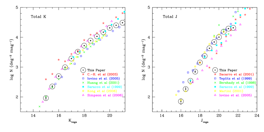
Figure 1: Differential K-band and J-band counts for our survey compared to previous published counts, including: Cristobal-Hornillos et al. (2003) (C.-H.), Huang et al. (2001), Saracco et al. (1999), Saracco et al. (2001), Teplitz et al. (1999), Bershady et al. (1998), Martini (2001), Kong et al. (2006), Iovino et al. (2005) and Simpson et al. (2006). Only the error bars are shown for the counts in our survey. The K-band counts at $K>20$ have been corrected for incompleteness, while the J-band counts are only shown to their completeness limit. At the faintest magnitudes the other surveys, with the exception of Simpson et al. (2006), have a larger error range due to the smaller areas used.

3.1.2 Redshift Distributions of K-Selected Galaxies

In this section we investigate the nature of galaxies selected in the K-band. The basic question we address is what are the properties of galaxies at various K-limits. This issue has been discussed earlier by Cimatti et al. (2002a), Somerville et al. (2004) and others. However, we are able to utilise the DEEP2 spectroscopic survey of these fields to determine the contribution of lower redshift galaxies to the K-band counts, and thus put limits on the contribution of high redshift $(z>1.5)$ galaxies to K-band counts at $K<20$.

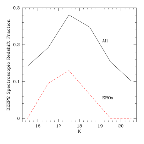
Figure 2: The spectroscopic redshift completeness for both the entire K-band selected catalog, and for the the $(R-K)>5.3$ ERO selected sample. Note that none of our EROs at $K>19.5$ have a measured spectroscopic redshift, typical for spectroscopic surveys which are optically selected.

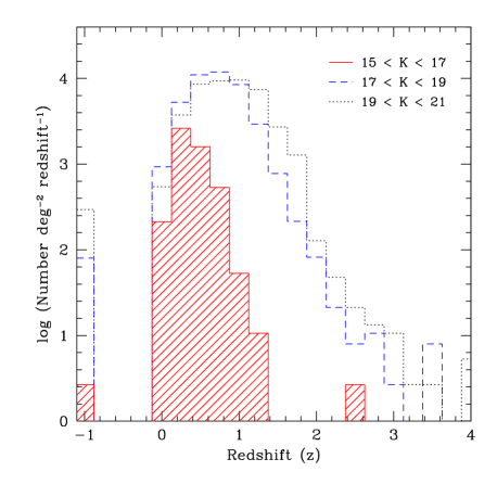
Figure 3: Redshift distributions for various K-band magnitude cuts. The solid black line shows the redshift distribution for all galaxies with $19<K<21$, the blued dashed line shows systems with $17<K<19$, and the red hashed histogram is for galaxies with $15<K<17$. The levels at $z=-1$ show the number of galaxies who had photo-zs not fit due to lacking significant optical detections.

The first, and most basic, method for understanding galaxies found in a K-band selection is to determine what fraction of the K-selected galaxies have a successfully measured spectroscopic redshift. The DEEP2 spectroscopic redshift success rate for our K-selected sample varies with K-band magnitude, from 10% to 30%, up to $K=21$. The highest selection fraction is 30% at K = 17.5. At the faintest limit, K = 21, the redshift selection is 10%, and the fraction is 15% at K = 15.5. Figure 2 shows our spectroscopic redshift completeness as a function of K-band magnitude for both the entire K-band selected sample, and the EROs (§4). The result of this plot is partially due to the fact that the DEEP2 selection deweights galaxies at $z<0.7$. The EGS and the other fields also have slightly different methods for choosing redshift targets (Davis et al. 2003), creating an inhomogeneous selection over the entire survey.

When we include photometric redshifts to supplement our spectroscopic redshifts, we obtain total redshift distributions shown in Figure 3. Note that our photometric redshifts are only included in Figure 3 at $z>0$ if the object was significantly detected in all bands in the BRIJK photometry. In each K-band limit shown in Figure 3, and discussed below, there are a fraction of sources which do not meet this optical criteria, and these objects are counted at the $z=-1$ position on the redshift histograms. In Table 2 we list the number of K-band detections with and without spectroscopic redshifts, in each of the redshift ranges.

It appears that nearly all bright K-band sources, with $15<K<17$, are located at $z<1.4$ (Figure 3). At fainter magnitudes, as shown by the plotted $17<K<19$ and $19<K<21$ ranges (Figure 3), we find a different distribution skewed toward high redshifts. While there are low redshift galaxies at these fainter K-limits, we also find a significant contribution of sources at higher redshifts, including those at $z>2$. The K-bright sources at these redshifts are potentially the highest mass galaxies in the early universe. Galaxies at the faintest magnitudes, at $19<K<21$, show a similar redshift distribution as the galaxies within the $17<K<19$ magnitude range, but there are a larger number of higher redshift galaxies. This demonstrates that faint K-band sources are just as likely to be at low redshift as at high redshift.

This is shown in another way using Figure 4 where we plot the distribution of K-magnitude vs. redshift ($z$). As can be seen, at $K>19$ the entire redshift range is sampled, while a $K<17$ selection only finds galaxies at $z<1.4$.

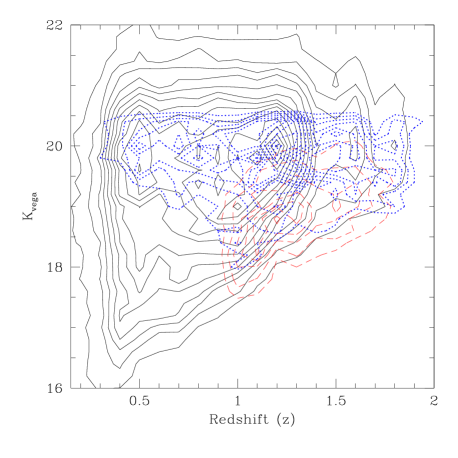
Figure 4: Contours of the redshift distribution for galaxies at various K-magnitudes. The red dashed contours are for EROs defined as (R-K)$>5.3$ (mostly at $z>1$), and the blue dotted contours are the distant red galaxies (DRGs) defined by $(J-K)>2.3$, which generally span $0.4<z<2$.

3.1.3 Colours of K-Selected Galaxies

After examining the redshift distribution of our sample, the next step is determining the physical features of these galaxies. The easiest, and most traditional, way to do this is through the examination of colour-magnitude diagrams. Generally, galaxy colour is a mixture of at least three effects - redshift, stellar populations and dust. Galaxies generally become redder with redshift due to band-shifting effects, and become redder with age, and increased dust content.

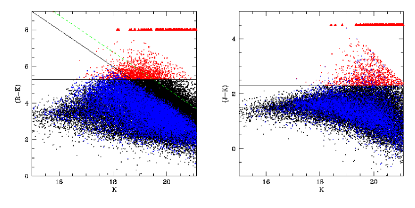
Figure 5: Colour-magnitude diagrams for our sample. The left panel shows (R-K) colour vs. K-band magnitude, while the right panel shows the (J-K) vs. K diagram. Objects with spectroscopic redshifts are coloured blue in both diagrams, while objects considered ‘red’ either through the extremely red objects (EROs) or Distant Red Galaxies (DRGs) selection are labelled as red in each diagram. The solid line in the (R-K) vs. K panel shows the spectroscopic limit of R = 24.1, while the dashed line shows the 5$\sigma$ limit for the R-band photometry of 25.1. Furthermore, we only plot points that are brighter than R = 26.5 and J = 23.5 in the two panels, respectively. The red triangles at the top of each figure are galaxies which are undetected in R or J, but have a measured K-band magnitude.

We can get an idea of the characteristics of our K-selected sample by examining the colour-magnitude diagram for the entire $K<21$ sample (Figure 5). Figure 5 plots the colours of our sample, as a function of $(B-R)$ and $(J-K)$ versus K-band magnitude. As can be seen, at fainter limits there are more red galaxies in each band. Since fainter/redder galaxies are more likely than brighter galaxies to be at higher redshifts, it is likely that these redder galaxies seen in Figure 5 are distant galaxies. The relation between $(R-K)$ and redshifts (Figure 6) shows this to be the case. As can be seen, at higher redshifts galaxies are redder in $(R-K)$, although even at these redshifts there are K-selected galaxies which are very blue. At the highest redshifts, where optical magnitudes are at $R>24$, we find that most galaxies hover around $(R-K)=5.3$. However, as can be seen, a significant fraction of the $K<19.7$ galaxies, which are massive systems at $z>1$, would be identified as EROs.

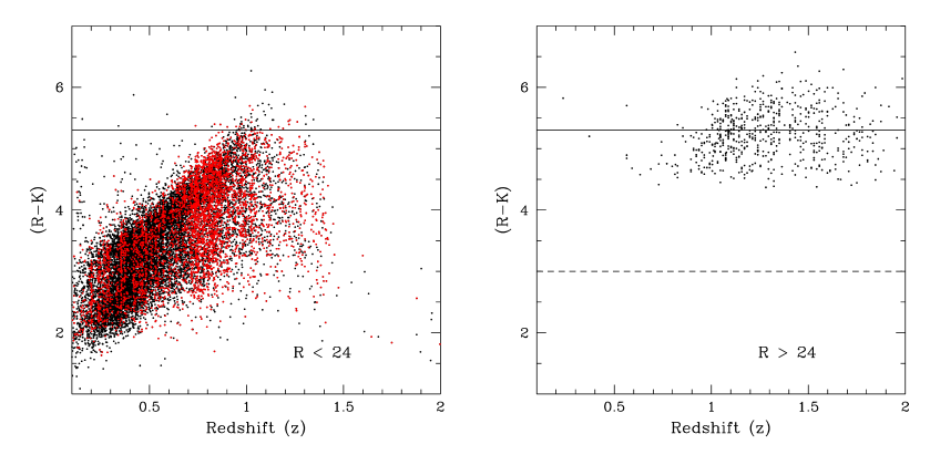
Figure 6: The redshift distribution for galaxies within our sample at $K<19.7$. The left panel shows systems which are at $R<24$. The right panel shows the distribution of $(R-K)$ colours as a function of redshift for galaxies which are fainter than $R=24$. As can be seen, galaxies generally get redder at higher redshifts, but there still exists a scatter in colour at any redshift.

The detailed distribution of magnitudes, colours and stellar masses is shown in Figure 7 and Figure 8, divided into different redshift bins. Plotted with different symbols are the photometric redshift and the spectroscopic redshift samples. As can been seen, there are strong relations between stellar mass and K-band magnitude over the entire redshift range (Figure 7), with fainter K-selected galaxies having lower stellar masses. Also note that the galaxies with spectroscopic redshifts are generally brighter and bluer than the photometric redshift sample at a given stellar mass. This is particularly true at the highest redshift bins, and demonstrates that the spectroscopy is successfully measuring the brighter galaxies in the distant universe, while being less efficient in measuring redshifts for galaxies of the same mass, but at a fainter K-magnitude.

Figure 8 furthermore shows how, as we go to higher redshifts, we obtain an overall redder distribution of colours. Within our lowest redshift bin, $0.5<z<0.75$, there are few galaxies which would be classified as EROs with $(R-K)>5.3$. It is also at this lowest redshift range where the overlap between the spectroscopic and photometric samples is highest. When we go to higher redshifts, such as at $0.75<z<1.0$, we find that the slope of the locus in the relation between stellar mass and $(R-K)$ colour steepens, such that galaxies at the same stellar mass become redder. This effect is dominated by the change in rest-frame wavelength sampled by the $R$ and $K$ filters. The fact that the higher mass galaxies become redder, while the lower mass galaxies tend to remain blue, is a sign that the spectral energy distributions of the lower mass galaxies are bluer than those for higher mass galaxies. This pattern evolves however, and at $z>1$, galaxies at every mass bin become redder with time. The upper envelope in the colour-stellar mass relation (Figure 8) is due to incompleteness, and is not a real limit.

On Figure 7 and Figure 8 we plot hydrodynamic simulation results from Nagamine et al. (2005) using different dust extinctions. We over-plot the E(B-V) = 0, 0.4 and 1 models on these figures as contours. First, the fact that there is not a larger scatter in the log M_∗ vs. $K$ relation (Figure 7) is an indication that these galaxies are not dominated by dust extinction. Very few galaxies overlap with the E(B-V) = 1 model, and most galaxies are better matched with the E(B-V) = 0 model. This can furthermore be seen in Figure 8 where only the lowest extinction model, with E(B-V) = 0, generally matches the location of galaxies in the $(R-K)$ vs. M_∗ diagram which are not EROs. The (E-V) = 0.4 model does a good job of tracing the EROs, but these systems could also be composed of old stellar populations. We revisit the issue of dust extinction in these galaxies in §5.1.

Finally, there are clearly two unique, and overlapping, samples identified in this near-infrared selected sample. The first are those galaxies in Figure 7 and 8 which are very massive, with masses M${}_{*}>10^{11}$ M${}_{\odot}\,$. We discuss these objects, and their evolution in Conselice et al. (2007b). We investigate in the next section the properties of the extremely red objects (EROs), those with observed colours, $(R-K)>5.3$.

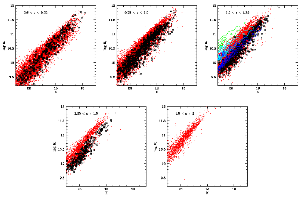
Figure 7: The stellar mass vs. K-band magnitude relation for our sample of galaxies out to $z\sim 2$. These figures are divided up into different redshifts, increasing from left to right and top to bottom. Plotted on these figures are both systems which have spectroscopically measured redshifts (open black boxes) and those which have photometric redshifts (the red dots). As can be seen, there is generally a strong relationship between stellar mass and apparent K-band magnitude, with a small scatter. Note that generally galaxies with spectroscopically measured redshifts are those which are brighter for a given stellar mass. These same systems are furthermore on the blue edge of the stellar mass-colour relationship (Figure 8). This shows that the DEEP2 spectroscopy is selecting primarily the bluer and brighter galaxies at a given stellar mass. We also plot in the $1.0<z<1.25$ bin models for how these quantities relate, from SPH simulations from Nagamine et al. (2005). The blue, cyan and green contours (going from low mass to high mass at a given K) show the location of model galaxies with E(B-V) = 0, 0.4 and 1, respectively.

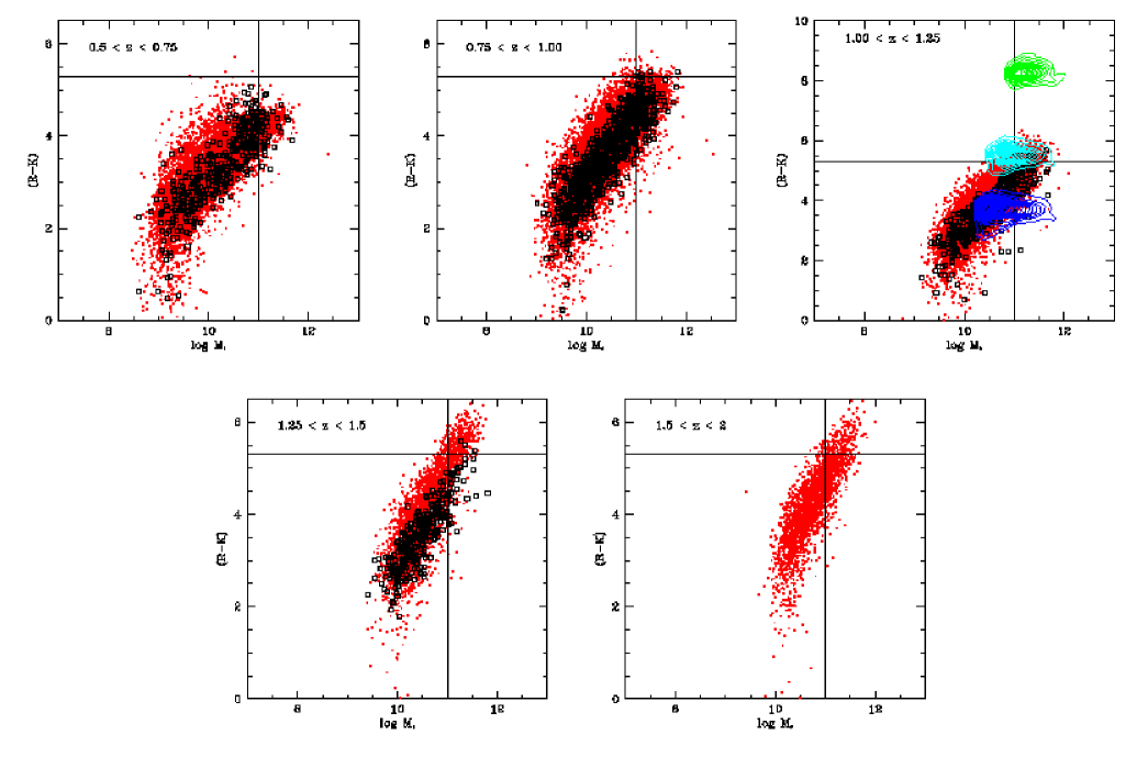
Figure 8: The colour-stellar mass relation for our sample to $z\sim 0$. Similar to Figure 7, these galaxies have been divided up into different redshift bins. The horizontal and vertical lines show the limits for selecting unique galaxy populations probed in the K-band. Galaxies to the right of the vertical line are massive galaxies studied in Conselice et al. (2007b), while galaxies which are above the horizontal line, defined by $(R-K)>5.3$ are the EROs studied in this paper. Note that the final redshift panel with $1.5<z<2.0$ consists solely of photometric redshifts. Also, similar to Figure 7 we plot in the $1.0<z<1.25$ figure models results from Nagamine et al. (2005), although we utilise the model results within the same limits as our data, $K<20$. As in Figure 7, the blue, cyan and green contours show the location of model galaxies with E(B-V) = 0, 0.4 and 1 (going from bluer to redder colours at a given stellar mass), respectively.

4 Properties of Extremely Red Objects

4.1 Sample Selection

The ERO sample we construct is defined through a traditional colour cut to locate the reddest galaxies selected in near infrared/optical surveys with $(R-K)>5.3$. Galaxies selected in this way are often considered the progenitors of today’s most massive galaxies, as seen at roughly $z\sim 1-2$. Objects with these extremely red colours have remained a population of interest since their initial discovery (Elson, Rieke & Rieke 1988). Initially thought to be ultra-high redshift galaxies with $z>6$, it is now largely believed that EROs are a mix of galaxy types at $z>1$ (e.g., Daddi et al. 2000; McCarthy et al. 2001; Firth et al. 2002; Smail et al. 2002; Roche et al. 2003; Cimatti et al. 2002; Yan & Thompson 2003; Cimatti et al. 2003; Moustakas et al. 2004; Daddi et al. 2004; Wilson et al. 2007). Generally, it has also been thought that EROs should trace some aspect of the massive galaxy population (Daddi et al. 2000); an idea we can test further with our data. Furthermore, because EROs are an easily defined and observationally based population, there has been considerable observation and theoretical work done towards understanding these objects. Naturally, it is more desirable to work with mass selected sample (see Conselice et al. 2007b for this approach), but these samples rely on accurate redshifts and stellar mass measurements, while the EROs are simply observationally defined through a colour.

The idea that EROs are red due to either an evolved galaxy population, or a dusty starburst is perhaps no longer the dominate way to think about these systems (e.g., Moustakas et al. 2004). However, there are properties of EROs that are still not understood, nor even constrained. For example, it is not clear why some EROs can have apparently normal galaxy morphologies, while others appear to be merging or peculiar galaxies (e.g., Yan & Thompson 2003; Moustakas et al. 2004).

The questions we address include: what are the stellar mass, morphological and redshift distributions for these objects? In our analysis we study the properties of these traditionally colour selected EROs to determine these basic properties.

Our sample of EROs however is not defined simply by a $(R-K)>5.3$ cut on our entire $R-$band and $K-$band catalogs. Due to the depth of both filters, we have to limit how deep we search for EROs to avoid false positives. As discussed in §2.4, we are 100% complete in our entire survey down to $K=20$. The $R-$band depth is however not well matched to the $K$-depth for finding EROs, and has a $>$ 5 $\sigma$ detection limit of $R=25.1$ (although 50% completeness). We therefore only select EROs which we are certain to within $>5$ $\sigma$ have a colour $(R-K)>5.3$. This limits our analysis of EROs down to $K=19.7$.

We divide our ERO sample into three types, depending on the origin of the redshift for each. The first type are those EROs with a high quality DEEP2 redshift, of which there are a total of 62 within our survey. The second type of ERO are those with $R<24.1$ which contain an ANNz photometric redshift (§2.2). There are 343 of these EROs. The third type are the EROs with magnitudes between $24.1<R<25.1$ which all have ‘full’ photometric redshifts (§2.2). There are 1122 of these objects. The entire $(R-K)>5.3$ sample therefore consists of 1527 EROs with some type of redshift. We examine the properties of $(I-K)>4$ selected EROs in §4.6.

4.2 ERO Number Counts

As with the number counts of the K-selected objects, we are interested in comparing the number counts of our ERO sample with measurements from previous work. In Figure 9 we plot the number counts for our ERO sample, as a function of K-magnitude. As can been seen, we are slightly under-dense at nearly all magnitudes compared to the UKIDSS UDS survey, but find similar results as Daddi et al. (2000). The differences between the counts in our survey and the UDS is likely due to several issues, including the slightly different filter sets used, and the correction for galactic extinction.

The UDS survey uses Subaru Deep Field imaging utilising the Cousins $R_{\rm C}$ filter, while our R-band imaging is from the CFHT and utilises a Mould R filter, which has different characteristics. Another issue is that these previous surveys have not corrected for Galactic extinction, while we have. This can result in slight differences in the number counts. Another feature seen in previous surveys, which we also see, is a turn-over in the slope of the counts at about K = 18.5, towards a shallower slope at fainter magnitudes.

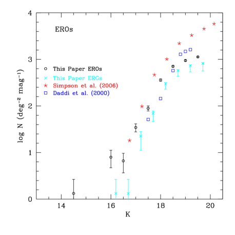
Figure 9: The number counts for EROs in our fields plotted along with the counts from previous surveys by Simpson et al. (2006) and Daddi et al. (2000). We also plot the number counts for the extremely red galaxies (ERGs) - the ERO counts with stars removed.

4.3 Redshift Distributions and Number Densities of EROs

One of principle quantities needed to understand the properties of EROs is their redshift distribution and number densities. With our three different types of redshifts (§2.2) measured for our EROs, we can construct the redshift distribution and number density evolution for EROs down to a magnitude limit of $K=19.7$. Figure 10a shows the redshift distribution for our $(R-K)>5.3$ selected EROs. We have plotted this distribution with three different histograms: for the spectroscopic redshift sample (red diagonal hatch), a photometric redshift sample for galaxies at $R_{\rm AB}<24.1$ (black), and a photometric redshift sample at $R_{\rm AB}>24.1$ (blue horizontal dashed).

It is clear that galaxies selected with the ERO criteria are at higher redshifts ($z>1$), with very few galaxies meeting this criteria at $z<0.8$, and all of those that do are photometrically derived redshifts. A similar pattern can be seen in Figure 6, which plots the colour-redshift distribution for our sample selected by $R_{\rm AB}<24$, and $R_{\rm AB}>24$.

The average redshift for our $K<19.7$ ERO sample is $<z>=$ 1.28$\pm$0.23. This is at a higher redshift and has a smaller dispersion than the average redshift for all galaxies with $K<19.7$, $<z>=0.84\pm 0.31$. The above arguments show that the traditional $(R-K)>5.3$ ERO cut reliably locates galaxies at $z>1$, on average. There is also a fairly long tail of sources up to $z\sim 2$.

Table 4: Extremely Red Object Number Densities for Systems at $K_{\rm vega}<19.7$.

ERO Selection	Redshift	log ($\phi$) (h${}^{3}_{70}$ Mpc-3 dex-1)
$(R-K)>5.3$	0.5	-6.00${}^{+0.31}_{-0.33}$
	0.7	-5.42${}^{+0.16}_{-0.27}$
	0.9	-4.64${}^{+0.10}_{-0.13}$
	1.1	-3.90${}^{+0.09}_{-0.11}$
	1.3	-4.10${}^{+0.09}_{-0.11}$
	1.5	-4.24${}^{+0.10}_{-0.11}$
	1.7	-4.70${}^{+0.14}_{-0.12}$
	1.9	-5.13${}^{+0.13}_{-0.15}$
$(I-K)>4$	0.5	-5.10${}^{+0.15}_{-0.23}$
	0.7	-5.19${}^{+0.14}_{-0.21}$
	0.9	-4.82${}^{+0.11}_{-0.14}$
	1.1	-4.16${}^{+0.09}_{-0.11}$
	1.3	-4.12${}^{+0.09}_{-0.11}$
	1.5	-4.11${}^{+0.10}_{-0.11}$
	1.7	-4.32${}^{+0.13}_{-0.11}$
	1.9	-4.47${}^{+0.11}_{-0.11}$

For the most part it appears that EROs at $K<19.7$ are selecting high redshift galaxies at $z\sim 1.3$. However, we are missing a few galaxies from our ERO sample at $K<19.7$ which do not have a redshift due to non-detections in the optical bands. These galaxies could be at very high redshift, and will be discussed in a future paper.

Figure 11 plots the number density evolution for our EROs at $K<19.7$ as a function of redshift, with tabulated values shown in Table 4. As can be seen, in agreement with Figure 10, there is a drop in the number density of EROs at $z<1$. The number density peak for EROs is also clearly found between $z=1-1.5$. We can compare this figure to previous measurements and models (e.g., Nagamine et al. 2005). Previously Moustakas et al. (2004) and Cimatti et al. (2002b) measured ERO number densities within various K-limits, but within $(R-K)>5$, as opposed to our $(R-K)>5.3$. However, when we compare our results to these papers, we find very similar results. Down to $K_{\rm vega}<20.12$, Moustakas et al. find a number density of EROs at $z=1$ of log($\phi$(Mpc^-3)) = $-3.19$, whereas we find $-3.39$ in roughly good agreement. Similarly, Cimatti et al. (2002b) find down to $K_{\rm vega}<19.2$ a density of log($\phi$(Mpc^-3)) = $-3.67$ at $z=1$, while we find $-3.60$, again in good agreement.

When we compare our results to simulation results from Nagamine et al. (2005) we find again roughly good agreement, although the Lagrangian SPH results find a slightly higher number density. At $z=1$ these SPH simulations find log($\phi$(Mpc^-3)) = $-2.96$, while the total variation diminishing (TVD) simulations give a slightly higher result. This density is a factor of 2.6 higher than the number density which we observe. These density are however the result of assuming a dust extinction of E(B-V) = 0.4, which might be too high in light of the results shown in Figures 7 and 8. Lower values of E(B-V) will make galaxies less red, and will produce a lower number density of EROs.

4.4 Stellar Masses of EROs

As shown in Figure 10b, our EROs generally have high stellar masses, and thus a fraction of the most massive galaxies at $z>0.8$ must be EROs. This is an important result, as it has been surmised from other criteria, such as clustering, that the EROs are contained within massive halos (e.g., Daddi et al. 2000; Roche, Dunlop & Almaini 2003).

We have constructed a complete sample of M${}_{*}>10^{11}$ M${}_{\odot}\,$galaxies up to $z\sim 1.4$ in our fields (Conselice et al. 2007b), from which we can directly test the idea that EROs are massive galaxies. Although Figure 10b demonstrates that our EROs at $K<19.7$ are selecting massive galaxies, this is likely due to the fact that our EROs are relatively bright, and we cannot constrain the masses or redshifts of fainter EROs, which must be either lower mass galaxies at the same redshifts as these, or higher redshift massive systems. There is also little difference in the distributions of stellar masses for our ERO sample at different redshifts. The peak mass is around 2$\times 10^{11}$ M${}_{\odot}\,$at all redshift selections.

We find that most of our sample of $K<19.7$ EROs tend to have masses M${}_{*}>10^{11}$ M${}_{\odot}\,$, which in the nearby universe are nearly all early-types (Conselice 2006a). This is a strong indication that $K<19.7$ EROs, regardless of their morphology or stellar population characteristics, are nearly certain to evolve into passive massive early-types in the nearby universe.

4.4.1 Are Massive Galaxies at $z>1$ EROs?

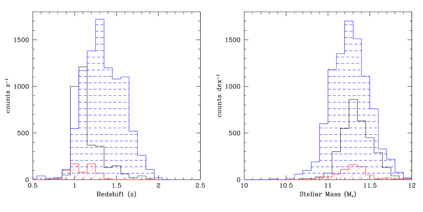
Figure 10: The redshift and stellar mass histograms for our sample of EROs. Shown are three histograms created after dividing the sample three different ways, depending on the origin of the redshift. The dotted diagonal hatched red histogram shows the redshift and stellar mass distributions for the spectroscopically confirmed EROs, while the non-hatched black histogram shows the distributions for EROs with $(R-K)>5.3$, $R_{\rm AB}<24.1$, and whose redshifts are photometric. The horizontal blue dashed hatched histogram shows the distributions for EROs with $R_{\rm AB}>24.1$ with measured photometric redshifts. As can be seen at a $K<19.7$ limit, the ERO selection generally locates massive galaxies at $z>1$.

While EROs are massive galaxies, the opposite of this is not necessarily true, as there are massive galaxies with M${}_{*}>$ $10^{11}$ M${}_{\odot}\,$, that are not EROs, some with very blue colours (Conselice et al. 2007b). Figure 12 plots the fraction of galaxies within the mass ranges M${}_{*}>$ $10^{11.5}$ M${}_{\odot}\,$and $10^{11}$ M${}_{\odot}\,$$<$ M${}_{*}<$ $10^{11.5}$ M${}_{\odot}\,$which are EROs between $z\sim 0-2$. Figure 11 plots the number density evolution for EROs selected in two ways and compares to galaxies selected with stellar masses M${}_{*}>$ $10^{11}$ M${}_{\odot}\,$. There are several interesting features in these figures. The first is that while massive galaxies exist throughout this redshift range, EROs only populate massive galaxies at $z>1$. Another interesting feature is that an ERO selection at $K<19.7$ will include a large fraction of the most massive galaxies with M${}_{*}>$ $10^{11.5}$ M${}_{\odot}\,$, at $1<z<2$. On average, between $1.0<z<1.4$, our ERO selection will find 36% of all M${}_{*}>$ $10^{11.5}$ M${}_{\odot}\,$galaxies. This increases to 75% within the redshift range $1.2<z<1.8$.

However, the ERO colour limit does not do a good job in selecting massive galaxies with $10^{11}$ M${}_{\odot}\,$$<$ M${}_{*}<$ $10^{11.5}$ M${}_{\odot}\,$. In this mass range at $1.0<z<1.4$ the ERO selection finds only 35% of these systems. Similar to the M${}_{*}>$ $10^{11.5}$ M${}_{\odot}\,$mass range, we find a higher fraction of $10^{11}$ M${}_{\odot}\,$$<$ M${}_{*}<$ $10^{11.5}$ M${}_{\odot}\,$galaxies which are EROs at 44%. However, with a $K<19.7$ limit, we are obtaining a similar number density of EROs per co-moving volume as there are massive galaxies (Figure 11). The number densities of EROs however declines rapidly at $z<1$.

While it appears that the traditional $(R-K)>5.3$ limit will find the most massive galaxies at $z>1$, this colour cut does not give a purely ultra-high mass sample, nor does it include all of the massive galaxies at these redshifts. At $1.2<z<1.8$ about 25% of galaxies with M${}_{*}>$ $10^{11.5}$ M${}_{\odot}\,$and 66% of systems with $10^{11}$ M${}_{\odot}\,$$<$ M${}_{*}<$ $10^{11.5}$ M${}_{\odot}\,$are not EROs. This is consistent with our finding in Conselice et al. (2007b) that $\sim 40$% of massive galaxies at $z>1$ are undergoing star formation and have blue $(U-B)_{0}$ colours.

4.5 Structural Features

We utilise visual estimates of Hubble types and the non-parametric CAS system to characterise the morphologies and structures of an ERO sample selected with $(R-K)>5$. While there are slightly more systems at $(R-K)>5.3$ than at $5<(R-K)<5.3$, we reduce our limit to aquire more systems for analysis and to better compare with previous work. A similar analysis is the focus of Conselice et al. (2007a,b), in which we examined the morphological properties of the most massive galaxies at $z>1.5$, as well as the Distant Red Galaxies (DRG), with $(J-K)>2.3$, which are also proposed to be the progenitors of today’s massive galaxies.

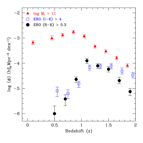
Figure 11: The co-moving number densities of EROs selected by the $(R-K)_{\rm vega}>5.3$ and the $(I-K)_{\rm vega}>4$ criteria as a function of redshift. Also plotted for reference is the number density evolution for galaxies with stellar masses M${}_{*}>$ $10^{11}$ M${}_{\odot}\,$(see Conselice et al. 2007b).

The CAS (concentration, asymmetry, clumpiness) parameters are a non-parametric method for measuring the structures of galaxies on CCD images (e.g., Conselice 2007; Conselice et al. 2000a,b; Bershady et al. 2000; Conselice et al. 2002; Conselice 2003). The basic idea is that low redshift, nearby galaxies, have light distributions that reveal their past and present formation modes (Conselice 2003). Furthermore, well-known galaxy types in the nearby universe fall in well defined regions of the CAS parameter space (Conselice 2003). We apply the CAS system to our EROs to determine their structural features. There are two caveats to using the ACS imaging on these galaxies. The first is that there are redshift effects which will change the measured parameters, such that the asymmetry and clumpiness indices will decrease (Conselice et al. 2000a; Conselice 2003), and the concentration index will be less reliable (Conselice 2003). There is also the issue that for systems at $z>1.3$ we are viewing these galaxies in their rest-frame ultraviolet images, which means that there are complications when comparing their measured structures with the rest-frame optical calibration indices for the nearby galaxies. Our main purpose in using the CAS system is to identify relaxed massive ellipticals as well as any galaxies that are still involved in a recent major merger and are presumably dusty.

The following structural and morphological analysis is based on the ACS imaging of the EGS field described in §2.1. The imaging we use covers 0.2 deg² in the F814W (I) band, giving us coverage for $\sim 15$% of our ERO sample.

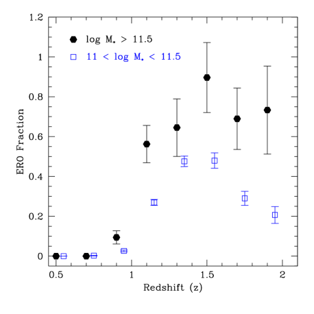
Figure 12: Diagram showing the fraction of galaxies with extreme masses M${}_{*}>$ $10^{11.5}$ M${}_{\odot}\,$(solid circles) and $10^{11}$ M${}_{\odot}\,$$<$ M${}_{*}<$ $10^{11.5}$ M${}_{\odot}\,$(open boxes) which are also $(R-K)>5.3$ selected EROs. As can be seen, the ERO selection successfully finds galaxies at $z>1$, yet does not locate all of these systems. A sample of EROs at $K<19.7$ will contain nearly all of the log M${}_{*}>11.5$ systems at $z\sim 1.5$, but is less successful at finding the lower mass, log M${}_{*}>11$ systems.

4.5.1 Eye-Ball/Classical Morphologies

We study the structures and morphologies of our sample using two different methods. The first is through simple visual estimate of morphologies based on the appearance of our ERO sample in CCD imaging. The outline of this process is given in Conselice et al. (2005a) and is also described in the companion paper (Conselice et al. 2007b). Our total sample of objects gives 436 unique EROs for which there is ACS imaging. Each of these galaxies were placed into one of six categories: compact, elliptical, lenticular (S0), early-type disk, late-type disk, edge-on disk, merger/peculiar, and unknown/too-faint. These classifications are very simple, and are only based on appearance. No other information, such as colour or redshift, was used to determine these types. An outline of these types is provided below, with the number in each class listed at the end of each description.

1. Ellipticals: A centrally concentrated galaxy with no evidence for a lower surface brightness, outer structure (152 systems). An additional 58 galaxies were classified as peculiar ellipticals, which appear similar to ellipticals, but have an unusual light distribution, or bulk asymmetry (see Conselice et al. 2007b).

2. Lenticular (S0): A galaxy was classified as an S0 if it appears as an elliptical but contained a disk-like outer structure with no evidence for spiral arms, or clumpy star forming knots or other asymmetries. (13 systems)

3. Compact - A galaxy was classified as compact if its structure was resolved, and is very similar to the elliptical classification in that these systems must be very smooth and symmetric. A compact galaxy differs from an elliptical in that it contain no obvious features, such as an extended light distribution or envelope. (24 systems)

4. Early-type disks: If a galaxy contained a central concentration with some evidence for lower surface brightness outer light, it was classified as an early-type disk. (3 systems)

5. Late-type disks: Late-type disks are galaxies that appear to have more outer low surface brightness light than inner concentrated light. (1 systems)

6. Edge-on disks: disk systems seen edge-on and whose face-on morphology cannot be determined but is presumably S0 or disk. (17 systems)

8. Peculiars/irregulars: Peculiars are systems that appear to be disturbed or peculiar looking, including elongated/tailed sources. These galaxies are possibly in some phase of a merger (Conselice et al. 2003a,b) and are common at high redshifts. (148 systems)

9. Unknown/too-faint: If a galaxy was too faint for any reliable classification it was placed in this category. Often these galaxies appear as smudges without any structure. These could be disks or ellipticals, but their extreme faintness precludes a reliable classification. (20 systems)

4.5.2 Morphological Distributions

The morphological distribution of the EROs can help us address the question of the origin of these extremely red galaxies. In the past, this technique has been used to determine the fraction of EROs which are early-type, disk or peculiar. Previous studies on this topic include Yan & Soifer (2003) who study 115 EROs, and Moustakas et al. (2004) who studied 275 EROs in the GOODS fields. Our total population of EROs for which we have morphologies is 436. These earlier studies have found a mix of types, with generally half of the EROs early-types, and the other half appearing as star forming systems in the form of disks or peculiars/irregulars.

In summary, we find that 57$\pm$3% of our EROs are early-type systems. This includes 58 systems, or 13% of the total, which are disturbed ellipticals. In classifications carried out in previous work some of these systems would be classified as peculiars. The bulk of the rest of the population consists of bonafide peculiars, which make up 34$\pm$3% of the ERO population. Only four EROs were found to be face on disk galaxies, while 17 systems (4%) of the ERO sample are made up of edge-on disk galaxies. Presumably these galaxies are red for different reasons - either evolved galaxy populations, or dusty star formation, or from dust absorption produced through orientation in the case of edge-on disks.

Previous work has been somewhat inconsistent on the morphological break-down between peculiars and early-type galaxies (e.g., Yan & Soifer 2003; Moustakas et al. 2004). From our study, it is clear that much of this difference can be accounted for by the peculiar ellipticals. These systems appear in their large-scale morphology to be early-type, but have unusual features, such as offset nuclei that make them appear peculiar. The differences between previous findings can largely be accounted for by whether these peculiar ellipticals were included in the early-type or peculiar class.

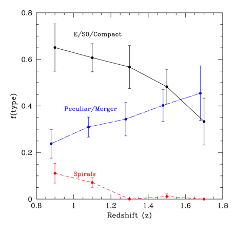
Figure 13: Our visual estimates of ERO morphological type as a function of redshift. As labelled, the ellipticals, S0s and compact morphological types are shown as a solid black line. The systems classified as a peculiar/mergers are shown as the dotted blue line and spirals are shown as the dashed red line.

We find that the relative number of peculiar and early-type EROs changes with redshifts (Figure 13), such that at the lowest redshifts ($z\sim 0.7$) the EROs are dominated by the E/S0/Compacts, with a type fraction of $\sim 65$%, but at $z>1.4$ the peculiar systems are more prominent. The fraction of EROs which are peculiars evolves from $\sim 45$% at $z\sim 1.7$ to $\sim 20$% at $z=0.9$. This mix between early types and peculiars evolves with redshift, although the exact reason for this evolution is not immediately clear. It is possible that some of the peculiars at $z>1.2$ only appear so because we are sampling their morphologies below the Balmer break that would produce more irregular/peculiar looking galaxies at these redshifts (Windhorst et al. 2002; Manger-Taylor et al. 2006; Conselice et al. 2007b). However, we are nearly always probing the rest-frame optical where the effects of the morphological k-correction are minimised both qualitatively and quantitatively (e.g., Conselice et al. 2005a; Conselice et al. 2007c in prep). We also find a higher fraction of peculiar systems within the ERO sample, than what is found for massive galaxies with M${}_{*}>$ $10^{11}$ M${}_{\odot}\,$at similar redshifts (Conselice et al. 2007b).

Interestingly, we find that 10-15% of EROs at $z\sim 0.9$ are spiral/disks. For the most part however, it appears that most of the EROs are ellipticals, but we find that peculiars make up roughly a third of the systems, with the relative contribution coming from galaxies at the highest redshifts. We discuss the morphological break-down of these systems in §5.2 in terms of models of galaxy formation and evolution.

4.5.3 CAS Structural Parameters

Another way to understand the structures of these systems is through their quantitative structural parameters as measured through the CAS system. The CAS parameters have a well-defined range of values and are computed using simple techniques. The concentration index is the logarithm of the ratio of the radius containing 80% of the light in a galaxy to the radius which contains 20% of the light (Bershady et al. 2000). The range in $C$ values is found from 2 to 5, with higher $C$ values for more concentrated galaxies, such as massive early types. The asymmetry is measured by rotating a galaxy’s image by 180${}^{\circ}\,$and subtracting this rotated image from the original galaxy’s image. The residuals of this subtraction are compared with the original galaxy’s flux to obtain a ratio of asymmetric light. The radii and centreing involved in this computation are well-defined and explained in Conselice et al. (2000a). The asymmetry ranges from 0 to $\sim 1$ with merging galaxies typically found at $A>0.35$. The clumpiness is defined in a similar way to the asymmetry, except that the amount of light in high frequency ‘clumps’ is compared to the galaxy’s total light (Conselice 2003). The values for $S$ range from 0 to $>2$, with most star forming galaxies having values, $S>0.3$.

We show in Figure 14 the CA and AS projection of CAS space for EROs defined by $(R-K)>5$. As can be seen, the EROs, which are mostly early-types and peculiars, as defined by eye (Figure 14), fall along a large portion of the range of possible values in CAS space. As expected, the irregulars/peculiars have higher asymmetries, lower concentrations, and higher clumpiness values than the early types. This is similar to, but not exactly the same, as the structural parameter distribution for the most massive galaxies with M${}_{*}>$ $10^{11}$ M${}_{\odot}\,$at $z<1.4$. There is a larger fraction of peculiars within the ERO sample, and the redshift evolution with types is not identical between EROs and massive galaxies (cf. Conselice et al. 2007b).

As with the massive galaxies found at high redshifts, the ERO visually determined types are slightly higher in asymmetry than their $z\sim 0$ counterparts (Conselice 2003). Figure 14 shows how the EROs classified as early-types have slightly larger asymmetries than their visual morphology would suggest. The distorted early-types have even higher asymmetries on average. Most systems also deviate from the asymmetry-clumpiness relation (Figure 14), showing that the production of these asymmetries is more likely due to dynamical effects, rather than star formation (Conselice 2003). Interestingly, we find that many of the peculiar EROs do not have a high clumpiness index, which is opposite to what we found for high asymmetry systems within the massive galaxies sample (Conselice et al. 2007b). The reason for this is that these red galaxies are likely dusty, and therefore bright star clusters are not seen within the ongoing star formation. This furthermore shows that the EROs are likely more dominated by galaxy merging than a pure mass selected sample.

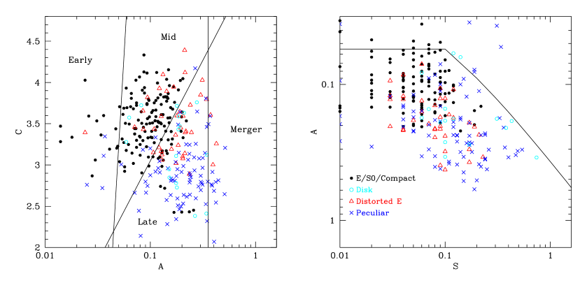
Figure 14: The CAS space for our ERO sample with $(R-K)>5$. Objects are labelled by their visual classification, discussed in §4.5.1. The solid black symbols represent the normal (non-distorted) ellipticals, S0s and compacts. The open red triangles are the distorted ellipticals, while the blue crosses are galaxies classified as peculiars/mergers, and the open cyan circles are for the few disk galaxies found within the ERO sample.

We can understand the origin of these morphologies, and how they relate to the origin of the EROs, by comparing the CAS parameters of the EROs to their stellar masses. Figure 15 shows the comparison between ERO asymmetries and concentrations vs. their stellar masses. The concentration-stellar mass diagram shows a few interesting trends. The most obvious feature is that there appears to be a broad bimodality between EROs which are peculiar, and those which are early-types.

The peculiars and early-types have similar masses, typically M${}_{*}\sim 10^{11}$ M${}_{\odot}\,$, yet they have different light concentrations. The peculiars typically have lower concentrations, $C=2-3$, while the early-types are generally at $C>3$. The early-types also tend to show a correlation between concentration and stellar mass which is not seen for the peculiars. The distorted ellipticals fall in between these two populations suggesting an evolutionary connection in the passive evolution of galaxy structure. What we are potentially witnessing is the gradual transition from peculiar EROs at high redshifts, to passive ellipticals at lower redshifts, while on the way going through a distorted elliptical stage. This is consistent with the idea that the $z=1-2$ epoch is where massive galaxies final reach their passive morphology (Conselice et al. 2003; Conselice et al. 2005; Conselice 2006).

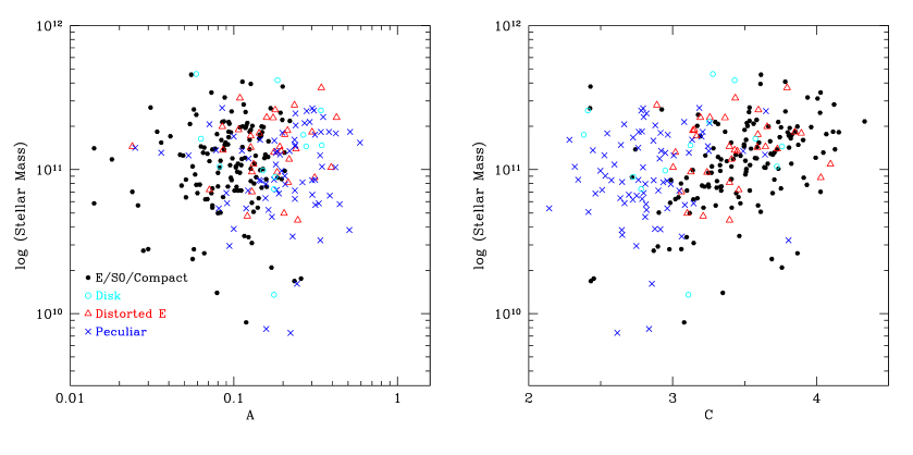
Figure 15: The relationship between asymmetries and light concentrations of our ACS EROs with their stellar masses. The symbols for each type are the same as in Figure 14. There appears to be a remarkable bimodal distribution in these parameter spaces such that peculiars have low light concentration and higher asymmetries than the elliptical-like objects, while having similar stellar masses. The distorted ellipticals appear to fall in the gap between these two populations, and are likely a transitional phase between the two. This can be seen furthermore in Figure 13 where the fraction of early-type EROs increases at the expense of the peculiars.

There also appears to be a bimodality within the stellar mass/asymmetry diagram (Figure 15). The peculiars in general have higher asymmetries than the early-types, but with the distorted ellipticals containing asymmetries mid-way between the peculiars and the ellipticals, suggesting again that the distorted ellipticals are a mid-way point in the evolution between the peculiar EROs and the passive EROs. As we do not see much mass evolution in the upper edge of the ERO mass distribution, it is likely that the peculiars are within their final merger phase, and transform into early-types relatively quickly over $1<z<2$. A similar pattern can be seen for a high mass selected sample of galaxies at similar redshifts (Conselice et al. 2007b).

4.6 Other ERO Selection Criteria

ERO selection through the $(R-K)>5.3$ criteria is only one way to find extremely red objects. Another popular method for finding EROs is a selection with $(I-K)>4$ (e.g., Moustakas et al. 1997). While both of these selection methods are used to find EROs, it is not clear how these two methods compare, and whether they are finding the same galaxy population. We investigate this issue briefly in this section.

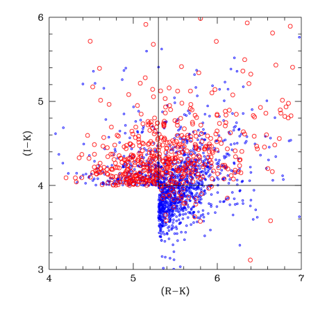
Figure 16: The $(I-K)$ vs. $(R-K)$ diagram for galaxies in our sample. Only shown are those galaxies which are considered EROs either through the $(R-K)>5.3$, or the $(I-K)>4$ criteria. The points are plotted in terms of their redshifts, with galaxies at $z>1.5$ shown as open red circles and galaxies at $z<1.5$ as blue dots. The $(I-K)>4$ limit appears to find galaxies at higher redshifts, on average, than the $(R-K)>5.3$ limit.

Figure 16 shows the relationship between $(I-K)$ and $(R-K)$ colours for galaxies within our sample. Those objects which have photometric redshifts $z>1.5$ are plotted as the red open symbols, while those at $z<1.5$ are plotted as the blue dots. What is obvious from this figure is that an ERO selection with $(I-K)>4$ is more likely to pick out galaxies at higher redshifts than the $(R-K)>5.3$ limit. This limit also appears to contain more contamination from lower redshift galaxies than the $(R-K)>5.3$ limit. Overall, we find an overlap of 767 EROs through both definitions down to $K=19.7$, this overlap constitutes 54% of the $(R-K)>5.3$ EROs and 60% of the $(I-K)>4$ EROs.

In Figure 17 we show the redshift distribution for the EROs selected with $(I-K)>4$, which can be directly compared with the redshift distribution for $(R-K)>5.3$ systems in Figure 10. As can be seen, the redshift distribution for the $(I-K)>4$ systems is skewed towards higher redshifts than the $(R-K)>5.3$ selection. We find that, on average, the redshifts for the $(I-K)>4$ EROs is $<$z$>$ = 1.43$\pm 0.32$, compared with $<$z$>$ = $1.28\pm 0.23$ for EROs selected with the $(R-K)>5.3$ limit. There are also fewer systems at $z<1.4$ within the $(I-K)>4$ selection than for the $(R-K)>5.3$ limit, suggesting that the redder bands are finding galaxies at slightly higher redshifts. However, this does not appear to be the case for the $(J-K)>2.3$ ‘distant red galaxies’ (DRGs), as discussed in Conselice et al. (2007a) and Foucaud et al. (2007). It appears that these systems are picking up a significant fraction of massive galaxies at $z\sim 1$ up to $K=20$.

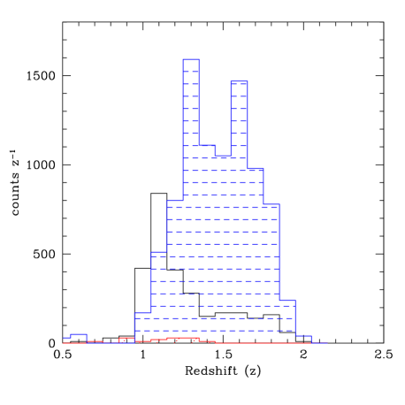
Figure 17: Similar to Figure 10, but for ERO systems which have been selected with the $(I-K)>4$ limit. As can be seen by comparing this figure with Figure 10, we are selecting, on average, higher redshift galaxies with these redder bands.

5 Discussion

Here we discuss the results from this paper in the context of galaxy formation models and scenarios. We include in this discussion the redshift distribution of K-selected galaxies, as well as the stellar mass and structural/morphological properties of EROs to address how the stellar mass assembly of galaxies is likely taking place. By examining these galaxies we are not relying on assumptions about stellar masses to find the most massive and evolved galaxies at high redshift. In this sense a K-band selected and colour selected population are an alternative approach from stellar mass selection (Conselice et al. 2007b) for understanding galaxy formation due to the simplicity, and reproducibility, of their selection.

We first examine the redshift distribution of $K<20$ galaxies, and compare this to models. We use colour information of our faint K-selected galaxies to rule out all monolithic collapse formation scenarios for galaxies. We then examine the properties of the EROs themselves to further argue that these systems are, due to their stellar masses, likely an intrinsically homogeneous population, with the peculiar EROs evolving into the ellipticals at lower redshifts.

5.1 K-band Redshift Distributions

The number of K-band selected galaxies per redshift at a given K-magnitude limit is an important test of when the stellar masses of galaxies were put into place. In general, ideas for how massive galaxies form explicitly predict how much stellar mass galaxies would have in the past. In a rapid formation, such as with a monolithic collapse, the stellar mass for the most massive galaxies, which in a K-band limited sample will always probe the massive systems, the number of galaxies within a bright K-band limit, say $K<20$ at high redshift should be much larger than the number of sources seen in a hierarchical model, which predicts that the stellar masses of galaxies grows with time. Therefore the number of bright galaxies at higher redshifts in a hierarchical model is less than that predicted in a monolithic collapse. This test was first performed by Kauffmann & Charlot (1998) who concluded, based on an early hierarchical model, that the predicted counts exceed the observations, a result which has remained despite improvements in data and models (e.g., Kitzbichler & White 2006).

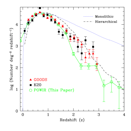
Figure 18: Redshift distribution of our sample with a $K<20$ cut. Comparisons to previous redshift distributions published in the K20 and GOODS surveys are shown. The two lines demonstrate predictions of fiducial monolithic collapse (Kitzbichler & White 2006), and hierarchical model predictions (Kitzbichler & White 2007) for this evolution within the same K-band limit.

In Figure 18 we show the number of $K<20$ galaxies as a function of redshift for systems at $z<4$. We further plot on Figure 18 model predictions for how $N(z)$ changes in a standard pure luminosity evolution monolithic collapse model from Kitzbichler & White (2006), and within a standard hierarchical formation scenario from Kitzbichler & White (2007). We have used in this figure our entire K-band distribution, including galaxies for which we had to measure photometric redshifts without an optical band (§2.2). We also plot on Figure 18 the $K<20$ magnitude distribution for galaxies seen in the GOODS and K20 surveys.

While we generally agree with these previous results, we find a slightly lower number of systems at higher redshifts compared to GOODS and K20. The reason for this could simply be cosmic variance, as the GOODS and K20 samples at these redshifts also differ by a large amount. Otherwise, this difference is likely created by errors within our photometric redshifts. However, it must be noted that the integrated number of $K<20$ galaxies is similar for our survey and GOODS and K20, but is still much smaller than that predicted by the monolithic model.

As can be seen in Figure 18 there is clearly a large difference between the observed distribution, and the predicted monolithic collapse distribution. We can rule out this basic monolithic collapse model, which does not include dust, at $>$ 10 $\sigma$, based on the comparisons to our $K<20$ redshift distribution. It is possible to match with a monolithic collapse model if extreme dust content is included in these galaxies, or if there are ‘hidden’ galaxies (Kitzbichler & White 2006). However, as we argue below, there is no evidence that dusty galaxies dominate our K-band selected sample.

From Figure 18 it appears that a basic hierarchical model agrees better with the data (e.g., Somerville et al. 2004; Stanford et al. 2004; Kitzbichler & White 2007). There is perhaps a slight excess of galaxies in the hierarchical formation model, which has been noted before (e.g., Kauffman & Charlot 1998; Somerville et al. 2004; Kitzbichler & White 2007). The origin of this difference is not clear. It perhaps simply implies that too much mass is produced early in the hierarchical model, yet this would seem to contradict the fact that the most massive galaxies with M${}_{*}>$ $10^{11}$ M${}_{\odot}\,$are nearly all in place by $z\sim 1.5-2$ (Conselice et al. 2007b). We address this apparent conflict in more detail in §5.2.

Although the basic hierarchical model agrees better with the observed redshift distribution, there are scenarios where the monolithic model can fit the data as well as the hierarchical scenario (see also Cimatti et al. 2002a). These scenarios require that the K-band selected galaxies have a significant amount of dust extinction in the observed K-band. The amount of extinction needed varies from 1.0 to 0.7 mag at rest-frame $z$ and $R$ bands from $z=1.5-2$ (Kitzbichler & White 2006). This extinction needed is even higher at $z=1-1.5$.

By using the colours of galaxies that fit within the $K<20$ criteria, we can determine what the contribution of dusty galaxies are to these counts. Stellar population synthesis models show that only old stellar populations, and galaxies with dust extinctions with A${}_{\rm v}>1$, have a colour of $(R-K)>5$ at $z=1-4$. We can use this information, and the model results using various dust extinctions from Nagamine et al. (2005) (Figures 7 and 8), to argue that these galaxies are not dominated by dust extinction, which would need to be the case to reconcile the observed K-band distribution with a monolithic collapse model.

First, the model results compared to data shown in Figures 7 and 8, and discussed in §4.3 clearly show that K-selected galaxies are not dominated by heavy dust extinction. At best, only models with E(B-V) = $0-0.4$ are able to reproduce the location of real galaxies. The E(B-V) = 0.4 models are however even too red to account for most galaxies in the $(R-K)$ vs. M_∗ diagram (Figure 8). A representative value of R_V = A_V/E(B-V) = 3.1 reveals values of A${}_{\rm V}=0-1.28$ for this range in E(B-V). For the Calzetti et al. (2000) extinction law, this gives lower values, with A${}_{\rm V}=0-0.25$. Thus, it does not appear likely that our $K<20$ galaxy sample is dominated by enough dust extinction (A${}_{\rm V}=1$ needed, on average) to match the monolithic collapse galaxy count model.

We find that only 28.3$\pm 0.6$% of $K<20$ selected galaxies at $1<z<2$ have a colour $(R-K)>5$, required to meet the minimum condition for dust extinction. We have further argued in §4, that a significant fraction of these EROs are old passively evolving stellar populations, which are unlikely to have a screen of dust with A${}_{\rm V}>1$ (see e.g., White, Keel & Conselice 2000). As discussed in §4.5.2 over half of the EROs at $1<z<2$ appear as early-types, thus at most only $\sim 14\%$ of the $K<20$ galaxies at $1<z<2$ have a significant amount of dust extinction. The dusty pure-luminosity evolution monolithic collapse models from Kitzbichler & White (2006) predict that all $K<20$ galaxies have this amount of dust extinction, which clearly they do not. It is thus impossible to reconcile the K-band redshift distribution with any monolithic model.

In summary our K-band redshift distribution, and those from the K20 and GOODS surveys, appear to be much closer to the basic hierarchical model of Kitzbichler & White (2007) than to the monolithic collapse model. We can also rule out pure luminosity evolution models with significant dust extinction. Therefore, down to $K=20$ at $z<4$ it appears that the monolithic model cannot be the dominate method for forming galaxies.

5.2 Structural Evolution

As discussed in §4.5, a large fraction of the EROs we have HST imaging appear to be undergoing some type of evolution based on their structural appearance. A logical conclusion is that many of the peculiar systems are in some phase of a merger (Conselice et al. 2003a). We can quantify this by examining the merger fraction as derived through the CAS definition of $A>0.35$ and $A>S$ (Conselice 2003). This is a strict definition, and will allow us to measure a lower limit on the merger fraction, even when observing in the rest-frame ultraviolet (Taylor-Mager et al. 2007).

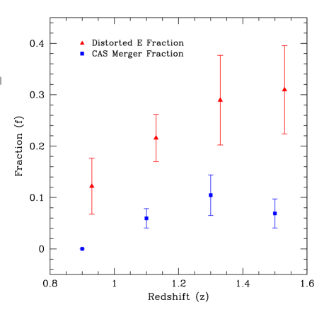
Figure 19: The fraction of galaxies identifiable as a merger using the CAS system, and the fraction of early-types which appear to have a distorted structure.

Figure 19 shows the evolution of the merger fraction derived through this CAS definition. We also include the fraction of early-types which appear to have a distorted structure. It appears from this that between $5-10\%$ of the EROs at $1<z<2$ would be identified as a major merger through the CAS parameters. This is a factor of $\sim 3$ less than the peculiar fraction (Figure 13), which is what we would expect for a population which is undergoing major mergers (Conselice 2006; Bridge et al. 2007). The reason for this is that the CAS approach is sensitive to $\sim 0.4$ Gyr of the merger process (Conselice 2006), while eye-ball estimates of merging last for $\sim 1.2$ Gyr (Conselice 2006). This is another indication that the peculiar galaxies we are seeing in the ERO population are in fact undergoing merging.

Figure 20, as well as Figure 15 demonstrate what evolution is likely occurring within the ERO population. As can be seen, the EROs, within our $K<19.7$ selection, have the same upper range of masses at $z\sim 0.8-2$ (Figure 20). Therefore, little mass growth occurs within this population at this K-band limit. We also know that a large fraction of the EROs with M${}_{*}>$ $10^{11}$ M${}_{\odot}\,$are peculiar in some way. This varies from 64$\pm$24% at $z>1.5$ to 41$\pm$6% at $1<z<1.25$ (§4.5). However, at $z\sim 0$ the fraction of M${}_{*}>$ $10^{11}$ M${}_{\odot}\,$red galaxies which are morphologically early-types is $\sim 85$% (Conselice 2006a; Conselice et al. 2007b).

It is clear that a significant fraction of EROs must have undergone morphological evolution as they cannot lose mass. What likely is occurring is that the distorted elliptical and peculiar galaxies which dominate the population at $z>1.5$ (Figure 13 and 20) transform into morphologically and spectrally evolved systems at $z\sim 1$. The reason this is likely the case is that there is no difference in the masses of the peculiar and the early-type EROs. This also explains why this population, despite having a mixed morphology clusters so strongly (e.g., Daddi et al. 2000; Roch et al. 2003). Calculations based on the merger rate in Conselice et al. (2007b) for the most massive galaxies suggest that on average about one or two major mergers are occurring for the M${}_{*}>$ $10^{11}$ M${}_{\odot}\,$population at $z<2$, but fewer at lower redshifts.

Finally, these major mergers are what may make the K-band counts in the hierarchical model redshift distribution higher than the observed. The reason is that in the standard hierarchical model, the number and mass densities of the most massive galaxies with M${}_{*}>$ $10^{11}$ M${}_{\odot}\,$underpredict the observed number of massive systems by up to two orders of magnitude (Conselice et al. 2007b). Within these models the stellar masses for these systems are largely already formed, but are in distinct galaxies that have not yet merged (De Lucia et al. 2006). It is thus easy to see that if a single massive galaxy at $z\sim 1.5$ was in several pieces, all of which would still meet the criteria of $K<20$ based on the relation of stellar mass and K-mag (Figure 7), then the number of galaxies with $K<20$ at higher redshift in the hierarchical model would be higher than the observed number. This is consistent with the number densities of massive galaxies being higher than in the models, as well as for a rapid formation of massive systems through major mergers at $z>2$ (Conselice 2006b).

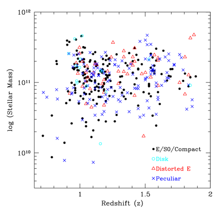
Figure 20: The distribution of ERO galaxy mass with redshift. Labeled on this figure are the morphological types for each galaxy as determined through our ACS imaging. Note that massive EROs are detected all the way out to $z=2$.

6 Summary

In this paper we analyse the faint K-band selected galaxy population as found in the Palomar NIR survey/DEEP2 spectroscopic survey overlap. Our primary goal is to determine the nature of the faint $K>19$ galaxy population. While many of these galaxies are too faint for detailed spectroscopy, we can investigate their nature through spectroscopic and photometric redshifts, stellar masses, as well as photometric and structural features. Our major findings include:

1. The redshift distribution for K-selected galaxies depends strongly on apparent K-magnitude. Most systems at $K<17$ are at $z<1.4$, while a significant fraction of sources with $17<K<19$ are at $z>2$. These K-bright high$-z$ galaxies are the progenitors of today’s massive galaxies.

2. We find that a significant fraction (28.3$\pm 0.6$%) of the $K<20$ galaxy population consists of extremely red or massive galaxies at $z>1$. We characterise the population of log M${}_{*}>11$ sources in Conselice et al. (2007b), while we analyse the extremely red objects (EROs) in this paper.

3. We find that EROs at $K<19.7$ are a well defined population in terms of redshifts and masses. Nearly all EROs are at $z>1$, and have stellar masses with M${}_{*}>10^{11}$ M${}_{\odot}\,$. EROs are therefore certainly the progenitors of today’s massive galaxies. The corollary to this however is not necessarily true. There are massive galaxies at $z>1$ that would not be selected with the ERO criteria. We find that the ERO selection locates 35-75% of all ultra-massive, M${}_{*}>10^{11.5}$ M${}_{\odot}\,$galaxies, at $z=1-2$, while only 25% of $10^{11}$ M${}_{\odot}\,$$<$ M${}_{*}<10^{11.5}$ M${}_{\odot}\,$galaxies are located with this colour cut.

4. We examine the morphological and structural properties of our ERO sample and find, as others previously have, a mixed population of ellipticals and peculiars. In total, we find that the ERO population is dominated by early-type galaxies, with an overall fraction of 57$\pm 3$% of the total. Interestingly, we find that a significant fraction of the early-types ($\sim 25$%) are distorted ellipticals, which could be classified as peculiars, although these systems at a slightly lower resolution than ACS, or using a quantitative approach would be seen as early-types. Peculiars account for the remaining 34%, and many of these are likely in some merger phase. This fraction tends to evolve such that the peculiars are the dominant population at higher redshifts, $z>1$.

5. We investigate the structural parameters for our EROs using the CAS system. We find that visual estimates of galaxy class and position in CAS space roughly agree, although the asymmetries of these systems are higher than what their visual morphologies would suggest. We find a bimodality in the stellar mass-concentration diagram where the peculiar EROs are at a low concentration and the early-types are highly concentrated. The distorted ellipticals fall in between these two populations suggesting an evolutionary connection in the passive evolution of galaxy structure within the ERO population.

6. We compare the $(R-K)>5.3$ ERO selection with the $(I-K)>4$ ERO selection, and find that the $(I-K)>4$ ERO are at slightly higher redshifts than the $(R-K)>5.3$ selection, suggesting that it is a more useful criteria for finding evolved galaxies at $z>1.5$.

7. By examining the redshift distribution of $K<20$ galaxies, and comparing to monolithic collapse and hierarchical formation models, we are able to rule out all monolithic collapse models for the formation of massive galaxies. These monolithic collapse models predict a higher number of $K<20$ galaxies as a function of redshift at a significance of $\sim 10$ $\sigma$. While some monolithic collapse models are able to reproduce our galaxy counts, these are dominated by dust. We are however able to show that only $\sim 14$% of the $K<20$ galaxies have potentially enough dust to match this model, the others being evolved galaxies, or blue star forming systems.

The Palomar and DEEP2 surveys would not have been completed without the active help of the staff at the Palomar and Keck observatories. We particularly thank Richard Ellis and Sandy Faber for advice and their participation in these surveys. We thank Ken Nagamine and Manfred Kitzbichler for providing their models and comments on this paper. We also thank the referee for their careful reading and commenting on this paper. We acknowledge funding to support this effort from a National Science Foundation Astronomy & Astrophysics Fellowship, grants from the UK Particle Physics and Astronomy Research Council (PPARC), Support for the ACS imaging of the EGS in GO program 10134 was provided by NASA through NASA grant HST-G0-10134.13-A from the Space Telescope Science Institute, which is operated by the Association of Universities for Research in Astronomy, Inc., under NASA contract NAS 5-26555. JAN is supported by NASA through Hubble Fellowship grant HF-01182.01-A/HF-011065.01-A. The authors also wish to recognise and acknowledge the very significant cultural role and reverence that the summit of Mauna Kea has always had within the indigenous Hawaiian community. We are most fortunate to have the opportunity to conduct observations from this mountain.

References

- (1) Benitez, N. 2000, ApJ, 536, 571
- (2) Bershady, M.A., Lowenthal, J.D., & Koo, D.C. 1998, ApJ, 505, 50
- (3) Bershady, M.A., Jangren, J.A., Conselice, C.J. 2000, AJ, 119, 2645
- (4) Bertin, E., Arnouts, S. 1996, A&AS, 117, 393
- (5) Bolzonella, M., Miralles, J.-M., & Pello, R. 2000, A&A, 363, 476
- (6) Bridge, C., et al. 2007, ApJ, 659, 931
- (7) Bundy, K., et al. 2006, ApJ, 651, 120
- (8) Bundy, K., Ellis, R.S., Conselice, C.J. 2005, ApJ, 625, 621
- (9) Calzetti, D., Armus, L., Bohlin, R.C., Kinney, A.L., Koornneef, J., Storchi-Bergmann, T. 2000, ApJ, 533, 682
- (10) Cimatti, A., et al. 2002, A&A, 391, 1L
- (11) Cimatti, A., et al. 2003, A&A, 412, 1L
- (12) Cristobal-Hornillos, D., et al. 2003, ApJ, 595, 71
- (13) Coil, A.L., et al. 2004a, ApJ, 609, 525
- (14) Coil, A.L., et al. 2004b, ApJ, 617, 765
- (15) Collister, A.A., Lahav, O. 2004, PASP, 116, 345
- (16) Conselice, C.J. 1997, PASP, 109, 1251
- (17) Conselice, C.J., Bershady, M.A., Jangren, A. 2000a, ApJ, 529, 886
- (18) Conselice, C.J. 2003, ApJS, 147, 1
- (19) Conselice, C.J., Bershady, M.A., Dickinson, M., Papovich, C. 2003a, AJ, 126, 1183
- (20) Conselice, C.J., Chapman, S.C., Windhorst, R.A. 2003b, ApJ, 596, 5L
- (21) Conselice, C.J., Gallagher, J.S., Wyse, R.F.G. 2002, AJ, 123, 2246
- (22) Conselice, C.J., Blackburne, J., Papovich, C. 2005a, ApJ, 620, 564
- (23) Conselice, C.J., Bundy, K., Ellis, R., Brichmann, J., Vogt, N., Phillips, A. 2005b, ApJ, 628, 160
- (24) Conselice, C.J. 2006a, MNRAS, 373, 1389
- (25) Conselice, C.J. 2006b, ApJ, 638, 686
- (26) Conselice, C.J., et al. 2007a, ApJ, 660, 55L
- (27) Conselice, C.J., et al. 2007b, MNRAS, in press, arXiv:0708.1040
- (28) Cowie, L.L., Gardner, J.P., Hu, E., Songaila, A., Hodapp, K.-W., Wainscoat, R.J. 1994, ApJ, 434, 114
- (29) Daddi, E., Cimatti, A., Pozzetti, L., Hoekstra, H., Rottgering, H., Renzini, A., Zamorani, G., Mannucci, F. 2000, A&A, 361, 535
- (30) Daddi, E., et al. 2004, ApJ, 600, 127L
- (31) Davis, M., et al. 2003, SPIE, 4834, 161
- (32) Davis, M., et al. 2007, ApJ, 660, 1L
- (33) De Lucia, G., Springel, V., White, S.D.M., Croton, D., Kauffmann, G. 2006, MNRAS, 366, 499
- (34) Dickinson, M., et al. 2000, ApJ, 531, 624
- (35) Djorgovski, S., et al. 1995, ApJ, 438, L13
- (36) Drory, N., et al. 2001, MNRAS, 325, 550
- (37) Ellis, R.S., Colless, M., Broadhurst, T., Heyl, J., Glazebrook, K. 1996, MNRAS, 280, 235
- (38) Ellis, R.S. 1997, ARA&A, 35, 389
- (39) Elston, R., Rieke, G.H., Rieke, M.J. 1988, ApJ, 331, 77L
- (40) Elston, R.J., et al. 2006, ApJ, 639, 816
- (41) Firth, A.E., et al. 2002, MNRAS, 332, 617
- (42) Foucaud, S., et al. 2007, MNRAS, 376, 20L
- (43) Franx, M. 2003, ApJ, 587, 79L
- (44) Gardner, J.P. 1995, ApJ, 452, 538
- (45) Giavalisco, M. et al. 2004, ApJ, 600, 93L
- (46) Huang, J.-S., et al. 2001, A&A, 368, 787
- (47) Iovino, A., et al. 2005, A&A, 442, 423
- (48) Kauffmann, G., Charolot, S. 1998, MNRAS, 297, 23L
- (49) Kitzbichler, M.G., & White, S.D.M. 2006, MNRAS, 366, 858
- (50) Kitzbichler, M.G., & White, S.D.M. 2007, MNRAS, 376, 2
- (51) Kong, X., et al. 2006, ApJ, 638, 72
- (52) Kron, R.G. 1980, ApJS, 43, 305
- (53) Lilly, S.J., Le Fevre, O., Crampton, D., Hammer, F., Tresse, L. 1995, ApJ, 455, 50L
- (54) Lotz, J.M., et al. 2006, astro-ph/0602088
- (55) Maihara, T., et al. 2001, PASJ, 53, 25
- (56) Martini, P. 2001, AJ, 121, 598
- (57) McCarthy, P.J., et al. 2001, ApJ, 560, 131L
- (58) McCracken, H.J., Metcalfe, N., Shanks, T., Campos, A., Gardner, J.P., Fong, R. 2000, MNRAS, 311, 707
- (59) Mobasher, B., Ellis, R., Sharples, R.M. 1986, MNRAS, 223, 11
- (60) Moustakas, L.A., Davis, M., Graham, J.R., Silk, J. Peterson, B., Yoshii, Y. 1997, ApJ, 475, 445
- (61) Moustakas, L.A., et al. 2004, ApJ, 600, 131L
- (62) Nagamine, K., Cen, R., Hernquist, L., Ostriker, J.P., Springel, V. 2005, ApJ, 627, 608
- (63) Papovich, C., Dickinson, M., Giavalisco, M., Conselice, C.J., Ferguson, H.C. 2005, ApJ, 631, 101
- (64) Papovich, C., Giavalisco, M.,Dickinson, M. Conselice, C.J., Ferguson, H.C. 2003, ApJ, 598, 827
- (65) Ravindranath, S., et al. 2006, ApJ, 652, 963
- (66) Roche, N.D., Dunlop, J., Almaini, O. 2003, MNRAS, 346, 803
- (67) Saracco, P., D’Odorico, S., Moorwood, A., Buzzoni, A., Cuby, J.-G., & Lidman, C. 1999, A&A, 349, 751
- (68) Saracco, P., Giallongo, E., Cristiani, S., D’Odorico, S., Fontana, A., Iovino, A., Poli, F., Vanzella, E. 2001, A&A, 375, 1
- (69) Simpson, C., et al. 2006, MNRAS, 373, 21L
- (70) Smail, I., Owen, F., Morrison, G.E., Keel, W.C., Ivison, R.J., Ledlow, M.J. 2002, ApJ, 581, 844
- (71) Somerville, R.S., et al. 2004, ApJ, 600, 135L
- (72) Stanford, S.A., Dickinson, M.E., Postman, M., Ferguson, H.C., Lucas, R.A., Conselice, C.J., Budavari, T., Somerville, R. 2004, AJ, 127, 131
- (73) Steidel, C.C., & Hamilton, D. 1993, ApJ, 105, 2017
- (74) Taylor-Mager, V., Conselice, C.J., Windhorst, R., Jansen, R. 2007, ApJ, 659, 162
- (75) Teplitz, H.I., McLean, I.S., Malkan, M.A. 1999, ApJ, 520, 469
- (76) Trujillo, I., Conselice, C.J., Bundy, K., Cooper, M.C., Eisenhardt, P., Ellis, R.S. 2007, MNRAS, in press, arXiv:0709.0621
- (77) van Dokkum, P. et al. 2006, ApJ, 638, 59L
- (78) Williams, R., et al. 1996, AJ, 112, 1335
- (79) White, R.E. III, Keel, W.C., Conselice, C.J. 200, ApJ, 542, 761
- (80) Wilson, G., et al. 2007, ApJ, 660, 59L
- (81) Windhorst, R.A., et al. 2002, ApJS, 143, 113
- (82) Wolf, C., Meisenheimer, K., Rix, H.-W., Borch, A., Dye, S., & Kleinheinrich, M. 2003, A&A, 401, 73
- (83) Yan, L., Thompson, D. 2003, ApJ, 586, 765