Modelling element distributions in the atmospheres of magnetic Ap stars

Abstract

Context. In recent papers convincing evidence has been presented for chemical stratification in Ap star atmospheres, and surface abundance maps have been shown to correlate with the magnetic field direction. Radiatively driven diffusion, which is known to be sensitive to the magnetic field strength and direction, is among the processes responsible for these inhomogeneities.

Aims. Here we explore the hypothesis that equilibrium stratifications – such that the diffusive particle flux is close to zero throughout the atmosphere – can in a number of cases explain the observed abundance maps and vertical distributions of the various elements.

Methods. An iterative scheme adjusts the abundances in such a way as to achieve either zero particle flux or zero effective acceleration throughout the atmosphere, taking strength and direction of the magnetic field into account.

Results. The investigation of equilibrium stratifications in stellar atmospheres with temperatures from 8500 to 12000 K and fields up to 10 kG reveals considerable variations in the vertical distribution of the 5 elements studied (Mg, Si, Ca, Ti, Fe), often with zones of large over- or under-abundances and with indications of other competing processes (such as mass loss). Horizontal magnetic fields can be very efficient in helping the accumulation of elements in higher layers.

Conclusions. A comparison between our calculations and the vertical abundance profiles and surface maps derived by magnetic Doppler imaging reveals that equilibrium stratifications are in a number of cases consistent with the main trends inferred from observed spectra. However, it is not clear whether such equilibrium solutions will ever be reached during the evolution of an Ap star.

1 Introduction

Atomic diffusion in stars, when efficient enough to overcome mixing processes, leads to inhomogeneous abundance distributions of chemical elements. This is probably what happens in the atmospheres of upper main-sequence, chemically peculiar (CP) stars which exhibit a wide variety of strong abundance anomalies, since the outer layers of these stars can be considered stable enough to allow element diffusion to take place. A considerable number of papers, starting with Michaud (mic70 (1970)), have examined to what extent the diffusion model is able to explain the observed anomalies. Often, but not always, these anomalies appear to be quite well correlated with the respective radiative accelerations (frequently the leading contribution to the diffusion velocity) of each element. However, the CP phenomenon involves so many complex processes that a direct comparison of observed apparent abundance anomalies and calculated radiative accelerations will not be sufficient for fully describing the build-up of abundance peculiarities. On the one hand, abundance determinations in the past did not take stratification of the chemical elements into account; on the other, these stratifications are built up by a time-dependent, non-linear diffusion process which is quite sensitive to magnetic fields and to macroscopic motions (residual turbulence or stellar wind for instance) and depends not only on radiative accelerations.

Despite the fact that full modelling of atmospheres of CP stars is still out of reach, notable progress has been made in the field of diffusion. A first study addressing the special behaviour of silicon in magnetic atmospheres was carried out by Vauclair et al. (vhp79 (1979)), followed by the quantitative modelling of Si stratification by Alecian & Vauclair (alv81 (1981)). A theoretical prediction of manganese accumulation in hot CP stars was proposed by Alecian & Michaud (alm81 (1981)), and a first attempt at detecting such a stratification was carried out by Alecian (ale82 (1982)) in the HgMn star $\upsilon$ Her using a method based on the curve of growth of Mn resonance lines. Abundances of iron peak elements in several HgMn stars were analysed in detail by Smith & Dworetsky (smi93 (1993)). In their study, these authors used what were state of the art methods at that time, applying schematic corrections for the chemical stratifications. Within the framework of this approximate treatment, they found that their results were in excellent agreement with the predictions of the diffusion model. A detailed study of the stratifications of several metals in the magnetic star 53 Cam, assuming the presence of a stellar wind, is due to Babel & Michaud (bam91 (1991)) and to Babel (bam92 (1992)). Their main conclusion for that particular star was that diffusion alone cannot account for the observations and that more sophisticated models have to be developed, including mass loss confined by magnetic fields. These early studies were limited by technical constraints, such as insufficient computing power, and by the lack of atomic and observational data. Therefore no firm conclusions could be reached concerning the chemical stratifications produced by diffusion processes. Fortunately, the situation has improved drastically. Thanks to high performance detectors, inhomogeneous element distributions appear to be established beyond reasonable doubt; see e.g. Kochukhov et al. (koc04 (2004)) for horizontal distributions in the magnetic atmosphere of 53 Cam and Kochukhov et al. (koc06 (2006)) for vertical distributions in the Ap star HD 133792. Significant progress has also been made in modelling, since self-consistent atmospheric models for non-magnetic stars, including abundance stratifications compatible with the amount of elements which can be supported by radiative forces, are in an advanced stage of development (Hui-Bon-Hoa et al. hbh02 (2002)).

In the present paper, we attempt to advance one further step on the long path towards the complete modelling of the migration process of chemical elements, by looking for an equilibrium solution to the stratification of metals in magnetic atmospheres. We rely on the physics and methods presented in previous papers, where we have computed the Zeeman amplification of radiative accelerations in detail (Alecian & Stift als04 (2004)), and studied diffusion velocities in magnetic atmospheres (Alecian & Stift, als06 (2006)). The present work still assumes LTE and the temperature/pressure structure of the atmosphere is computed with solar abundances (ATLAS9, Kurucz, kur93 (1993)). The CARAT code is used in the improved version discussed by Alecian & Stift (als06 (2006)). It carries out full opacity sampling of Zeeman split spectral lines, determines the radiative flux by solving the polarised equation of radiative transfer, includes radiative accelerations due to bound-free transitions, and takes the redistribution of momentum among ions into account. In Section 2 we discuss theoretical aspects of the element stratification process and in Section 3 we present the numerical method used to obtain solutions for equilibrium stratifications. In Section 4 we discuss our results in view of recent observations.

2 Build-up of abundance stratifications

In a multicomponent gas with anisotropic structure, pressure gradient, etc., each component experiences forces specific to its properties and diffuses with respect to the others. In such a situation, there is no reason why the gas should be homogeneous (except if mixing motions enforce homogeneity). This is what happens in stars in places where mixing motions are not strong enough to erase the effects of the ineluctable tendency of chemical species to migrate. The change in the local chemical composition is described by the continuity equation and requires knowledge of the average velocity of each component. Several factors make modelling this process difficult and the results problematic. The first difficulty arises from the very low values of the diffusion velocities which make their effects on stratification very sensitive to any uncertainties in macroscopic motions. The second difficulty comes from the complexity of the diffusion process itself, which is described by high-order terms of the Boltzmann equation and which requires quite a number of approximations before usable expressions can be written down. The third difficulty comes from the estimation of radiative acceleration, the leading component of the diffusion velocity in outer stellar layers. The accurate calculation of radiative accelerations is computationally quite expensive; accelerations depend in a non-linear way on the concentrations of the elements. Since the diffusion process changes the local concentration of elements, radiative accelerations are not constant throughout the process. Moreover, as discussed in Alecian & Stift (als06 (2006)), there are still theoretical uncertainties concerning the determination of the total radiative acceleration (related to the redistribution of momentum among ions of a given element). The final difficulty is numerical and concerns the solution of the continuity equation. In the following subsections, we discuss some of these points in more detail.

2.1 Some theoretical considerations

Since we are working within the framework of a plane-parallel atmosphere, the abundance distributions of elements that we are able to compute necessarily comprise only vertical stratifications. However, it will be possible to infer horizontal chemical inhomogeneities from plane-parallel results by varying the magnetic field angle with respect to the vertical. In this section we start by discussing vertical stratifications.

In the test-particle approximation, the 1D continuity equation for a given element may be written as

$$\partial_{t}N+\partial_{z}\left[{N\left({V_{D}+V_{M}}\right)}\right]=0\leavevmode\nobreak\ ,$$ (1)

where $N$ is the local number density of the element in consideration and $V_{D}$ its diffusion velocity; $V_{M}$ is a macroscopic velocity (a global flow of matter). $V_{M}$ is unknown, but in the present study we consider only the case with no macroscopic motion ($V_{M}=0$) . In our numerical computations, we use the full diffusion velocity and the diffusion flux, as given by Eqs.(4) and (13) to (17) of Alecian & Stift (als06 (2006)), but for the sake of clarity in this discussion, we adopt the following schematic expression for the diffusion velocity:

$$V_{D}\approx\left\langle D\right\rangle\left[{-\;\partial_{z}\ln\frac{N}{{N_{H}}}\;+\frac{{Am_{p}}}{{kT}}\left({g^{rad}-g}\right)}\right]$$ (2)

where $\left\langle D\right\rangle$ is the average diffusion coefficient and $g^{rad}$ the radiative acceleration. All other symbols have their usual meanings.

The partial $z$-derivative in Eq. (2) represents the ordinary diffusion term, which is zero for homogeneous concentrations. When an abundance stratification appears in the atmosphere, this term introduces a Laplace operator in Eq. (1) which tends to smooth the concentration. In case of small turbulent motions, this derivative must be multiplied by a coefficient to account for the mixing (Schatzman schatz69 (1969)). In practice, this term prevents the appearance of sharp-edged stratifications, but it does not strongly affect the global shape of the stratification profile and is not sensitive to an abundance offset.

Equation (1) describes the evolution with time of the abundance of the element considered. Initial abundances are generally supposed to be solar; the starting time ($t=0$) is supposed to correspond to the moment when mixing processes become negligibly small with respect to diffusion processes. The evolution of the abundances depends on boundary conditions (not discussed in this paper). Because the diffusion velocity varies by several orders of magnitude from the bottom of the atmosphere to the highest layers, we are faced with a stiff problem. Atmospheres being optically thin, the calculation of radiative accelerations requires detailed non-local radiative transfer solutions for each wavelength and time step. This leads to very expensive numerical computations which currently are only carried out for stellar interiors which have the advantage of being optically thick (see for instance Turcotte et al. tur98 (1998), Seaton sea99 (1999)). As already mentioned, for stellar atmospheres, an accurate solution of Eq. (1) is still out of reach. However, one can propose approximate solutions for abundance stratifications.

2.2 Equilibrium hypothesis

Approximate solutions for abundance stratifications are often based on the following hypothesis. It is supposed that the time-dependent process described by Eq. (1) builds up a stable stratification which fulfills $\partial_{z}\left[{N\left({V_{D}+V_{M}}\right)}\right]=0$. This defines a class of stationary solutions (constant element flux throughout the atmosphere). Noting that we have set $V_{M}=0$, a particular sub-class of solutions corresponds to the case $V_{D}=0$, which we call equilibrium solutions. In other words, an equilibrium solution corresponds to an abundance stratification $N(z)$ such that $V_{D}=0$ everywhere in the atmosphere. The advantage of looking for an equilibrium solution is that it can be obtained by a simple iterative method and that it is much easier and cheaper to obtain than the correct solution of Eq. (1). All studies of abundance stratifications in stellar atmospheres published so far have been carried out under the assumption of the equilibrium or (more rarely) of the stationary hypothesis. According to Alecian & Grappin (alg84 (1984)), stationary solutions exist in the optically thick case, but the optically thin case is still an open problem.

An important point is that stationary solutions are not solutions of the continuity equation, since one imposes $\partial_{t}N=0$. This means that there is no particle conservation: for instance, one does not ensure that the quantity of particles needed to obtain strong accumulations of an element at some place in the atmosphere can actually be provided by adjacent layers. This problem, when applied to the whole atmosphere, has been named in old works as the “reservoir” problem: are there enough particles coming from below the atmosphere (the reservoir!) to explain the observed over-abundances of some elements in CP stars? Generally, the answer to this question has been positive when the radiative acceleration of the element considered was found significantly in excess of gravity at the bottom boundary layer (see computations by Seaton, sea99 (1999)).

Two more fundamental questions arise when looking for equilibrium (or for stationary) solutions: does a solution always exist, and if it exists, is it unique? Formally, the answer to the first question is no. Neglecting the concentration gradient in Eq. (2), the equilibrium solution corresponds to $g^{rad}=g$. One knows that $g^{rad}$ generally has its maximum value at the limit of vanishing concentration and then decreases with increasing concentration. If this maximum $g^{rad}$ is smaller than $g$, an equilibrium solution does not exist. This may be the case for elements with insufficient absorption capabilities at some depth in the stellar atmosphere. The answer to the second question is yes in the optically thick case, as long as the variation of $g^{rad}$ with respect to $N$ is monotonic. In the optically thin case, where the element concentration in some layer affects the radiation field in other layers, there is no reason to assert that this solution should be unique. We will come back to this point in Sect. 4.

3 Numerics

From our previous papers (Alecian & Stift als04 (2004), als06 (2006)), it emerges that both accelerations and diffusion velocities vary strongly with depth in the stellar atmospheres. While radiative accelerations are not very sensitive to the direction of the magnetic field, horizontal magnetic fields can impede diffusive motions of ionised species quite effectively, in stark contrast to vertical fields. When looking for equilibrium stratifications, we therefore are potentially faced with large differences in chemical abundances between the different layers and with ensuing strong abundance gradients. The question arises of how to determine the equilibrium stratification by some reasonably simple iterative method, given all the non-linearities inherent in radiative transfer and radiative accelerations.

Fortunately, and rather unexpectedly, the problem proves to be numerically user-friendly. Starting from a vertically homogeneous solar composition, we first increase the abundance by some constant value throughout the atmosphere. The resulting curve of diffusive flux or of effective acceleration vs. optical depth lies below the curve calculated with solar composition. The respective abundance values required for either zero flux or for zero effective acceleration at each depth point are now determined either by linear interpolation or by (bounded) linear extrapolation. The new non-constant abundance stratification obtained by this inter- or extrapolation constitutes the basis for the next iteration step, which is carried out in exactly the same way, possibly with smaller abundance offsets. Despite the slightly non-local nature of the effects of abundance gradients, it is possible to adjust the abundances point by point independently in depth without jeopardising convergence.

Problems can arise with both convergence criteria used in this study. Ideally, we would like to achieve zero diffusion flux throughout the atmosphere. Due to the high densities in the deeper layers, we can reduce the original flux obtained with solar abundances by several orders of magnitude, but the residual fluxes near the bottom of the atmosphere can still exceed the fluxes near the surface by far because of the very low densities there. Sometimes it is not possible to find an equilibrium stratification for the outermost layers and abundances may drop by 5-10 dex and more unless constrained to some minimum value. This can lead to spurious humps in the stratification curve near the drop.

The other criterion which we have extensively used in this study is zero effective acceleration. It is more efficient in the outer layers than the zero flux criterion, but it suffers from the drawback that it does not take the abundance gradients into account. It turns out that it is not possible to give a general assessment of the stability of the iteration procedure based on one or the other of the two convergence criteria. We also tried a combination of both and sometimes appear to achieve improved convergence. Still, instabilities are an annoying fact and a lot of calculations diverge.

For a given element and a given atmosphere, our results have always converged towards the same final stratification, regardless of the initial abundances. Similarly, differences in equilibrium solutions are not significant between computations carried out with different convergence criteria.

4 Results and discussion

Computations presented in this section were obtained with our new CaratStrat code, which performs the iterative procedure described in Sect. 3. Diffusion velocities are calculated with CARAT, which is now embedded in CaratStrat. Generally, about 10 iterations are needed to approach equilibrium solutions of abundance stratifications for each element (each run of the code adjusts the stratification of one element only). Sometimes, an equilibrium solution cannot be reached in all parts of the atmosphere ($-5.0\leq\log\tau\leq 2.0$). However, the results shown in this section are significant enough for discussion; places where equilibrium is not reached are marked in the figures, together with an indication of the trend directions. Since computations are quite expensive, we restricted them (except for the $T_{\rm eff}=12\,000$ K model) to elements that have recently published observations and for which abundance stratifications have been estimated from the observed spectra. We considered models with $T_{\rm eff}$ close to those of the observed stars, but in this study we did not try to match exactly the published effective temperatures and gravities. We have considered for each model the zero field case and 10 kG magnetic fields inclined under several angles. For the $T_{\rm eff}=10\,000$ K model, we also present computations for 1 kG.

4.1 Stellar atmospheres of different temperatures

As in our previous papers (Alecian & Stift als04 (2004), als06 (2006)), we relied on Kurucz (kur93 (1993)) stellar atmospheric models with the tabulated continuous opacities required by CARAT taken directly from the output of ATLAS9 and corresponding to solar abundances. Similar to the slight inconsistency concerning the accelerations from b-f transitions discussed in Alecian & Stift (als06 (2006)) – cross sections are taken from TopBase (Cunto & Mendoza cum92 (1992); Cunto et al. cum93 (1993)), continuous opacities for the flux calculations from ATLAS9 – for some of the elements in our study we may encounter a discrepancy between the continuous opacities derived with solar abundances and the continuous opacities corresponding to the actual stratifications. The results for species like Ti that do not contribute any conspicuous continua will hardly be affected, but Si could possibly constitute a different case. To clarify this issue, new versions of CARAT and CaratStrat have been established which incorporate the entire ATLAS12 opacity package (for the latter see Bischof 2005), allowing straightforward calculation of stratified opacities. In this context one should keep in mind that, even without stratification, there are large differences in the “cool” Si i and C i opacities between ATLAS9 and ATLAS12 in the UV. Therefore a comparison between the respective Si equilibrium stratification obtained with the old and the new versions of CARAT will reflect both the changes from ATLAS9 to ATLAS12 and the influence of fixed vs. stratified continuous opacities. As it turns out, differences in Si stratification between the old and the new versions do not exceed 0.2 dex in those places where equilibrium is achieved. Given the uncertainties in both theory and observations, these differences can be considered marginal.

4.2 Stratifications for $T_{\rm eff}=8\,500$ K

Equilibrium solutions for Si, Ca, and Ti are shown in Fig. 1. We have plotted $\varepsilon$, which is the abundance (logarithmic particle number density) with respect to H where $\varepsilon(\rm H)=12$. The effective temperature of $8\,500$ K is close to the value of $8\,400$ K adopted by Kochukhov et al. (koc04 (2004)) for 53 Cam, but the gravity of the model we used is higher ($4.0$ instead of $3.7$, see Sect. 4.1). The heavy-long-dashed and long-dashed lines are stratifications for zero field and for a 10 kG vertical magnetic field, respectively. Differences between these two curves are thus only due to Zeeman amplifications of the radiative accelerations . The effect of Zeeman amplification is weak for Si, because Zeeman splitting of its strong absorption lines in the UV is comparatively small; this is in accord with the findings of Alecian & Stift (als04 (2004)).

The role of the magnetic field remains minor for layers deeper than $\log\tau=-1.0$, because the collision rates increase with particle density (see the discussion on diffusion coefficients in Alecian & Stift als06 (2006), and their Fig. 4c). Equilibrium stratifications in these layers are – as expected – closely related to radiative accelerations for solar homogeneous abundances, as shown in Fig. 2, since these layers are optically thick: Si is not supported by the radiation field for solar abundance, Ca is barely supported around $\log\tau=0.0$, and Ti is strongly pushed upwards unless it becomes strongly overabundant. No equilibrium solution is obtained for Ca in layers deeper than $\log\tau=1.5$; Ca is in a noble gas configuration in these layers and not enough photons are absorbed to support Ca. Consequently, the Ca abundance must decrease at the bottom of the atmosphere towards a value that is probably lower than the one shown in the figure, indicated by the downward arrows. The final Ca deficiency of the bottom layers of the atmosphere will be determined by the diffusion flux in the envelope and the abundance contrast allowed by the concentration gradient term.

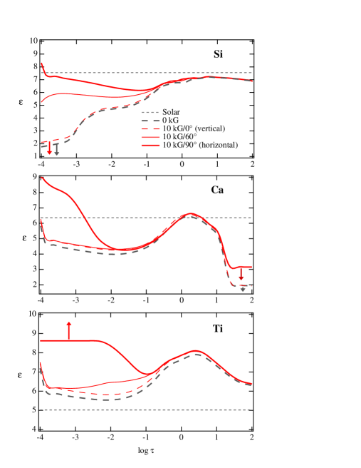
Figure 1: Abundance stratifications (equilibrium solutions) of Si, Ca, and Ti, for an atmosphere with $T_{\rm eff}=8\,500$ K and $\log\,g=4.0$. The logarithm of the abundance ($\varepsilon$) with respect to hydrogen (in units of $\log\,H=12$) is plotted against $\log\tau_{\rm 5000}$. The meaning of the different curves is given in the top panel (Si); the arrows indicate that the equilibrium solution is not reached in some layers and that equilibrium abundances should be smaller (or larger) than those displayed.

For layers higher than $\log\tau=-1.0$, the magnetic field is very efficient, especially when it is horizontal. This is generally due to the fact that element diffusion in the neutral state is favoured by the presence of a horizontal component of the magnetic field. Generally, the neutral state undergoes strong radiative acceleration (absorption lines are not saturated) and has a large diffusion coefficient. Silicon is still hardly supported in a horizontal field, but much better than in a vertical field. Calcium and titanium abundances are clearly enhanced above $\log\tau=-2.0$ for a horizontal field.

According to the surface abundance patterns reconstructed by Kochukhov et al. (koc04 (2004)) for 53 Cam (their Fig. 10), Si is more abundant in places where the magnetic field is nearly horizontal. This is consistent with the trend shown in Fig. 1, but our predicted absolute abundances of Si are at variance with the maps, being always smaller than the solar value. This could be due to the higher gravity in our model than found for 53 Cam. Calcium is strongly stratified in our computations, with an enhancement only in layers above $\log\tau=-3.0$ in the presence of a strong horizontal magnetic field, but the correlation with the magnetic map of 53 Cam is less clear than in the case of Si. The Ti abundance map appears to be more or less anti-correlated with the Ca distribution, except near the visible magnetic pole. This anti-correlation could possibly be related to the cloud of Ti we find for a horizontal field about $\log\tau=-2.0$ and the hole of Ca we find in the same layers. At the magnetic pole, both Ca and Ti are enhanced in 53 Cam. In Fig. 1, Ca and Ti equilibrium stratifications near the magnetic poles can be deduced from the dashed lines. One notices that both curves have very similar profiles, apart from their distance to the respective solar values. Does this similarity explain the enhancements of Ca and Ti at the visible pole of 53 Cam? One cannot make this assertion from our results. It could also be the signature of mass loss at the magnetic pole in combination with the diffusion velocity (see the discussion by Babel & Michaud, bam91 (1991)), and in that case, an equilibrium solution cannot account for this kind of situation.

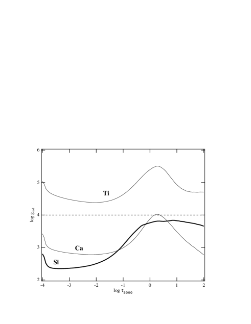
Figure 2: Radiative accelerations of Si, Ca, and Ti [$\log(cm\,s^{-2})$] for a zero magnetic field and solar homogeneous abundances in the atmospheric model of Fig. 1. The dashed line indicates the gravity.

4.3 Stratifications for $T_{\rm eff}=10\,000$ K

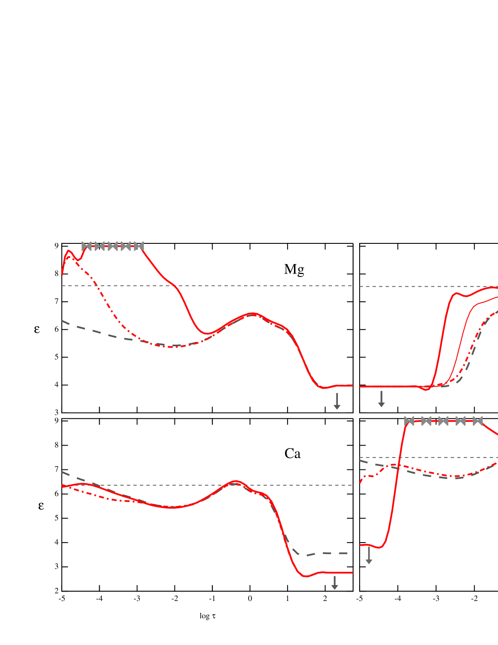
Figure 3: Abundance stratifications (equilibrium solutions) of Mg, Si, Ca, and Fe, for an atmosphere with $T_{\rm eff}=10\,000$ K. The dashed-point lines correspond to the case of a 1 kG horizontal magnetic field, for the other curves the legends are the same as in Fig. 1 (see text for details).

Equilibrium solutions for Mg, Si, Ca, and Fe are shown in Fig. 3. The effective temperature of $10\,000$ K is higher than the one adopted by Kochukhov et al. (koc06 (2006)) for HD 133792 ($9\,400\pm 200$ K), and the gravity of the model we used is also larger ($4.0$ instead of $3.7$). However, these values are close enough to allow a comparison of our results with the stratifications observationally deduced for this star.

For Mg, Ca, and Fe, the magnetic cases with angles 0 and 60 degrees are not shown because they cannot really be distinguished from the non-magnetic case. One notices that for Si and Ca, equilibrium solutions are clearly different from those found for $T_{\rm eff}=8\,500$ K; the same is true for radiative accelerations (compare Fig. 4 to Fig. 2). The plateau for Mg and Fe (in a 10 kG field) around $\log\tau=-3.0$ is due to the fact that we limit the abundances to $\varepsilon\leq 9.0$ . Larger abundances could be unphysical since our computations are done in the test-particle approximation and for an atmospheric model with solar abundance. For this particular model, we also considered the case of a moderate horizontal field strength of 1 kG (close to the average field observed in HD 133792). One can see that its effect is non-negligible for Mg. This is due to the strong contribution (enhanced by the horizontal magnetic field) of Mg i to the diffusion velocity.

We can compare these stratifications to those derived from high resolution spectra of HD 133792 by Kochukhov et al. (koc06 (2006)) and shown in their Fig. 5. For Mg, they find a strong accumulation (about 2 dex) above $\log\tau=-3.0$. Our equilibrium solution shows the same kind of enhancement for 1 kG, and a deficiency of Mg around $\log\tau=-2.0$. The contrast between overabundant layers and underabundant layers is also about $10^{2}$, but our equilibrium solution is more complex and predicts a Mg cloud that is more pronounced and goes deeper for a 10 kG horizontal field.

For Si, our equilibrium solution gives a decrease in the Si abundance above $\log\tau=0.5$ and a very strong depletion (3 dex) in layers higher than $\log\tau=-2.0$. Again, the contrast is comparable to what is deduced from observed spectra, but the drop in Si abundance occurs higher up in the atmosphere in our solution, the height of the drop increasing with the strength of the magnetic field.

For Ca, our equilibrium solution is quite different from the stratification proposed by Kochukhov et al. (koc06 (2006)), since the equilibrium solution shows a moderate decrease in the Ca abundance around $\log\tau=-2.0$ and not a step-function-like decrease like the one derived from the spectral analysis. On the other hand, Ca is strongly underabundant below $\log\tau=0.5$ in the equilibrium solution (as in the case of the $T_{\rm eff}=8\,500$ K model), because in these layers Ca is mainly in noble gas configuration (Ca III) for which the radiative acceleration is weak. We doubt that the spectral analysis used by Kochukhov et al. (koc06 (2006)) can reliably diagnose these optically thick deep layers.

For Fe, the equilibrium solution for a horizontal field of $<1$ kG reveals a contrast of about 1.5 dex between overabundant layers (around $\log\tau=0.0$) and deficient layers (above $\log\tau=-2.0$). This is of the same order of magnitude as what has been observationally derived for HD 133792. The transition between overabundant and deficient layers occurs more or less at the same depth in the empirical profile and in our equilibrium solution, but the stratification profile is not monotonic in the latter and does not exhibit, as the empirical profile does, a sharp drop above $\log\tau=-2.5$ from a strong enhancement below.

Figure 4: Radiative accelerations of Mg, Si, Ca, and Fe [$\log(cm.s^{-2})$] for zero magnetic field and solar homogeneous abundances in the atmospheric model of Fig. 3. The dashed line indicates the gravity.

4.4 Stratifications for $T_{\rm eff}=12\,000$ K

We also had a look at the behaviour of silicon in a hotter model, although we have not found corresponding recent observations with stratification analysis. This element is known to be enhanced in magnetic Ap stars but not in HgMn stars. According to Fig. 5, the equilibrium solution we have found is consistent with such observations. Silicon clearly appears to be deficient above $\log\tau=-1.0$ in the non-magnetic case. But, with a 10 kG horizontal magnetic field, a cloud of Si forms near $\log\tau=-2.0$, which should lead to an apparent overabundance. It is to be noted that, according to the accelerations shown in Fig. 6, a solar abundance of Si is not supported by the radiation field around $\log\tau=-2.0$, even for a 10 kG field! At first sight, this would appear to be at variance with the cloud found in Fig. 5. In fact, this is not so: due to the deficiency of Si around $\log\tau=-1.0$ (just below the cloud), more photons are available than in the solar case to support the Si cloud. This is a typical behaviour in the optically thin case, which cannot be encountered in stellar interiors.

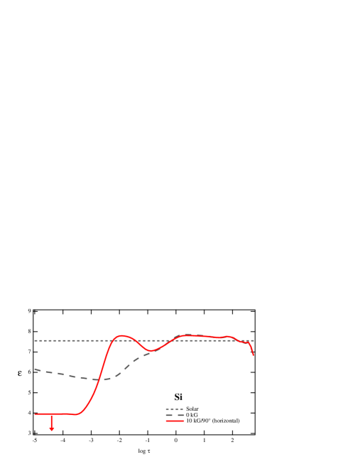
Figure 5: Abundance stratifications (equilibrium solutions) of Si, for an atmosphere with $T_{\rm eff}=12\,000$ K (same legend as Fig. 3). In the magnetic case, some layers around $\log\tau=-2.0$ could exhibit an overabundance of Si. However, according to the accelerations shown in Fig. 6 (long-dashed curve) Si is not supported above $\log\tau=0.0$ for solar abundance. The local overabundance is due to the deficiency of Si below these layers: the medium being optically thin, more photons come from deficient layers and support silicon in the layers above.

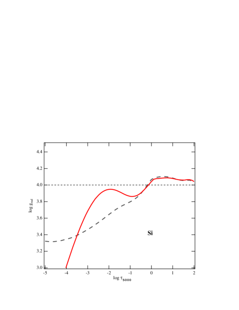
Figure 6: Radiative accelerations of Si [$\log(cm.s^{-2})$] for homogeneous solar abundance and the atmospheric model of Fig. 5. The dashed line indicates the gravity. The long-dashed curve is the acceleration for zero magnetic field, and the solid line is the total acceleration in the magnetic case (as defined in Alecian & Stift, als06 (2006), Eq. 13).

5 Conclusions

In this work we present the first detailed numerical calculations of element stratifications due to atomic diffusion in magnetic atmospheres. This study addresses the abundance anomalies observed in Ap stars, either magnetic or non-magnetic (HgMn stars). Radiative accelerations are based on full opacity sampling of Zeeman split spectral lines, and diffusion velocities are obtained by the methods described in Alecian & Stift (als06 (2006)). The stratifications derived in the present study correspond to equilibrium solutions: one looks for abundance stratifications such that diffusion velocities are close to zero everywhere in the atmosphere.

Because of the high computational cost, we restricted our study to a few metals and stellar atmospheres. We want to explore those cases where our results can be compared with observed abundance maps and stratifications. We did not try to use atmospheric models corresponding perfectly to those derived from the observations of 53 Cam and of HD 133792, but instead used standard solar abundance ATLAS9 models that are close enough to allow a meaningful discussion. It emerges from this comparison that, in several cases, equilibrium solutions are consistent with stratifications reconstructed from observed Stokes spectra by means of magnetic Doppler imaging. However, significant differences also exist. Some of these differences may be partly due to possible shortcomings in the inversion of the observational material, but one has to keep in mind that our modelling approach, with its search of equilibrium stratifications, is more likely to be responsible. Indeed, equilibrium solutions can be very different from the stratifications encountered in real stars, which result from non-linear, time-dependent processes, with a competition between several physical processes (atomic diffusion, inhomogeneous mass-loss, complex magnetic geometries, NLTE effects, turbulence, etc.). The present study constitutes one more step toward the detailed modelling of magnetic atmospheres, but for the first time in this quest, the results we obtain can be compared with observations. Time-dependent atomic diffusion is the next step, which we shall address in the near future.

- (1) Alecian, G., 1982, A&A, 107, 61
- (2) Alecian, G., & Grappin, R. 1984, A&A, 140, 159
- (3) Alecian, G., & Michaud, G. 1981, ApJ, 245, 226
- (4) Alecian, G., & Stift, M.J. 2004, A&A, 416, 703
- (5) Alecian, G., & Stift, M.J. 2006, A&A, 454, 571
- (6) Alecian, G., & Vauclair, S. 1981, A&A, 101, 16
- (7) Babel, J., 1992, A&A, 258, 449
- (8) Babel, J., & Michaud, G. 1991, ApJ, 366, 560
- (9) Bischof, K.M., 2005, Mem. Soc. Astron. Italiana, Suppl. 8, 64
- (10) Cunto, W., & Mendoza, C. 1992, Rev. Mex. Astron. Astrofis., 23, 107
- (11) Cunto, W., Mendoza, C., Ochsenbein, F., & Zeippen, C.J. 1993, A&A 275, L5
- Hui-Bon-Hoa et al. (2000) Hui-Bon-Hoa, A., LeBlanc, F. & Hauschildt, P. H. 2000, ApJ, 535, L43
- (13) Hui-Bon-Hoa, A., LeBlanc, F., Hauschildt, P.H., & Baron, E. 2002, A&A, 381, 197
- (14) Kochukhov, O., Bagnulo, S., Wade, G.A., Sangalli, L., Piskunov, N., Landstreet, J.D., Petit, P., & Sigut, T.A.A. 2004, A&A, 414, 613
- (15) Kochukhov, O., Tsymbal , V., Ryabchikova, T., Makaganyk, V., and Bagnulo, S. 2006, A&A, 460, 831.
- (16) Kurucz, R. 1993, CDROM Model Distribution, Smithsonian Astrophys. Obs.
- (17) Michaud, G. 1970, ApJ, 160, 641
- (18) Schatzman, E. 1969, A&A, 3, 331
- (19) Seaton, M.J., 1999, MNRAS, 307, 1008
- (20) Smith, K.C. & Dworetsky, M.M., 1993, A&A, 274, 335
- (21) Turcotte S., Richer J. & Michaud G., 1998, ApJ, 504, 559
- (22) Vauclair, S., Hardorp, J., & Peterson, D.M. 1979, ApJ, 227, 526