Numerical analysis of solitons profiles
in a composite model for DNA torsion dynamics

Abstract

We present the results of our numerical analysis of a “composite” model of DNA which generalizes a well-known elementary torsional model of Yakushevich by allowing bases to move independently from the backbone. The model shares with the Yakushevich model many features and results but it represents an improvement from both the conceptual and the phenomenological point of view. It provides a more realistic description of DNA and possibly a justification for the use of models which consider the DNA chain as uniform. It shows that the existence of solitons is a generic feature of the underlying nonlinear dynamics and is to a large extent independent of the detailed modelling of DNA. As opposite to the Yakushevich model, where it is needed to use an unphysical value for the torsion in order to induce the correct velocity of sound, the model we consider supports solitonic solutions, qualitatively and quantitatively very similar to the Yakushevich solitons, in a fully realistic range of all the physical parameters characterizing the DNA.

I Introduction

It is now almost thirty years that the role of solitons in fundamental DNA functions is under serious investigation (see Cadoni et al. (2007a, b) for a long list of references). In particular a lot of efforts have been made lately Roberts (1993); Huang and MacKerell (2004); Horton et al. (2004) to study the phenomenon of the so-called base-flipping, namely the complete opening of a narrow segment of DNA, a phenomenon which is thought to be important for fundamental processes such as replication and transcription.

A successful elementary model for DNA rotational modes, introduced by Yakushevich Yakushevich et al. (2002), makes use of a double chain of oscillators where every node of each chain is represented by a disc which interacts with their first neighbors on the same chain and with the disc in front of it on the other chain.

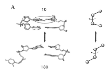
Figure 1: A picture (extracted from Banavali et al. (2002)) showing the phenomenon of base-flipping, namely the complete opening of a DNA’s base pair due to the rotation of (at least) on of them by an angle of $\pi$. It is clear from the picture that in the process of rotating about the DNA axis both the sugar and base planes also rotate about some other axis; to simplify as much as possible our model we will disregard this effect and concetrate only on the rotation about DNA’s axis.

The homogeneous version of this model succeds in supporting the existence of topological solitons for a wide range of the physical and geometrical parameters, also allowing analytical solutions for a few cases, but it was shown Yakushevich et al. (2002) that adding enough inhomogeneities – i.e. taking into account the geometrical and dynamical differences between the four possible bases for a realistic DNA segment – causes solitons to lose energy and finally stop their motion after a few nodes on the chain.

Our final goal, which will not be reached within this paper, is to determine whether or not realistic segments of DNA support the motion of “rotational” solitons. In the composite model proposed in Cadoni et al. (2007a), by separating the degrees of freedom of the bases from the backbone-sugar component, we produced a model where the component supporting the solitons, i.e. the backbone-sugar chain, is perfectly homogeneous and the bases inhomogeneities act just as a perturbation of a homogenous system, leaving hope for a longer life of solitons moving on it. We leave to a future paper the study of the profiles of solitons in inhomogeneous chains and their time evolution.

The numerical results we present in this paper support our guess that the composite model represents an important improvement of the simple torsional models for DNA dynamics in the homogeneous approximation: it supports the existence of solitons and moreover these solitons are very close to the corresponding ones in the Yakushevich model. As a bonus, the increase in the geometrical (and consequentely dynamical) detail turned out to be enough to allow the generation of the solitons corresponding to the Yakushevich ones using for the coupling constants values which are compatible with the physical ones .

As a final remark, we point out that all numerical results and estimates of the geometrical and dynamical parameters included in this paper are an improvement and/or an update of the corrisponding ones published in Cadoni et al. (2007a), which is fully superseded by this one.

II Model & equations

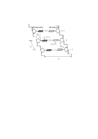
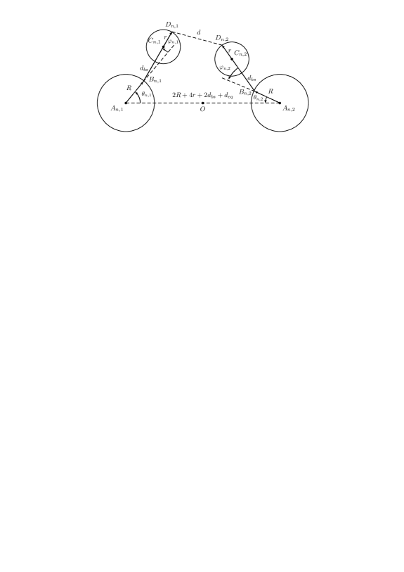
Figure 2: Left. A fragment of our “composite” model of the DNA’s double chain: at every node of the chain there are four degrees of freedom, two for each base (the $\{\varphi_{n,i}\}$) and two for each sugar-phosphate group (the $\{\theta_{n,i}\}$). Right. Detail of a chain node. Every base $\{n,i\}$ is allowed to rotate about the $C_{1}$ atom of the corresponding sugar (see fig. 3), represented by the point $B_{n,i}$, only by an angle between $[-\pi/2,\pi/2]$ because of the physical contraint represented by the sugar pentagon, so that the effective phase space of the model is $({\mathbb{S}}^{1}\times[-\pi/2,\pi/2])^{2n}$; this steric constraint is implemented in the model dynamically through an effective potential. See sec. III for an evaluation of all geometrical constants that appear in the pictures above.

Our model for DNA is a homogeneous double chain of coupled double pendula which is a natural generalization of a well known model by Yakushevich  where, at every node of each chain, the whole group base-sugar-phosphate is represented by a single disc centered at the chain’s backbone axis: we simply split the group in two distinct discs, one still centered about the backbone axis and representing the sugar-phosphate group and the second rigidly rotating about a fixed point of the former as shown in fig. 2 (note that, in order to keep the geometry of the model as simple as possible, we consider the chain as plane rather than helicoidal).

Referring to fig. 2, the coordinates of the two discs centers and of the extrema of bases, whose distance we use to determine the intensity of the bonds between the base pairs on the same chain node, are the following:

$$A_{n,i}$$

where $h=2R+4r+2d_{bs}+d_{eq}$.

The dynamical evolution of our mechanical system is determined by the Lagrangian $L=T-V$, where $T$ is the kinetic energy and $V$ is the interaction potential. The interactions that are relevant for DNA rotational dynamics are five:

1. The torsion ($V_{t}$) between next neighbor sugar-phosphate groups on the same chain, representing the torsional elasticity of the backbone. This force is the results of complex molecular interactions at the backbone level and it is to be considered an “effective” term. Following the principle of keeping the potential expressions as simple as possible until some good reason is found to make them more complicated and keeping in mind that $\theta$ can vary on the whole circle, we use for it the “physical pendulum” periodic potential

   $$V_{t}=\sum_{n=1}^{N-1}\sum_{i=1}^{2}K_{t}\left[1-\cos(\Delta\theta_{n,i})\right]$$ (II.1)

   where $\Delta\theta_{n,i}=\theta_{n+1,i}-\theta_{n,i}$. Note that relative angles between next neighbor discs never get big, so that it would be safe also to use its harmonic approximation $Vt\simeq\sum_{n=1}^{N-1}\sum_{i=1}^{2}K_{t}/2[\Delta\theta_{n,i}]^{2}$.

2. The stacking ($V_{s}$) between next neighbors bases on the same chain, representing the $\pi-\pi$ bonds between the rings that constitute the bases. This interaction is much better understood than the previous one and in particular it is clear that only depends on the relative displacement between next neighbor bases, going rapidly to zero together with the overlapping portion of their surface, e.g. like in a Morse-like potential. However, since also in this case the relative angle of any two bases next to each other keeps small, we simplified its expression by considering it a harmonic bond depending on the “$xy$” distance between the centers of the bases:

   $$V_{s} =\displaystyle\sum_{n=1}^{N-1}\sum_{i=1}^{2}\frac{1}{2}K_{s}\;d^{2}_{xy}(C_{n+1,i},C_{n,i})$$ (II.4)

   $$=\displaystyle\sum_{n=1}^{N-1}\sum_{i=1}^{2}\frac{1}{2}K_{s}(d_{bs}+r)^{2}\bigg{\{}\left[\alpha(\cos\theta_{n+1,i}-\cos\theta_{n,i})+\cos(\theta_{n+1,i}+\varphi_{n+1,i})-\cos(\theta_{n,i}+\varphi_{n,i})\right]^{2}+$$

   $$\phantom{=\displaystyle\sum_{n=1}^{N-1}\sum_{i=1}^{2}\frac{1}{2}K_{s}(d_{bs}+r)^{2}\bigg{\{}[}\left[\alpha(\sin\theta_{n+1,i}-\sin\theta_{n,i})+\sin(\theta_{n+1,i}+\varphi_{n+1,i})-\sin(\theta_{n,i}+\varphi_{n,i})\right]^{2}\bigg{\}}$$

   where $\alpha=R/(d_{bs}+r)$.

3. The pairing ($V_{p}$) between bases on opposite chains, representing the ionic bonds which keep the helices together. This is the best understood force among the ones we are considering and, like in the stacking case, it is known to go rapidly to zero a few Angstrom far from the equilibrium position; in this case though the distance between pairs of bases does get big when a base is flipping and therefore a harmonic approximation result rather unphysical. The interaction can be more realistically modelled by a Morse-like potential Gaeta (2007), nevertheless we will produce profiles also in the harmonic approximation in order to compare our results with those in Yakushevich et al. (2002), so we will consider both cases:

   $$V_{p} =\displaystyle\sum_{n=1}^{N}D\left[1-e^{-\mu\;d(D_{n,1},D_{n,2}})\right]^{2}$$ (II.7)

   $$\simeq\displaystyle\sum_{n=1}^{N}\frac{1}{2}K_{p}(d_{bs}+2r)^{2}\bigg{\{}\left[\beta(\cos\theta_{n,1}+\cos\theta_{n,2})+\cos(\theta_{n,1}+\varphi_{n,1})+\cos(\theta_{n,2}+\varphi_{n,2})-2-2\beta\right]^{2}+$$

   $$\phantom{=\displaystyle\sum_{n=1}^{N}\frac{1}{2}K_{p}(d_{bs}+2r)^{2}\bigg{\{}[}\left[\beta(\sin\theta_{n,1}+\sin\theta_{n,2})+\sin(\theta_{n,1}+\varphi_{n,1})+\sin(\theta_{n,2}+\varphi_{n,2})\right]^{2}\bigg{\}}$$

   where $\beta=R/(d_{bs}+2r)$ and $K_{p}=2D\mu^{2}$ (see eq. (III.1)). Note that, in order to simplify the expression of the elongation from the equilibrium position, we made the “contact” approximation $d_{eq}=0$, i.e. we disregarded the inter-bases distance in the equilibrium position; we will show numerically in sec. IV that this does not change significantly the solitons profiles. The same is knonw to hold also in the Yakushevich model.

4. The helicoidal interactions ($V_{h}$) between nucleotides, which are mediated by water filaments (Bernal-Fowler filaments). This is the only ingredient of our model which is reminiscent of the helicoidal structure of DNA; in particular we will consider those being on opposite helices at half-pitch distance, as they are near enough in three-dimensional space due to the double helical geometry. As the nucleotide move, the hydrogen bonds in these filaments – and those connecting the filaments to the nucleotides – are stretched and thus resist differential motions of the two connected nucleotides. We will, for the sake of simplicity and also in view of the small energies involved, only consider filaments forming between the sugar-phosphate groups, thus only the backbone angles will be involved in these interactions. Recalling that the pitch of the helix corresponds to 10 bases in the B-DNA equilibrium configuration we set

   $$V_{h}=\sum_{n=1}^{N}\sum_{i=1}^{2}K_{h}\left[1-\cos(\theta_{n+5,i+1}-\theta_{n,i})\right]$$ (II.8)

   where the sum $i+1$ is meant modulo 2.

5. The sugar wall ($V_{sw}$), representing an “effective” interaction which dynamically restricts the range of the base angles $\varphi_{n,i}$ to some interval $[\varphi_{-},\varphi_{+}]$ – ruling out this way the possibility of topologically non trivial configurations for them – to represent the steric constraint represented by the sugars, which prevents the corresponding bases from doing a complete circle about them. We set these angles to $\phi_{\pm}=\pm\pi/2$ and verified numerically that the profiles in the composite model converge to the corresponding ones by narrowing more and more the interval $[\varphi_{-},\varphi_{+}]$. In order not to interfere with the dynamics close to the equilibria positions the potential must be as flat as possible close to the zeroes of the $\varphi_{n,i}$ and must rise rather quickly when the $\varphi_{n,i}$ approach $\pm\pi/2$. A natural choice, which we implemented in Cadoni et al. (2007a), would be to use some high power of the tangent function but divergences cause problem in numerical calculations so we use in this paper some high even power of the sine function.

   $$V_{sw}=\sum_{n=1}^{N}\sum_{i=1}^{2}K_{sw}\sin^{k}(\varphi_{n,i})$$ (II.9)

   where the coupling constant $K_{sw}$ must be taken big enough to prevent the bases from passing through the $\pm\pi/2$ barrier but also not so big to interfere too much with the dynamics when the $\varphi_{n,i}$ are closer to the equilibrium position.

As for the kynetic energy, a straightforward calculation shows that for the sugar-phosphate group we have

$$T_{t}=\sum_{n=1}^{N}\sum_{i=1}^{2}\frac{1}{2}I_{t}\dot{\theta}^{2}_{n,i}$$ (II.10)

and for the bases

$$T_{s}=\sum_{n=1}^{N}\sum_{i=1}^{2}\frac{1}{2}I_{s}\left[\dot{\varphi}^{2}_{n,i}+2(1+\alpha\cos\varphi_{n,i})\dot{\varphi}_{n,i}\dot{\theta}_{n,i}+(1+2\alpha\cos\varphi_{n,i}+\alpha^{2})\dot{\theta}^{2}_{n,i}\right]$$ (II.11)

Note that by putting the bases angles identically equal to zero the Lagrangian $L=T_{t}+T_{s}-V_{t}-V_{s}-V_{p}-V_{h}-V_{sw}$ of the composite model reduces, modulo the helicoidal term, exactly to the Yakushevich homogeneous Lagrangian:

$$L(\theta_{n,i},0,\dot{\theta}_{n,i},0)= \phantom{+}\displaystyle\sum_{n=1}^{N}\sum_{i=1}^{2}\frac{1}{2}\left[I_{t}+(1+\alpha)^{2}I_{s}\right]\dot{\theta}^{2}_{n,i}+\displaystyle\sum_{n=1}^{N-1}\sum_{i=1}^{2}\left[K_{t}+(1+\alpha)^{2}(d_{bs}+r)^{2}K_{s}\right]\left[1-\cos(\Delta\theta_{n,i})\right]$$ (II.12)

$$+\displaystyle\sum_{n=1}^{N}(1+\beta)^{2}(d_{bs}+2r)^{2}K_{p}\left\{2(1-\cos\theta_{n,1})+2(1-\cos\theta_{n,2})-\left[1-\cos(\theta_{n,1}-\theta_{n,2})\right]\right\}$$ (II.13)

Now, once an initial condition for all angles is given, the Lagrangian determines completely the evolution of the state as the “trajectory” $q(t)=(\theta_{n,i}(t),\varphi_{n,i}(t))$ extremizing the action $I=\int_{q(t)}L(q(t),\dot{q}(t))dt$. The initial states we are interested in are those ones which give rise to motions which do not change (much) shape, i.e. which move “rigidly”, satisfying therefore the “discrete wave” condition $q_{n+k,i}(t)=q_{n,i}(t-k\delta/v)$, where $\delta$ is the distance between two consecutive nodes. We look at these solutions as “discrete solitons” able to move on the DNA chain.

For a discussion about the analytical properties of the model we refer the reader to the paper Cadoni et al. (2007b). Even in the simplest cases it is impossible to find an explicit solution to the Lagrange equations and therefore the system must be analyzed numerically. To this end we use the fact that in our case $h=-\delta/v$ is small enough to claim that

$$\dot{q}_{n,i}(t)\simeq\frac{q_{n}(t-h)-q_{n}(t)}{-h}=-\frac{v}{\delta}[q_{n}(t+\delta/v)-q_{n}(t)]=-\frac{v}{\delta}\Delta_{n,i}[q(t)]$$

so that the kynetic energy becomes

$$T_{t}=\sum_{n=1}^{N}\sum_{i=1}^{2}\frac{I_{t}v^{2}}{2\delta^{2}}[\Delta\theta_{n,i}]^{2}$$

$$T_{s}=\sum_{n=1}^{N}\sum_{i=1}^{2}\frac{I_{s}v^{2}}{2\delta^{2}}\left\{[\Delta\varphi_{n,i}]^{2}+2(1+\alpha\cos\varphi_{n,i})\Delta\varphi_{n,i}\Delta\theta_{n,i}+(1+2\alpha\cos\varphi_{n,i}+\alpha^{2})[\Delta\theta_{n,i}]^{2}\right\}$$

Having discretized time we are left with just one degree of freedom, the discrete space coordinate $n$, so that what was previously the system lagrangian $L=\sum_{n=1}^{N}\sum_{i=1}^{2}L_{n,i}$ has become now the action (summed over $n$) of the discrete Lagrangian $L_{n}=\sum_{i=1}^{2}L_{n,i}$; the discrete Lagrange equations, by the minimum action principle, are clearly given simply by $dL=(\partial_{\theta_{n,i}}L,\partial_{\varphi_{n,i}}L,)=0$ and its solutions, subjected to opportune initial conditions, are exactly the profiles of the solitons that we want to make sure to be present in this generalization of the Yakushevich  model.

III Physical values of parameters & dispersion relations

The evaluation of the main geometrical and dynamical physical quantities entering in our model is far from being a trivial matter. There are still very few direct measurements, for example, of the stacking energy between bases within DNA and the torsional backbone force – due to quite complex interactions between the sugar and the phosphate atoms – is just an effective term for which it is hard in principle to define a strenght. Also for geometrical parameters things are not better and often in the literature different values for the same physical quantities are used. In this section we are going to give an estimate for the values of the parameters of our model.

III.1 Kinematical parameters

The kinematical parameters include the geometrical parameters, the mass $m$ and the momenta of inertia $I$. We opted to directly estimate them starting from PDB data PDB (note, as already mentioned, that the present results supersede the ones we used in Cadoni et al. (2007a))

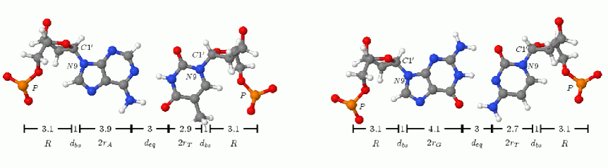
Figure 3: A node of the DNA chain with a AT pair (left) and a GC pair (right). The measures of the distances are meant as the projections of the actual lenghts over the axis connecting the two phosphates of the same chain node. The distance between the two phosphates is $h=18$Å for both base pairs.

The masses can be easily calculated on the basis of the chemical structure of DNA. Estimate of momenta of inertia is more involved, especially for the sugar-phosphate group, since the evaluation depends on the choice of the rotation axis and, as pointed out earlier, base-flipping rotations are a complex subject. In our evaluations we made the simplest approximation, namely momenta of inertia of sugar rings have been calculated with respect to rotations about the main axis of DNA and passing by $P$ atom of the backbone (see fig. 3) and inertia momenta of bases have been calculated with respect to rotations about the same axis by $C_{1}$ atom of the sugar ring.

The geometrical parameters of interest for our model are the longitudinal width of bases $l_{b}$ and of the sugar $l_{s}$, the distances of the bases from the relative sugars $d_{bs}$ and the distance of a base from the relative dual base $d_{eq}$. We give our estimates for the masses, moments of inertia and the geometrical parameters for the different bases and their mean values in table 1. From those data and using the notations $R=l_{s}$, $r={\bar{l}}_{d}/2$, $h=l_{s}+d_{bs}+{\bar{l}}_{b}+d_{eq}/2$, $h_{c}=l_{s}+d_{bs}+{\bar{l}}_{b}$ (the bar denotes the mean value), we get the average values for the geometrical parameters appearing in our Lagrangian shown in table 2.

	A	T	G	C	mean	Sugar
$m$	134	125	150	110	130	85
$I$	$3.6\times 10^{3}$	$3.0\times 10^{3}$	$4.4\times 10^{3}$	$2.3\times 10^{3}$	$3.3\times 10^{3}$	$2.9\times 10^{3}$
$l$	$3.9$	$2.9$	$4.1$	$2.7$	$3.4$	$3.1$
$d_{bs}$	$1.0$	$1.0$	$1.0$	$1.0$	$1.0$	-
$d_{eq}$	$3.0$	$3.0$	$3.0$	$3.0$	$3.0$	-

Table 1: Order of magnitude for the basic geometrical parameters of the DNA. Units of measure are: atomic unit for masses $m$, $1.67\times 10^{-47}{\rm Kg}\cdot{\rm m}^{2}$ for the inertia momenta $I$, Angstrom for $l$ (the longitudinal width of bases and sugar), $d_{bs}$ (the distances sugar-base) and $d_{eq}$ (the distance at the equilibrium for the pairs AT and GC). These values have been extracted from the sample “generic” B-DNA PDB data PDB , provided by the Glactone Project Gla , and double checked with the data from Drew et al. (1981), that agrees within $5\%$. As shown in fig. 3, the lengths of bases and sugar were taken by projecting them on the direction passing through the two phosphate atoms of the chain node to best fit the geometry of the model; the (real) measure for the diameters of the bases A, T, G, C, and the sugar and for $d_{bs}$ are respectively (in Å): 4.6, 4.0, 5.7, 4.0, 3.3 and 1.5.)

$R$	$r$	$d_{bs}$	$d_{eq}$	$h$	$h_{c}$	$\alpha$	$\beta$
3.1	1.7	1.0	3.0	18	15	1.1	0.7

Table 2: Numerical values (in Å) of the geometrical parameters characterizing our model. Here $h=2R+4r+2d_{bs}+d_{eq}$ is the width of DNA and $h_{c}=h|_{d_{0}=0}$ is its value in the contact approximation.

III.2 Dynamical parameters

The determination of the four coupling constants ($K_{p}$, $K_{t}$, $K_{s}$ and $K_{h}$) characterizing our model requires some assessments. Their order of magnitude can be estimated by considering the typical energies of hydrogen bonds ($K_{p}$) and the experimental results for the torsional rigidity of the chain ($K_{t}$ and $K_{s}$). As we will show later, the geometry of our composite model allows – with values for coupling constants within the experimental ranges – to make predictions about dynamical properties of DNA, as the induced optical frequencies and the phonon velocities, of the same order of magnitude of those experimetally observed (conversely, dispersion relations allow to restrict the selection of the coupling constants to those values which fit better our model).

III.2.1 Pairing

The coupling constant $K_{p}$ of the pairing potential (II.7) can be determined by considering the typical energy of hydrogen bonds. The pairing interaction involves two (in the $A-T$ case) or three (in the $G-C$ case) ionic hydrogen bonds. We can model the pairing potential with a Morse function like

$$V_{p}(d)=D[1-e^{-\mu(d-d_{eq})}]^{2}=\frac{1}{2}K_{p}(d-d_{eq})^{2}+O(d^{3})\,,$$ (III.1)

where $D$ is the potential depth, $d$ the distance between the points $D_{n,1}$ and $D_{n,2}$ (see fig. 2), $d_{eq}$ the bond equilibrium distance and $\mu$ a parameter that controls the width of the well.

Figure 4: Comparison of Morse potential and its correspondig harmonic approximation

Different estimates of the parameters appearing in the potential (III.1) are present in the literature. The estimates

$$D_{AT}=0.030\,{\hbox{eV}},\ D_{GC}=0.045\,{\hbox{eV}},\ \mu_{AT}=1.9\,{\rm\AA}^{-1},\ \mu_{GC}=2.5\,{\rm\AA}^{-1}$$

are given in Chen and Prohofsky (1992) and used in Zhang and Collins (1995). The values

$$D=0.040\,{\hbox{eV}},\ \mu=4.45\,{\rm\AA}^{-1}$$

are given in Peyrard et al. (1992) and used in Peyrard et al. (1992); Barbi et al. (1999); Luca et al. (2004). Finally, the estimates

$$D_{AT}=0.050\,{\hbox{eV}},\ D_{GC}=0.075\,{\hbox{eV}},\ \mu_{AT}=\mu_{GC}=4\,{\rm\AA}^{-1}$$

are given in Campa (2000) and used in Campa (2000); Komarova and Soffer (2005). The values of coupling constants corresponding to these different values for the parameters appearing in the Morse potential range across an order of magnitude:

$$3.5\,{\hbox{N/m}}\ \leq\ K_{p}\,:=\,2D\mu^{2}\ \leq\ 38\,{\hbox{N/m}}\ .$$ (III.2)

In our numerical investigations we will use a value of $K_{p}$ near to the lower bound given in (III.2); that is, we adopt the value $K_{p}=4\,{\hbox{N/m}}$ – corresponding to $D=0.030\,{\hbox{eV}},\ \mu=2\,{\rm\AA}^{-1}$ – which leads to an optical excitation threshold of $q_{4}=\sqrt{2K_{p}/m_{b}}\simeq 32\,{\rm cm}^{-1}$ (see eq. (III.18)), so to be in agreement with Powell et al. (1987).

III.2.2 Stacking

The determination of the torsion and stacking coupling constants is more challenging and is based on a smaller amount of experimental data. The main information is the total torsional rigidity of the DNA chain $C=S\delta$, where $\delta=3.4{\rm\AA}$ is the base-pair spacing and $S$ is the torsional rigidity. It is known Barkley and Zimm (1979); Bruant et al. (1999) that

$$10^{-28}\,{\rm J\cdot m}\ \leq\ C\ \leq 4\cdot 10^{-28}\,{\rm J}\cdot{\rm m}\ .$$ (III.3)

This information is used e.g. in Englander et al. (1980); Zhang (1989), whose estimate is based on the evaluation of the free energy of superhelical winding; this fixes the range for the total torsional energy to be

$$180\,{\hbox{kJ/mol}}\ \leq\ S\ \leq\ 720\,{\hbox{kJ/mol}}\ .$$ (III.4)

In our composite model the total torsional energy of the DNA chain has to be considered as the sum of two parts, the base stacking energy and the torsional energy of the sugar-phosphate backbone. In order to extract the stacking coupling constant we use the further information that $\pi-\pi$ stacking bonds amount at the most to $50{\hbox{kJ/mol}}$ Hunter and Sanders (1990); Khairoutdinov . The stacking potential can be described by a Morse potential whose width $\sigma$ is of the order 1Å – so that (see eq. (II.4)) the harmonic approximation is justified – and assuming for the stacking energy the highest value possible, the coupling constant value is $K_{s}=2E_{s}/\sigma^{2}\simeq 16.6{\hbox{N/m}}$. The phonon speed induced by this value of $K_{s}$ is $c_{3}=\delta\sqrt{K_{s}/m_{b}}\simeq 3{\hbox{km/s}}$ (see eq. (III.18)), which is rather close to the the estimate of $1.8{\hbox{km/s}}\leq c_{1}\leq 3.5{\hbox{km/s}}$ given in Yakushevich et al. (2002).

III.2.3 Torsion and helicoidal couplings

Once picked up the stacking component, our estimate for the torsional coupling constant $K_{t}$ falls in the range

$$130\,{\hbox{kJ/mol}}\ \leq\ K_{t}\ \leq\ 670\,{\hbox{kJ/mol}}\ .$$ (III.5)

Assuming (see Gaeta (1999)) that $K_{h}\simeq K_{t}/25=5\,{\hbox{kJ/mol}}$, so that $c_{4}=\sqrt{2K_{t}/I_{s}}$ (see equations (III.18) and (III.19)), all of these values for $K_{t}$ induce phonon speeds slightly higher with respect to the estimates cited above, between 5 km/s and 11 km/s. For our numerical investigations, to keep the phonon speed as low as possible, we will set $K_{t}=130\,{\hbox{kJ/mol}}$.

III.2.4 Sugar wall

In order to have a barrier flat enough close to the equilibrium position we chose to use the exponent $k=100$ in II.9. Numerical tests show that a value of at least $K_{sw}=10^{4}\,{\hbox{kJ/mol}}$ is needed in order to keep the bases angles within the $[-\pi/2,\pi/2]$ interval.

$K_{t}$	$K_{s}$	$K_{p}$	$K_{h}$	$K_{sw}$
130 kJ/mol	16.6 N/m	3.5 N/m	5 kJ/mol	$2\cdot 10^{4}$ kJ/mol
$g_{t}$	$g_{s}$	$g_{p}$	$g_{h}$	$g_{sw}$
0.58	1.62	1	0.02	100

Table 3: Values of the coupling constants (above) and of their normalized counterpart (below).

For numerical calculations it is more convenient to renormalize the Lagrangian with respect to some energy value in order to work with dimensionless quantities. To be coherent with the Yakushevich work we renormalized the Lagrangian with respect to the pairing coefficient $l_{p}=K_{p}(d_{bs}+2r)^{2}/2\simeq 223\,{\hbox{kJ/mol}}$; the values of renormalized coefficients for coupling constants $g_{t}=K_{t}/l_{p}$, $g_{s}=K_{s}(d_{bs}+r)^{2}/2/l_{p}$, $g_{h}=K_{h}/l_{p}$ and $g_{sw}=K_{sw}/l_{p}$ are summarized in table 3.

Comparing equation II.12 with the potential used by Yakushevich in Yakushevich et al. (2002) it is easy to see that the coupling constant values induced on the Yakushevich model are given by

$$g=2g_{t}+4(1+\alpha)^{2}g_{s}\simeq 30\;,\;\;K=2(1+\beta)^{2}g_{p}\simeq 5.8$$ (III.6)

so that the normalized Yakushevich coupling constant (the torsional one) corresponding to our choice of parameters is $g/K\simeq 5.1$.

Note that, when using the Morse expression for pairing, the constant in front of the pairing is simply the bond energy $D=0.1\,{\hbox{kJ/mol}}$ (see eq. (II.7)). We decide nevertheless to divide by the same normalizing factor $l_{p}=K_{p}(d_{bs}+2r)^{2}/2=D\mu^{2}$ so that all dimensionless coupling constants are unchanged except for the pairing one which becomes $g_{p}^{\prime}=1/\mu^{2}\simeq 0.013$.

III.3 Dispersion relations

The linearized version of the composite Lagrangian is

$$L_{\hbox{lin}}(\theta_{n,i},\varphi_{n,i},\dot{\theta}_{n,i},\dot{\varphi}_{n,i})= \phantom{+}\displaystyle\sum_{n=1}^{N}\sum_{i=1}^{2}\left\{\frac{1}{2}I_{t}\dot{\theta}^{2}_{n,i}+\frac{1}{2}I_{s}\left[\dot{\varphi}_{n,i}+(1+\alpha)\dot{\theta}_{n,i}\right]^{2}\right\}$$ (III.11)

$$-\displaystyle\sum_{n=1}^{N-1}\sum_{i=1}^{2}\frac{1}{2}K_{t}\left[\Delta\theta_{n,i}\right]^{2}$$

$$-\displaystyle\sum_{n=1}^{N-1}\sum_{i=1}^{2}\frac{1}{2}K_{s}(d_{bs}+r)^{2}\left[\Delta\varphi_{n,i}+(1+\alpha)\Delta\theta_{n,i}\right]^{2}$$

$$-\displaystyle\sum_{n=1}^{N}\frac{1}{2}K_{p}(d_{bs}+2r)^{2}\left[\varphi_{n,1}+\varphi_{n,2}+(1+\beta)(\theta_{n,1}+\theta_{n,2})\right]^{2}$$

$$-\displaystyle\sum_{n=1}^{N}\sum_{i=1}^{2}\frac{1}{2}K_{h}[\theta_{n+5,i+1}-\theta_{n,i}]^{2}$$

leading to the following equations of motion:

$$\begin{cases}I_{t}\ddot{\theta}_{n,i}+(1+\alpha)I_{s}[\ddot{\varphi}_{n,i}+(1+\alpha)\ddot{\theta}_{n,i}]=&-K_{t}\square\theta_{n,i}\cr&-K_{s}(d_{bs}+r)^{2}(1+\alpha)[\square\varphi_{n,i}+(1+\alpha)\square\theta_{n,i}]\cr&-K_{p}(d_{bs}+2r)^{2}(1+\beta)\left[\varphi_{n,1}+\varphi_{n,2}+(1+\beta)(\theta_{n,1}+\theta_{n,2})\right]\cr&-K_{h}\left[-\theta_{n+5,i+1}+2\theta_{n,i}-\theta_{n-5,i+1}\right]\cr I_{s}[\ddot{\varphi}_{n,i}+(1+\alpha)\ddot{\theta}_{n,i}]=&-K_{s}(d_{bs}+r)^{2}[\square\varphi_{n,i}+(1+\alpha)\square\theta_{n,i}]\cr&-K_{p}(d_{bs}+2r)^{2}\left[\varphi_{n,1}+\varphi_{n,2}+(1+\beta)(\theta_{n,1}+\theta_{n,2})\right]\cr\end{cases}$$ (III.12)

where $\square\theta_{n,i}=-\theta_{n+1,i}+2\theta_{n,i}-\theta_{n-1,i}$ and similarly for $\varphi$. What we are interested in are the conditions for the existence of wave solutions for the equations above, i.e. in the form

$$\theta_{n,j}=\Theta_{\omega,k,j}\,e^{i(k\delta n+\omega t)}\;,\;\;\varphi_{n,j}=\Phi_{\omega,k,j}\,e^{i(k\delta n+\omega t)}\;,\;\;j=1,2$$

In the approximation $\alpha\simeq\beta$, namely considering the bases as pointlike, it is easy to simplify a pair of equations by multiplying the second equation by $(1+\alpha)$ and substracting it from the first one so that we are left with the pair

$$I_{t}\ddot{\theta}_{n,i}=-K_{t}\square\theta_{n,i}-K_{h}\left[-\theta_{n+5,i+1}+2\theta_{n,i}-\theta_{n-5,i+1}\right]\;,\;\;i=1,2$$

Summing and subtracting and imposing the wave form for the angles on the two equations above we find, by imposing the condition for the existence of non-trivial waves, the first pair of dispersion relations:

$$\omega_{1}^{2} = 4(K_{t}/I_{t})\sin^{2}(k\delta/2)+2(K_{h}/I_{t})[1+\cos(5k\delta)]$$ (III.13)

$$\omega_{2}^{2} = 4(K_{t}/I_{t})\sin^{2}(k\delta/2)+4(K_{h}/I_{t})\sin^{2}(5k\delta/2)$$ (III.14)

The second pair of the dispersion relations can then be easily extracted from the remaining pair of equations after the change of coordinates $\psi_{n,i}=\varphi_{n,i}+(1+\alpha)\theta_{n,i}$, the approximation $d_{bs}+2r\simeq d_{bs}+r$ (which in turn implies $\alpha=\beta$) and finally the fact that $I_{s}/(d_{bs}+r)^{2}$ is the mass $m_{b}$ of the base; the pair of equations then become

$$\begin{cases}m_{b}\ddot{\psi}_{n,1}=&-K_{s}\square\psi_{n,1}-K_{p}\left[\psi_{n,1}+\psi_{n,2}\right]\cr m_{b}\ddot{\psi}_{n,2}=&-K_{s}\square\psi_{n,2}-K_{p}\left[\psi_{n,1}+\psi_{n,2}\right]\cr\end{cases}$$

Restricting the equations on the wave solutions and summing and subtracting them we find the other pair of dispersion relations

$$\omega_{3}^{2} = 4(K_{s}/m_{b})\sin^{2}(k\delta/2)$$ (III.15)

$$\omega_{4}^{2} = 4(K_{s}/m_{b})\sin^{2}(k\delta/2)+2K_{p}/m_{b}$$ (III.16)

Physically, the four dispersion relations correspond to the four oscillation modes of the system in the linear regime. The relations involving $\omega_{1}$ and $\omega_{2}$ are associated with torsional oscillations of the backbone. In case of $\omega_{1}$ there is a threshold for the generation of the excitation originating in the helicoidal interaction, whereas the second torsional mode $\omega_{2}$ has no threshold and is thus also of acoustical type. The relation involving $\omega_{3}$ describes relative oscillations of the two bases in the chain with respect to the neighboring bases. As $\omega_{3}(k)\to 0$ for $k\to 0$ there is no threshold for the generation of these phonon mode excitations. The dispersion relation involving $\omega_{4}$ describes relative oscillations of two bases in a pair. The threshold for the generation of the excitation is now determined by the pairing interaction.

The dispersion relations (III.13,III.15) for values of the physical parameters given in the tables 1 and 3 are plotted in Fig. 5; there we plot $\omega/(2\pi c)$, where $c$ is the speed of light (we use the, in the literature widespread, convention of measuring frequencies in $2\pi c$ units) versus $k\delta/2$.

The four dispersion relations take a simple form if we consider excitations with wavelength $\lambda$ much bigger then the intrapair distance, i.e $\lambda\gg\delta$; this corresponds to the $\delta\to 0$ limit. We have then

$$\omega^{2}_{\alpha}\,-\,c^{2}_{\alpha}\,k^{2}\ =\ q^{2}_{\alpha}\ ,$$ (III.17)

where $c_{\alpha}$ and $q_{\alpha}$ ($\alpha=1\ldots 4$) are, respectively, the velocity of propagation (in the limit $k\gg q_{\alpha}$) and the excitation threshold. They are given by

$$\begin{array}[]{ll}c_{1}=\delta\sqrt{(K_{t}-25K_{h})/I_{t}},&q_{1}=2\sqrt{K_{h}/I_{t}};\\ c_{2}=\delta\sqrt{(K_{t}+25K_{h})/I_{t}},&q_{2}=0;\\ c_{3}=\delta\sqrt{K_{s}/m_{b}},&q_{3}=0;\\ c_{4}=\delta\sqrt{K_{s}/m_{b}},&q_{4}=\sqrt{2K_{p}/m_{b}};\\ \end{array}$$ (III.18)

Using the values of the parameters given in the tables 1 and 3 we have

$$\begin{array}[]{ll}c_{1}\simeq 0\,{\hbox{km/s}},&q_{1}\simeq 4.5\,{\rm{cm}^{-1}}\ ;\\ c_{2}\simeq 1\,{\hbox{km/s}},&q_{2}=0\ ;\\ c_{3}\simeq 3\,{\hbox{km/s}},&q_{3}=0\ ;\\ c_{4}\simeq 3\,{\hbox{km/s}},&q_{4}\simeq 32\,{\rm{cm}}^{-1}\ ,\\ \end{array}$$ (III.19)

where $c_{1}\simeq 0$ comes from the fact that we are taking $K_{t}\simeq 25\,K_{h}$ (see table 3 – this of course just means that $c_{1}$ is at least an order of magnitude smaller than the other $c_{i}$, and therefore negligible). Speeds can be converted to base per seconds by dividing each $c_{i}$ by $\delta=3.4$Å; excitation thresholds can be converted in inverse of seconds by multiplying each $q_{i}$ by $2\pi c$, where $c$ is the speed of light.

Figure 5: Graph of the dispersion relations (III.13,III.15) in the first Brillouin zone. We plot $\omega_{\alpha}/(2\pi c)$ ($c$ is the speed of light) as a function of $k\delta/2$. The $\omega_{1},\omega_{2},\omega_{3},\omega_{4}$ are represented respectively by the thick continuous, thin dashed, thin continuous and thick dashed line. Units are $\rm{cm^{-1}}$ in the vertical axis and radiants in the horizontal axis.

IV Numerical analysis

As we pointed out in sec. II, the profiles of the solitons in our model are extremals of the function of $4N$ variables $L(\theta_{n,i},\varphi_{n,i})$, where $N$ is the number of nodes of the chain. The interval of variations of the Lagrangian parameters under our study is such that solitons can have a radius of more than a hundred nodes so a reasonable value of $N$ is of the order of $10^{3}$; following Yakushevich Yakushevich et al. (2002) we mostly used the value $N=2000$.

Clearly the extremals – which by the way in our case turn out to be always maxima – of such a complex function of so many variables can only be obtained numerically; to accomplish that, again following Yakushevich, we choose to use the so-called conjugate gradients method. Ready-to-use implementations of this algorithm are available in the main numerical libraries, in particular in Numerical Recipes (NR, NR ) and in the GNU Scientific Library (GSL,  GSL ). As a double check, most of the results presented here have been produced using both implementations; all profiles shown in this paper were produced with GSL.

IV.1 Solitons profiles in the Yakushevich model

As a generalization of the sine-Gordon solitons, also the Yakushevich solitons are “relativistic” and in particular admit a limit speed beyond which no solution exists. We verified numerically that, for a fixed choice of the coupling constants, solitons profiles corresponding to all possible speeds vary by less than $10\%$ from each other, so that it is enough to show the profiles for a single value of the speed. All profiles presented here are relative to static solitons – in other words non-trivial equilibria position of the double chain; in this case the kynetic term is zero and the only parameter left in the renormalized Lagrangian is the coupling constant $g$ of the torsion potential.

As starting point for the extremizing algorithm, following Yakushevich, we used

$$\theta_{n,i}=q_{i}\pi\left\{1+\tanh\left[M(2n-N)\right]\right\}$$ (IV.1)

where $(q_{1},q_{2})$ is the topological type of the soliton and $M$ a parameter that dictates the steepness of the profile which we use to probe different regions of the phase space.

Figure 6: Profiles of the solitons with the lowest non-trivial topological numbers for the Yakushevich model in the harmonic approximation for pairing (left column) and with a Morse pairing potential (right). In each picture the thin line correspond to the physical value for the coupling constant $g=21$ and the thick one, to show how the soliton profile changes with $g$, to $g=150$; the continous line is relative to the angles $\theta_{n,1}$, the dashed one to the angles $\theta_{n,2}$. In the $(1,1)$ pictures the dashed lines are not visible because the angles profiles for the two angles are identical.

	Harmonic			Morse
$(q_{1},q_{2})$	$g$	$E$ (MJ/mol)	$D$ (nodes)	$g$	$E$ (MJ/mol)	$D$ (nodes)
$(1,0)$	21	4.6	43	29	0.7	144
$(0,1)$		4.6	43		0.7	144
$(1,1)$		14	14		1.1	196

Table 4: Energies and diameters for soliton profiles shown in fig. 6; diameters are defined as the number of consecutive nodes between the angles $\theta_{min}=1/10$ and $\theta_{max}=2\pi-\theta_{min}$.

A first important feature of the model is the disappearance of the discrete solitons when the coupling constant $g$ is smaller than some value $g_{min}\simeq 10$ (see table 5), way before the natural threshold represented by when the solitons become so steep that jump from $0$ to $2\pi$ in a space shorter than the chain step $\delta$. This behaviour is due to the impossibility of balancing between torsion and pairing when $g$ is too small: indeed both contributions “telescope” but the torsion ones are a priori bounded. A simple way to see how this happen is to give a look to the simplest case, namely the one corresponding to topological numbers $(1,1)$, when the discrete Lagrange equations can be reduced to a sort of “discrete sine-Gordon” equations, namely

$$g(\sin\Delta\theta_{i}-\sin\Delta\theta_{i-1})=K\square\theta_{i}$$

Summing term by term the first $n$ equations we get

$$g(\sin\Delta\theta_{n}-\sin\Delta\theta_{0})=K(\theta_{n+1}-\theta_{n}-\theta_{1}+\theta_{0})$$

which, considering that $\theta_{0}=0$ and that for $n$ of the order of $N/2=1000$ also $\theta_{1}\simeq 0$, reduces to $\sin\Delta\theta_{n}=(K/g)\Delta\theta_{n}$. Clearly when $g$ decreases the right term increases and when it becomes bigger than 1 there can be no solution anymore.

	(1,0)	(0,1)	(1,1)
$g_{0}$	7.05	7.05	14.7

Table 5: The transition values $g_{0}$ for solitons instability (solitons arise only for $g>g_{0}$) of the $(p,q)$ solitons.

This feature is particularly relevant for our study because the value $g=5.4$ induced by the values of the coupling constants we extracted from literature (see previous section) unfortunately falls in the range where no soliton arise – at least for the basic topological numbers $(1,0)$, $(0,1)$ and $(1,1)$ – in the harmonic approximation for pairing. Since nevertheless $5.4$ is rather close to the boundary values for the existence of solutions and the estimate of coupling constants is only qualitative, for the harmonic approximation we increased the value by a factor 4. Note that though this behaviour disappears when a more physical potential, i.e. a Morse one, is used for pairing, leading to the conclusion that the feature above belongs to the harmonic version of the model but does not play any role in realistic models of DNA.

In fig. 6 we show the results for the solitons corresponding to the basic topological numbers $(1,0)$, $(0,1)$ and $(1,1)$ both in the harmonic approximation for pairing (used in Yakushevich  in Yakushevich et al. (2002)) and with a Morse potential for two values of the coupling constant $g$, one corresponding to the physical value and one corresponding to a value about an order of magnitude above in order to enhance the detail in the solitons profile (whose diameter increases monotonically with $g$). As expected, the profiles corresponding to the Morse potential have a bigger radius, actually by about an order of magnitude, than the corresponding harmonic ones. In all cases the numerical solutions appear to be very robust with respect to the initial configuration, so that we can affirm that in all of them there is a unique extremal.

IV.2 Solitons profiles in the composite model

Figure 7: Region of the $(g_{t},g_{s})$ plane where no solitons arise for the $(0,1)$ topological type.

Figure 8: Profiles of solitons corresponding to the smallest non-trivial topological numbers for the composite model in the harmonic approximation for pairing. In the $(1,0)$ case we compare the profile with the corresponding Yakushevich one to evidence how close the topological component in the composite model are to their Yakushevich counterpart. In the $(0,1)$ case we compare the profiles to the ones we get by increasing the torsional part to values corresponding to $g=150$ in Yakushevich model, once by putting the whole contribute in $V_{t}$ (thin line) and then putting it wholly in $V_{s}$ (thinner line). In both cases the profiles diameters get bigger, as expected, but no new qualitative feature appears. In the $(1,1)$ case we compare the profiles to the ones we get by not making the contact approximation (i.e. keeping $d_{eq}\neq 0$, thinner line) or by enlarging the helicoidal coupling constant (thin line). Even in this case no new feature appears.

	Harmonic			Morse
$(q_{1},q_{2})$	$g_{s}$	$E$ (MJ/mol)	$D$ (nodes)	$g_{s}$	$E$ (MJ/mol)	$D$ (nodes)
$(1,0)$	6.5	21	54	1.6	0.7	136
$(0,1)$		21	54		0.7	136
$(1,1)$		63	30		1.1	154

Table 6: Energies and diameters for soliton profiles shown in fig. 8 and 9; diameters are defined as the number of consecutive nodes between the angles $\theta_{min}=1/10$ and $\theta_{max}=2\pi-\theta_{min}$.

As a generalization of the sine-Gordon model, also in this composite model there is very little difference between profiles corresponding to different speeds ; in particular, we will consider even in this case only stationary profiles.

As starting point for the extremizing algorithm we used the natural generalization of (IV.1):

$$\theta_{n,i}=q_{i}\pi\left\{1+\tanh\left[M(2n-N)\right]\right\}\,,\;\phi_{n,i}=0\,.$$

Since the angles $\phi_{n,i}$ are bound to only half of a circle, the corresponding field in the continous approximation cannot describe a topologically non-trivial path and therefore we call these coordinates “non-topological” and there is no integer number associated to them, while the topological numbers $q_{i}$ of the $\theta$ angles correspond exactly to the numbers in the simpler model.

A further similarity between the two systems is the disappearance of the discrete soliton for too little values of the coupling constants, in this case $g_{t}$ and $g_{s}$ (see fig. 7 – the helicoidal term is at least an order of magnitude smaller than them and it can be disregarded). This is why in all profiles relative to the composite model in the harmonic approximation (fig. 8) we magnified $g_{s}$ by a factor 4, bringing it to $g_{s}=6.5$; when a Morse-like potential is used instead (fig. 9) solitons profiles survive even when both torsion and stacking are turned off, so in that case we keep using the correct value $g_{s}=1.8$.

In this section we show the profiles of the solitons for the base topological types $(1,0)$, $(0,1)$ and $(1,1)$ for both the harmonic pairing approximation (fig. 8) and the more physical Morse potential (fig. 9) comparing them with some of the several deformations that can be tested to check their stability.

IV.2.1 Harmonic approximation

In fig. 8, first we compare the plot of the $(1,0)$ soliton with the corresponding soliton in the Yakushevich model; the two graphs are within $10\%$ from each other, testifying that the increase in complexity of the model gives us more features without modifying qualitatively the successful results of the model that generalizes.

Then we compare the profiles of the $(0,1)$ soliton with those corresponding to a torsional coupling an order of magnitude bigger. Since in this model there are two distinct sources for torsion, we choose to show the profiles corresponding to the extremal cases, namely when all torsion is concentrated in the backbone and when it is instead concentrated in the bases; in this case there are bigger differences between the profiles but we can say that, even after magnifying by an order of magnitude the torsion with respect to the pairing, the picture stays qualitatively the same.

Finally we compare the profiles of the $(1,1)$ soliton with those obtained by not doing the contact approximation (i.e. by considering the equilibrium position of bases being at distance of 3Å from each other) and those obtained by magnifying the helicoidal contribution by a two orders of magnitude. Even in this case the differences in the profiles turned out negligible.

Summarizing the results, the harmonic approximation turned out to be rather solid even in the composite model but it keeps suffering of the same problem already detected in the Yakushevich model, namely there is no non-trivial discrete soliton if the torsional part is “too small” and unfortunately the physical values of the coupling constants seem to follow inside this non-existence zone, or at the very least very close to its boundary.

A second concern is that the profiles of the non-topological angles, even the ones generated with higher torsional couplings, in correspondance to the soliton rise from 0 to $2\pi$ jump from about $-\pi/2$ to $\pi/2$ within a single node. This on one side casts some doubt on the existence of a continous conterpart, leading to possible problems for their movement evolution on the chain, and on the other side testifies of a quite violent struggle about the points $\pm\pi/2$, where two very strong non-linear forces (the pairing and the sugar wall) compete with each other; this behaviour is quite unwelcome first because it is unphysical, since after the ionic hydrogen bonds break (and this happens when they get a few Å apart) they do not interact anymore, and second because such a violent non-linear interaction most likely destabilizes the system.

Figure 9: Profiles of solitons corresponding to the smallest non-trivial topological numbers for the composite model with a Morse potential for pairing. In the $(1,0)$ case we compare the profile with the corresponding Yakushevich one to evidence how close are even in this case the topolgical component in the composite model to their Yakushevich counterpart. In the $(0,1)$ case we compare the profiles to the ones we get by decreasing the well width normalized parameter $\mu(d_{bs}+2r)$ from 8.8 to 2 (thinner line). As expected, the profile with a smaller $\mu$ gets narrower, due to the fact that the radius of the Morse hole got bigger and therefore the pairing interaction looks more like a globally harmonic one. In the $(1,1)$ case we compare the profiles to the ones we get by disregarding completely both torsional couplings. Differently from what happens in the harmonic approximation, when solitons become trivial for small torsions, the profile has the same qualitative features of the one corresponding to the physical coupling constants.

IV.2.2 Morse potential

In fig. 9, first we compare the plot of the $(1,0)$ soliton with the corresponding soliton in the Yakushevich model; even with the Morse potential the similarity of the profiles obtained for the two models is striking, keeping within $10\%$ from each other.

Then we compare the plot of the $(0,1)$ soliton with the ones obtained by decreasing the well width parameter $\mu$, i.e. enlarging the well from $1$Å to $4$Å. As expected we get a norrower profile since in the limit $\mu\to 0$ the Morse potential reduces to its harmonic approximation.

Finally we show the $(1,1)$ soliton profiles and compare them with the ones obtained by neglecting altogether both torsional couplings. The profile is of course narrower but it is still non-trivial, as opposite to the case of the harmonic approximation when even at the physical values for the coupling constants the only profiles we obtain are the constant ones.

Summarizing the numerical analysis relative to the Morse potential, we get the same nice features found in the harmonic approximation but we loose its worst defects. It seems rather clear therefore that a serious investigation of DNA’s rotational dynamical properties cannot avoid using a Morse-like potential for pairing, i.e. the pairing coupling must be turned completely off after the distance between bases increases by a few Å.

V Conclusions

The numerical analysis we have performed shows the existence of solitonic solutions of our composite DNA model. The profiles of the topological solitons – in particular, the part relating to the topological degree of freedom – of our model are both qualitatively and quantitatively very similar to those of the Yakushevich model. This means that the most relevant (for DNA transcription) and characterizing feature of the nonlinear DNA dynamics present in the Yakushevich model is preserved by considering geometrically more complex and hence more realistic DNA models.

Moreover, the topological soliton profiles of our model seem to change very little when either the physical parameters change in a reasonable range or also the form of the potential modelling the pairing interaction is modified to a more realistic form with a sole exception, namely the replacement of the pairing Morse potential with its harmonic approximation, which works fine close to the equilibrium position but fails badly when the bases flip.

In particular, the forms of the topological solitons are very little sensitive to the interchange of torsional and stacking coupling constant. This feature adds other reasons why the Yakushevich model, although based on a strong simplification of the DNA geometry, works quite well in describing solitonic excitations. The Yakushevich model, indeed, does not distinguish between torsional and stacking interaction; but, as we have shown, this distinction is not relevant – at least as long as one is only interested in the existence and form of the soliton solutions. The “compositeness” of our model becomes relevant – and rather crucial – when it comes on the one hand to allowing the existence of solitons together with requiring a physically realistic choice of the physical parameters characterizing the DNA, and on the other hand to have also predictions fitting experimental observations for what concerns quantities related to small amplitude dynamics, such as transverse phonons speed. In other words, the somewhat more detailed description of DNA dynamics provided by our model allows it to be effective – with the same parameters – across regimes, and provide meaningful quantities in both the linear and the fully nonlinear regime.

We expect that the model considered here is the simplest DNA model describing rotational degrees of freedom which, with physically realistic values of the coupling constants and other parameters, allows for the existence of topological solitons and at the same time is also compatible with observed values of bound energies and phonon speeds in DNA. We also expect that solitons may move for considerable distances in this model even in presence of realistic inhomogeneities thanks to the fact that the component that supports the solitons motion, i.e. the sugar-phosphate group, is homogeneous and therefore by separating it from the bases we can consider the inhomogeneities as a perturbative effect. We leave to a future paper the study of inhomogeneities and time evolution in this model.

References

- Cadoni et al. (2007a) M. Cadoni, R. DeLeo, and G. Gaeta, Phys. Rev. E 75 (2007a), q-bio/0604014.
- Cadoni et al. (2007b) M. Cadoni, R. DeLeo, S. Demelio, and G. Gaeta, this volume (2007b).
- Roberts (1993) R. J. Roberts, Nobel Lecture (1993), URL http://nobelprize.org/nobel_prizes/medicine/laureates/1993/ro%berts-lecture.html.
- Huang and MacKerell (2004) N. Huang and A. MacKerell, Phil. Trans. A 362, 1439 (2004).
- Horton et al. (2004) J. R. Horton, G. Ratner, N. K. Banavali, N. Huang, Y. Choi, M. A. Maier, V. E. Marquez, A. D. MacKerell, and X. Cheng, Nucleic Acids Research 32, 3877 (2004).
- Yakushevich et al. (2002) L. Yakushevich, A. Savin, and L. Manevitch, Phys.Rev. E 75 (2002), physics/0204088.
- Banavali et al. (2002) N. Banavali, N. Huang, and A. MacKerell, J. Mol. Biol. 319, 141 (2002).
- Gaeta (2007) G. Gaeta, Journal of Nonl. Math. Physics 14, 57 (2007).
- (9) Pdb repository, URL http://www.rcsb.org/pdb/.
- (10) Glacton project, URL http://chemistry.gsu.edu/glactone/PDB/pdb.html.
- Drew et al. (1981) H. Drew, R. Wing, T. Takano, C. Broka, S. Tanaka, K. Itakura, and R. Dickerson, Proc. Natl. Acad. Sci. USA 78, 2179 (1981).
- Chen and Prohofsky (1992) Y. Chen and E. Prohofsky, Phys. Rev. E 47 (1992).
- Zhang and Collins (1995) F. Zhang and M. Collins, Phys. Rev. E 52, 4217 (1995).
- Peyrard et al. (1992) M. Peyrard, A. Bishop, and T. Dauxois, Phys. Rev. E 47 (1992).
- Barbi et al. (1999) M. Barbi, S. Cocco, and M. Peyrard, Phys. Lett. A 253, 161 (1999).
- Luca et al. (2004) J. D. Luca, E. Filho, A. Ponno, and J. Ruggiero, Phys. Rev. E 70, 026213 (2004).
- Campa (2000) A. Campa, Phys. Rev. E 63, 021901 (2000).
- Komarova and Soffer (2005) N. Komarova and A. Soffer, Bull. Math. Biol. 67, 701 (2005).
- Powell et al. (1987) J. W. Powell, G. S. Edwards, L. Genzel, F. Kremer, A. Wittlin, W. Kubasek, and W. Peticolas, Phys.Rev. A 35, 3929 (1987).
- Barkley and Zimm (1979) M. Barkley and B. Zimm, J. Chem. Phys. 70, 2991 (1979).
- Bruant et al. (1999) N. Bruant, D. Flatters, R. Lavery, and D. Genest, Biophysical Journal 77, 2366 (1999).
- Englander et al. (1980) S. Englander, N. Kallenbach, A. Heeger, J.A.Krumhansl, and A. Litwin, PNAS USA 77, 7222 (1980).
- Zhang (1989) C. Zhang, Phys. Rev. A 40, 40 (1989).
- Hunter and Sanders (1990) C. Hunter and J. Sanders, J. Am. Chem. Soc. 112, 5525 (1990).
- (25) R. Khairoutdinov, URL http://www.uaf.edu/chem/467Sp05/lecture4.pdf.
- Gaeta (1999) G. Gaeta, Journal of Biological Physics 24, 81 (1999).
- (27) Numerical recipes, URL http://www.nr.com/.
- (28) Gnu scientifica library, URL http://www.gnu.org/gsl/.
- Cadoni et al. (2007c) M. Cadoni, R. DeLeo, and G. Gaeta, J. Phys. A 40 (2007c).