Cosmological models in scalar tensor theories of gravity and observations: a class of general solutions
Abstract
Aims. To study cosmological models in scalar tensor theories of gravity with power law potentials as models of an accelerating universe.
Methods. We consider cosmological models in scalar tensor theories of gravity that describe an accelerating universe, and we study a family of inverse power law potentials, for which exact solutions of the Einstein equations are known. We also compare theoretical predictions of our models with observations. For this we use the following data: the publicly available catalogs of type Ia supernovae and high redshift Gamma Ray Bursts, the parameters of large scale structure determined by the 2-degree Field Galaxy Redshift Survey (2dFGRS), and measurements of cosmological distances based on the Sunyaev-Zel’dovich effect, among others.
Results. We present a class of cosmological models which describe evolution of homogeneous and isotropic universe filled in with dust like matter and a scalar field that is non minimally coupled to gravity. We show that this class of models depends on three parameters: - the amplitude of the scalar field potential, - the present value of the Hubble constant, and a real parameter which determines the overall evolution of the universe. It turns out that these models have a very interesting feature of producing in a natural way an epoch of accelerated expansion. We fix the values of these parameters by comparing predictions of our model with observational data. It turns out that our model is compatible with the presently available observational data.
Key Words.:
cosmology: theory - cosmology: quintessence - large-scale structure of Universe—Noether symmetries-Scalar tensor theories1 Introduction
Recent observations of the type Ia supernovae and CMB anisotropy
indicate that the total matter-energy density of the universe is now
dominated by some kind of dark energy causing an accelerated
expansion of the Universe (Perlmutter (1997); Riess & al. (1998, 2004); Spergel & al. (2006)).
The origin and nature of this dark energy remains
unknown (Zeldovich (1967); Weinberg (1989)).
Prompted by this discovery
recently a new class of cosmological models has been proposed. In
these models the standard cosmological constant -term is
replaced by a dynamical, time-dependent component - quintessence or
dark energy - that is added to baryons, cold dark matter (CDM),
photons and neutrinos. The equation of state of the dark energy is
assumed to be of a hydrodynamical type , where and are, respectively,
the energy density and pressure, and , what
implies a negative contribution to the total pressure of the cosmic
fluid. When , we recover the standard cosmological
constant term. One of the possible physical realizations of
quintessence is a cosmic scalar field (Caldwell, Dave & Steinhardt (1998)), which
induces dynamically a repulsive gravitational force, that is
responsible for the observed now accelerated expansion of the universe.
The existence of dark energy that now dominates the overall
energy density in the universe is posing several theoretical
problems. Firstly, it is natural to ask, why do we observe the
universe at exactly the time when the dark energy dominates over
the matter (cosmic coincidence problem). The second
issue, a fine tuning problem, arises from the fact that
if the dark energy is constant, like in the standard
cosmological constant scenario, then at the beginning of the
radiation era its energy density should have been vanishingly
small in comparison with the radiation and matter component.
This poses a problem, since in order to explain the inflationary
behaviour of the early universe and the late time dark energy
dominated regime, the dark energy should evolve and cannot
simply be a constant. All these circumstances
stimulated a renewed interest in the generalized gravity
theories, and prompted consideration of a variable
term in more general classes of theories, such as the
scalar tensor theories of gravity.
In our earlier paper (Demianski & al. (2006)) we have analyzed extended quintessence models, for which exact solutions of the Einstein equations are known, and discussed how in such models it is possible to treat the fine tuning problem in an alternative way. We applied our consideration to a special model, based on one of the most commonly used quintessence potentials , corresponding to the coupling (so called induced gravity). We showed that this model corresponds to a special, and physically significant case, which emerged by requiring the existence of a Noether symmetry in the pointlike Lagrangian. In this paper we analyze a new and wider class of theories derived from the Noether symmetry requirement. One of the main advantages of such models is the fact that they exhibit power law couplings and potentials, and admit a tracker behaviour. In some sense we complete and generalize the analysis initiated in (Marino & de Ritis (2001); de Ritis & al. (2000)), where the attention was focused on the mechanism of obtaining an effective cosmological constant through the cosmological no hair theorem, and the analysis of the solution was restricted to the asymptotical regime only. Extending our analysis to the whole time evolution, we are able not only to clarify the properties of such solutions, but also to compare predictions of such models with observations. We concentrate on the following data: the publicly available data on type Ia supernovae and Gamma Ray Bursts, the parameters of large scale structure determined by the 2-degree Field Galaxy Redshift Survey (2dFGRS), and the measurements of cosmological distance with the Sunyaev-Zel’dovich effect.
2 Model description
2.1 Specifying the model
Since the detailed properties of a quintessence model, whose coupling and potential form is derived by requiring the existence of a Noether symmetry, are extensively discussed in (Demianski & al. (2006), from this time on Paper I), here we only summarize the basic results, referring readers to our previous paper for details. Let us consider the general action for a scalar field , non minimally coupled with gravity, but not coupled with matter, in this case we have
| (1) |
where are two generic functions representing the coupling of the scalar field with geometry and its potential energy density respectively, is the scalar curvature, is the kinetic energy of the scalar field , and describes the standard matter content. In units such that , where is the Newtonian constant, we recover the standard gravity when is equal to , while in general the effective gravitational coupling is . Here we would like to study the simple case of a homogeneous and isotropic universe, what implies that the scalar field depends only on time. It turns out that for the flat Friedman-Robertson-Walker universe filled with matter satisfying the equation of state and the scalar field , the action in Eq. (1) reduces to the pointlike Lagrangian
| (2) |
where is the scale factor and prime denotes derivative with respect to , while dot denotes derivative with respect to time. Moreover, the constant is defined in such a way that the matter density is expressed as , where . The effective pressure and energy density of the -field are given by
| (3) |
| (4) |
These two expressions, even if not pertaining to a conserved energy-momentum tensor, do define an effective equation of state , which drives the late time behavior of the model.
From now on we restrict ourselves to a dust filled universe with , and . Using the point like Lagrangian Eq. (2) in the action and varying it with respect to we obtain the Euler-Lagrange equations
| (5) |
| (6) |
together with the first integral
| (7) |
Let us now introduce the concept of an effective cosmological constant . Using Eq.(7) it is natural to define the effective cosmological constant as and the effective gravitational constant as . With this definitions we can rewrite Eq.(7) as
| (8) |
Introducing the standard Omega parameters by
we get as usual that
| (9) |
Imposing the Noether symmetry in the quintessence minisuperspace, , where the point-like Lagrangian is defined, it is possible to exactly integrate the Einstein field equations Eqs. (7) and (6), as well as to find a form for the two unknown functions and (for details see, Capozziello & al. (1996); Demianski & al. (1991)). The existence of this symmetry actually leads to the following relation between the functions and :
| (10) |
where is a constant and
| (11) |
with a real number. Moreover, a possible simple choice of the coupling is
| (12) |
where is a constants that does not affect our results and, therefore, from now on we set it to zero, and
| (13) |
Let us note that the form of the coupling given by (12) is quite relevant from the point of view of fundamental physics. It describes the so called Induced Gravity. The Induced Gravity model was initially proposed by Zee in 1979 (Zee (1979)), as a theory of gravity incorporating the concept of spontaneous symmetry breaking. It was based on the observation that in gauge theories the dimensional coupling constants arising in a low-energy effective theory can be expressed in terms of vacuum expectation values of scalar fields. In such a model the gravitational and cosmological constants are not introduced by hand, but are generated in the process of symmetry breaking of a scalar field non minimally coupled with the Ricci scalar in the Lagrangian describing the system. Once the Noether symmetry is specified it is possible to find a corresponding conserved quantity and use it as a new dynamical variable (for details see (Capozziello & al. (1996); Demianski & al. (1991))). One can then solve the corresponding Lagrange equations and finally after returning to the original variables we obtain the sought after and . The final results can be written in the form
| (14) |
| (15) |
where , , , and are given by
| (16) | |||||
| (17) | |||||
| (18) |
and
| (19) | |||||
| (20) |
where is the matter density constant, is a constant of integration resulting from the Noether symmetry, and is the constant that determines the scale of the potential. Together with the independent parameters, we then use these three constants ), which however are not directly measurable, but they parametrize the possible solutions of the model. In the next section we shall reduce their number by means of additional assumptions along the lines of Paper I.
2.2 The parameter space
As it is apparent from Eq.(14) and Eq.(15) there are two additional particular values of , namely and which should be treated independently.
When , a Noether symmetry exists if:
-
1.
, and
-
2.
(minimal coupling), and , with , and , being constants.
The case of the minimal coupling has been thoroughly investigated in (Rubano and Scudellaro (2002); Rubano & al (2003); Demianski & al. (2005)). If we obtain an exponential potential, which is a very important model of quintessence with a standard scalar field. When we recover the case of the quartic potential treated in the Paper I. We shall therefore concentrate on the other values of . As we shall see in a moment, this will lead to a very different class of potentials from those discussed in Paper I. In fact we obtain inverse power-law type potentials, which are interesting and recently widely used in the literature.
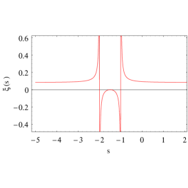
First of all, we have to find the physically acceptable range for , and the most important requirement is, of course, that , i.e. . This restricts to as shown in Fig.(1).
As mentioned above in the range the potential is of an inverse power-law type,
. In this case our model naturally admits
cosmological scaling solutions, recently studied, for example by
(Amendola (1999); Uzan (1999)) in the context of quintessence models. In
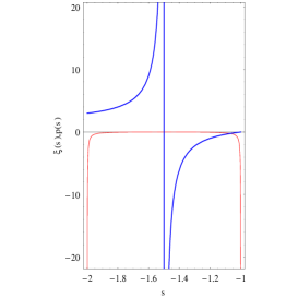
Fig.(2) we see that all the possible exponents for the
inverse power-law potential are available.
To determine the integration constants , and we follow the procedure used in Paper I, and we use the age of the universe, , as a unit of time. Because of our choice of time unit, the expansion rate is dimensionless, so that our Hubble constant is clearly of order 1 and is not (numerically) the same as the that is usually measured in . Setting and , we are able to express and as functions of and . We obtain:
| (21) | |||||
| (22) |
Therefore, our family of models, labeled by , depends only on , and . For both these parameters we have not only a thorough knowledge of their physical meaning, but for we can also strongly constrain its range of variability. Actually, we may easily obtain the relation
| (23) |
where as usual and is the age of the universe in Gy. We see that fixes only the product . In particular, we know that (see for instance Spergel & al. (2006)), thus for we get . The actual value of may be obtained by some of the subsequent tests or in others it has to be set as a prior - this will be specified in each case considered below.
Using the available observational data we can further constrain the
range of possible values of . Actually requiring that today
, as indicated by observations of supernovae Ia and
WMAP, we constrain the range of possible values of to .
From the Eqs. (14) and (15) it turns out
that for small values of the scale factor and the scalar field
behave as
| (24) | |||||
| (25) |
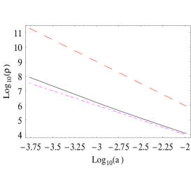
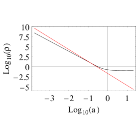
Substituting these functions in , as given by the Eq.(4), we get that for small the scalar field density . This is however true only asymptotically for very small . Exact computation as shown in Fig. (3) gives , with . This justifies our assertion that our model naturally admits scaling solutions. The situation changes dramatically near the present time (see below).
For large values of the scale factor and the scalar field behave as
| (26) | |||||
| (27) |

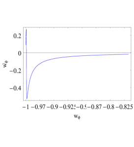
respectively, as shown in (Marino & de Ritis (2001)), where this asymptotical regime is discussed. It is interesting to note, as shown in Paper I, that is representing an equation of state, in the usual sense, of the effective cosmological constant , and that asymptotically behaves as a true cosmological constant () as . Let us also mention that since both and depend on through its time derivative (see Eqs. (4) and (3)) and asymptotically we recover in this limit the minimally coupled theory. In Figs. (4) and (5) we show the evolution with the redshift and the rate of evolution of ; the fast transition toward appears between and . Before reaching this asymptotic regime the energy density is dominated by the coupling term . Concluding this section we present the traditional plot - and compare it with the evolution of matter density (see Fig. (6)). It is interesting to see that follows the matter density during the matter dominated era, and it becomes dominant at late time.
3 Newtonian limit and Parametrized Post Newtonian (PPN) behaviour
Recently the cosmological relevance of extended gravity theories, as scalar tensor or higher order theories, has been widely explored. However, in the weak field approximation, all these classes of theories are expected to reproduce the Einstein general relativity which, in any case, is experimentally tested only in this limit. This fact is a matter of debate since several relativistic theories do not reproduce Einstein results at the Newtonian approximation but, in some sense, generalize them, giving rise, for example, to Yukawa -like corrections to the Newtonian potential which could have interesting physical consequences. Moreover, in general, any relativistic theory of gravitation can yield corrections to the Newton potential (see for example, Will (1993)) which in the post–Newtonian (PPN) formalism could furnish tests for such theory, mainly based on the Solar System experiments. In this section we want to discuss the Newtonian limit of our class of scalar -tensor theories of gravity, the induced gravity theories, and to study the Parametrized Post Newtonian (PPN) behaviour of these theories.
In particular, it turns out that the Newtonian limit depends on . Furthermore, we find a quadratic correction to the Newtonian potential strictly depending on the presence of the scalar–field potential which acts as a cosmological constant.
3.1 Newtonian limit
In order to recover the Newtonian limit of our theory described by the action in Eq. (1), associated with the effective stress-energy tensor
| (28) |
where is the usual stress-energy tensor of matter and is the d’Alembert operator, we write the metric tensor as
| (29) |
where is the Minkowski metric and is a small correction. In the same way, we define the scalar field as a perturbation, of the same order as , of the original field , that is
| (30) |
where is a constant of order unity. It is clear that for and the standard Einstein general relativity with is recovered.
To write the Einstein tensor in an appropriate form, we define the auxiliary fields
| (31) |
and
| (32) |
where . Given these definitions, to the first order in , we obtain
| (33) |
where . To obtain the weak–field limit of the field equations we have also to expand the effective stress–energy tensor: this means that it is necessary to expand the coupling function and the self interacting potential. Specifically, it turns out that expanding the coupling function and the self–interacting potential (by using their explicit forms) up to the second order in , we get
| (34) |
| (35) |
where . Then, to the first order, the effective stress–energy tensor becomes
| (36) |
and the field equations assume the form
| (37) |
When describes a point particle of mass and for and we get
| (38) | |||||
| (39) | |||||
| (40) |
where only terms linear in are given and we omitted the constant terms.
3.2 Constraints on PPN parameters
A satisfactory description of the PPN limit for scalar tensor theories has been developed in (Esposito-Farese (2004); Damour & al. (1993)). In these papers, this limit has been thoroughly discussed leading to interesting results even in the case of strong gravitational sources like pulsars and neutron stars where the deviations from General Relativity are considered in a non-perturbative regime (Damour & al. (1993)). The starting point of such an analysis is a redefinition of the non minimally coupled Lagrangian action in terms of a minimally coupled scalar field model via a conformal transformation of the form . In fact, assuming the transformation rules:
| (41) |
and
| (42) |
one rewrites the action as
| (43) |
The first consequence of such a transformation is that the non-minimal coupling is transferred to the ordinary matter sector, introducing an interaction term between matter and the scalar field. Actually, the Lagrangian depends not only on the conformally transformed metric and the matter fields but it also depends on the coupling function. In the same way, the field equations can be recast in the Einstein frame. The energy-momentum tensor is defined as and is related to the Jordan expression as . Possible deviations from the standard General Relativity can be tested through the Solar System experiments (Will (1993)) and binary pulsar observations which give an experimental estimate of the PPN parameters. The generalization of these quantities to the scalar-tensor theories allows the PPN-parameters to be expressed in terms of the non-minimal coupling function , and in our case using the Eqs. (12) and (13), we obtain :
| (44) |
| (45) |
The above definitions imply that the PPN-parameters in general depend on the non-minimal coupling function and its derivatives. However in our model depends only on while . The PPN-parameters can be directly constrained by the observational data. Actually, Solar System experiments give accurate indications on the ranges of 111We indicate with the subscript 0 that the estimates are based on Solar System observations. .
| Mercury Perih. Shift (Shapiro (1993)) | |
|---|---|
| Lunar Laser Rang. (Williams & al. (1996)) | |
| Very Long Bas. Int. (Shapiro & al. (2004)) | |
| Cassini spacecraft (Bertotti, Iess & Tortora 2003 ) |
We summarize the experimental results in Table1. These results have been used by (Schimd, Uzan & Riazuelo (2005)) to set the following constrains :
| (46) |
It turns out that the limit for in the Eq. (46) is naturally verified, for each value of , while the constraint on is satisfied only for , as shown in Fig. (7).
For the sake of completeness, here we take into account even the shift that the scalar-tensor gravity induces on the theoretical predictions for the local value of the gravitational constant as coming from the Cavendish-like experiments. This quantity represents the gravitational coupling measured when the Newton force arises between two masses :
| (47) |
In the case of scalar tensor gravity, the Cavendish coupling is related to and and is given by :
| (48) |
and in our models it depends only on
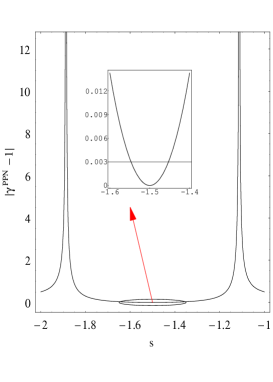
Finally, in Fig. (8) we plot the Brans-Dicke parameter as a function of : actually, for our model . It turns out that just for , satisfies the limits coming both from the Solar System experiments, (Will (1993)), and current cosmological observations, including cosmic microwave anisotropy data and the galaxy power spectrum data, give (Acquaviva & al. (2005)).222 It is worth noting that the legitimacy of the procedure of direct comparison of local and cosmological observations, in order to estimate variations of the physical constants, is a rather strong assumption, which deserves a proof or at least a justification. There is actually no reason a priori why local experiments should reveal variations occurring on cosmological scales, and in regions which are participating in the Hubble expansion. This interesting aspect of scalar tensor theories of gravity is discussed in (Clifton, Mota & Barrow (2005)) and in (Shaw & Barrow (2005)), where it is shown that such procedure is correct.

.
4 Some considerations about conformal transformations and interacting dark energy
Conformal transformations are often used to convert the non minimally coupled scalar field models into the minimally coupled ones, to gain mathematical simplification. The Jordan frame, in which the scalar field is nonminimally coupled to the Ricci curvature, is mapped into the Einstein frame in which the transformed scalar field is minimally coupled but at a price of coupling matter to the scalar field. The two frames are not physically equivalent, and some care has to be taken in applying this technique (see for instance (Faraoni (2000)) for a critical discussion about this point). In this section we study the effect of conformal transformations on our models and show that, in presence of matter, it can mimic a coupling between the quintessence scalar field and dark matter. We discuss some implications of such a fictitious interaction on the effective equation of state. Actually it turns out that, since the interaction alters the redshift-dependence of the matter density, it is possible to obtain an effective transformed dark energy equation of state of . Let us start from the transformation rules connected with the conformal transformation :
| (49) | |||||
| (50) | |||||
| (51) | |||||
| (52) |
with these new variables the Lagrangian in the Eq.(2) becomes
| (53) |
where now dot denotes derivative with respect to , and
| (54) |
An observer in the Einstein frame would infer that the scalar field is coupled to the dark matter, and this interaction is represented by the term , as it can be seen more clearly from the field equations:
| (55) | |||
| (56) |
where is the actual matter density (treated here as dust), the value of today, and . It turns out that the density of dark matter does not evolve as , but scales as . Also the Klein-Gordon equation (55) differs from the standard one because of the last term on the right hand side.
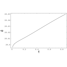
As shown in (Das et al. (2005)) interaction between dark matter and dark energy could result in an effective equation of state , mimicking the CDM model. Actually is defined by the matter continuity equation
| (57) |
where
| (58) |
It can be shown that is simply related to
| (59) |
where
| (60) |
Since today, one has , which is greater than or equal to . It turns out (Das et al. (2005)), however, that increases in time, so that and it is possible to have in the past. In such a way interaction between dark matter and dark energy could generate a superquintessence regime, provided that the observer treats the dark matter as non-interacting, and ascribes part of the dark matter density to the scalar field, as is shown in Eq. (58). On the other hand an interacting dark energy component could hide the effect of a non standard gravity, in the Einstein frame, provided that it is considered as the physical one.

4.1 Conformally transformed coupled dark energy
Let us consider our nonminimally coupled model characterized by the functions and respectively. According to the rules in Eqs. (49 - 52) we obtain the following relations between the transformed and original dynamical quantities:
| (61) | |||||
| (62) | |||||
| (63) |
As we see from Eq. (62), in the transformed frame the cosmic evolution is mediated by the presence of the scalar field. The explicit form of Eq. (51), which connects the cosmic time in both frames, can be written in analytical form, but is indeed rather complicated: actually it turns out that
| (64) | |||||
From the Eqs. (61–64) we can evaluate the scalar field energy density and pressure, and the equation of state according to the usual definitions.
As in the Jordan frame, it turns out that also in the Einstein frame for (see for instance Fig. (10)).
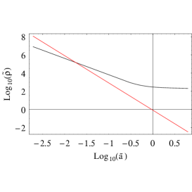
Concluding this section we present the traditional plot - and compare it with - relation (see Fig. (11)). Interestingly we see that, just because of the interaction term, does not track anymore the matter during the matter dominated era, as it happens in the Jordan frame (see Fig. 6), but becomes dominant at earlier times.
4.2 Non minimally coupled quintessence and mass varying neutrinos through conformal transformations
In this section we briefly discuss how the scalar tensor theories of gravity could be involved in a cosmological model with mass varying neutrinos that mimic the dark energy, a quite different theoretical scenario of evolution of the universe that recently has been suggested by (Fardon & al. (2004)). Let us recall that recently the mass differences between neutrino mass eigenstates (, , ) have been measured in oscillation experiments (Lesgourgues and Pastor (2006)). Observations of atmospheric neutrinos suggest a squared mass difference of , while solar neutrino observations, and results from the KamLAND neutrino experiment, point towards . While only weak constraints on the absolute mass scale () have been obtained from single -decay experiments, the double beta decay searches from the Heidelberg-Moscow experiment have reported a signal for a neutrino mass at level ( Klapdor-Kleingrothaus and al. (2004)), recently promoted to level (Klapdor-Kleingrothaus (2006)). This last result translates into a total neutrino mass of at c.l., but this claim is still considered as controversial (see Elliott and Engel (2004)). It is known in the literature (Lesgourgues and Pastor (2006)) that massive neutrinos can be extremely relevant for cosmology as they leave key signatures in several cosmological data sets. More specifically, massive neutrinos suppress the growth of fluctuations on scales below the horizon scale when they become non relativistic. Current cosmological data have been able to indirectly constrain the absolute neutrino mass to eV at c.l. (Spergel & al. (2006)), and are challenging the Heidelberg-Moscow claim. However, as first noticed by (Hannestad (2005)), there is some form of anticorrelation between the equation of state parameter and . The cosmological bound on neutrino masses can therefore be relaxed by considering a dark energy component with a more negative value of than a cosmological constant. Actually it has been proved that the Heidelberg-Moscow result is compatible with the cosmological data only if the equation of state (with being constant) is at . This result suggests an interesting link between neutrinos and dark energy (see for instance Brookfield & al. 2005 b ; Brookfield & al. 2005 a ; Bi & al. (2004); Kaplan & al. (2004); Amendola (2004)). According to this scenario the late time accelerated expansion of the universe is driven by the coupling between the quintessential scalar field and neutrinos. Due to such coupling the mass of neutrinos becomes a function of this scalar field. Since the scalar field evolves with time the mass of neutrinos is not constant (mass-varying neutrinos): the main theoretical motivation for such connection relies on the fact that the energy scale of the dark energy is of the order of the neutrinos mass scale. Moreover, as discussed above, in interacting dark energy models, the net effect of the interaction is to change the apparent equation of state of the dark energy, allowing a so called superquintessence regime, with . Interestingly enough, if the Heidelberg-Moscow results are combined with the WMAP 3-years data and other independent cosmological observations, as the ones connected with the large scale structure – coming from galaxy redshift surveys and Lyman- forests, or with the SNIa surveys, it is possible to constrain the equation of state to at c.l., ruling out a cosmological constant at more than c.l. (see De La Macorra et al. (2007)).
In the following we will discuss the coupling between neutrinos and dark energy from the point of view of the conformal transformation, according to the arguments outlined in the previous section, i.e. we will show that the neutrino mass and scalar field coupling can be interpreted as an effect of conformal transformations from the Jordan to the Einstein frame, just as it happens for the coupling between the dark energy and the dark matter. For our purpose the neutrinos can be either Dirac or Majorana particles, the only necessary ingredient is that, according to (Fardon & al. (2004)), the neutrino mass is a function of the scalar field. In the cosmological context, neutrinos should be treated as a gas (Brookfield & al. 2005 b ) and described by the collisionless distribution function in the phase space (where is the conformal time) that satisfies the Boltzmann equation. When neutrinos are collisionless the distribution function does not depend explicitly on time. We can solve then the Boltzmann equation and calculate the energy density stored in neutrinos ( is the background neutrino distribution function):
| (66) |
with , is the scale factor and is the comoving momentum. The pressure is
| (67) |
From these equations we derive that
| (68) |
(note that here the dot denotes the derivative with respect to ). The Klein Gordon equation for the scalar field reads
| (69) |
We see that Eq. (69) is formally equivalent to Eq. (55), but now the term on the right hand side describes coupling of the scalar field to the neutrino mass. As shown above the interaction between neutrinos and dark energy could result in an effective equation of state , defined in Eq.( 57), while is defined in the standard way by . As in the previous section the parameter is related to by
| (70) |
with
| (71) |
Also in this case can be less than , as was pointed out in the context of models with dark matter/dark energy interaction. This circumstance could lead to an observational test to establish which of the frames, Jordan or Einstein, is the physical one, since the coupling between the quintessential scalar field is provided by the function , which should drive not only the dark matter evolution (see Eq. (55)), but also the neutrinos mass variation and the evolution of the gravitational constant .
5 Observational data and predictions of our models

5.1 Constraints from recent SNIa observations
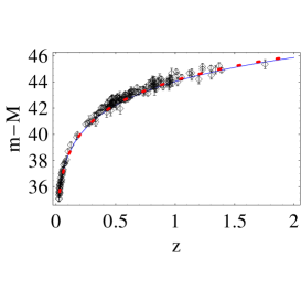
In this section we present results of fits of predictions of our model to the best SNIa data sets presently available. As a starting point we consider the sample of 182 SNIa compiled in (Riess et al. (2007)), which includes the 21 new Type Ia supernovae recently discovered with the Hubble Space Telescope (HST), and combines previous SNIa data sets, namely the Gold Sample compiled in (Riess & al. (2004)) supplemented by the SNLS data set (Astier & al. (2005)). Following the procedure described in Paper I, we perform a analysis comparing the redshift dependence of the theoretical values to the observational estimates of the distance modulus, , which in scalar tensor theories of gravity takes the form
| (72) |
Here the presence of the correction term
| (73) |
describes the effect of time variation of the effective gravitational constant on the luminosity of high redshift supernovae, and allows one to test the scalar tensor theories of gravity (Gaztañaga & al. 2001 ; Uzan (2003)) using the SNIa data. Moreover, for a general flat and homogeneous cosmological model the luminosity distance can be expressed as an integral of the Hubble function as follows:
| (74) |
where is related to the Hubble function expressed in terms of . Let us note that the luminosity distance depends also on the Hubble distance ( which does not depend on the choice of the unit of time). Such freedom allows us to fit or the a priori unknown age of the universe using the SNIa dataset. We find that for 182 data points, and the best fit values are , , which corresponds to . We also get .
In Fig (13) we compare the best fit curve with the observational data sets.
5.1.1 Dimensionless coordinate distance test
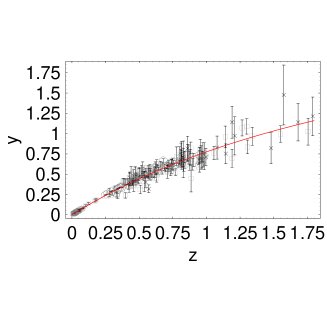
After having explored the Hubble diagram of SNIa, let us now follow the more general approach, suggested by Daly & Djorgovski (Daly & Djorgovski (2004)), and already tested in Paper I. Consider as a cosmological observable the dimensionless coordinate distance defined as :
| (75) |
noting that does not depend explicitly on , so that any choice for does not alter the main result. Daly & Djorgovski have determined for the SNIa in the Gold Sample of Riess et al. (Riess & al. (2004)) which is the most homogeneous SNIa sample available today. Since SNIa allows to estimate rather than , a value of has to be set. Fitting the Hubble law to a large set of low redshift () SNIa, Daly & Djorgovski (Daly & Djorgovski (2004)) have set:
To enlarge the sample, Daly & Djorgovski added 20 points on the diagram using a technique of distance determination based on the angular dimension of radiogalaxies (Daly & Djorgovski (2004)). This data set has been recently supplemented by 71 new supernovae from the Supernova Legacy Survey of (Astier & al. (2005)), which allowed the determination of dimensionless coordinate distances to these supernovae. These were obtained using the values and uncertainties of listed in Table 9 of (Astier & al. (2005)), with . This extended sample that spans the redshift range has been suitably homogenized.
Using the following merit function :
| (76) |
we obtain that for 248 data points, and the best fit values are , . In Fig (14) we compare the best fit curve with the observational data set, as in Paper I.
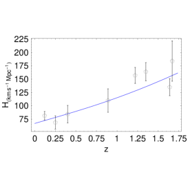
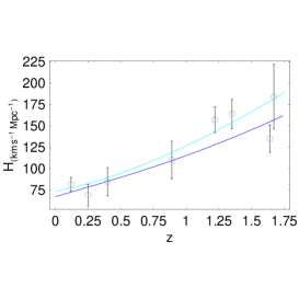
5.1.2 H(z) and the relative galaxy ages
In this section we discuss a possible observational determination of based on the method developed by (Jimenez & al. 2003) ), that involves differential age measurements. We present some constraints that can be placed on the evolution of our quintessence model by such data. First, it is worth to stress some aspects connected with the sensitivity of the cosmology to the and relations. Actually, it is well known that in scalar tensor theories of gravity, as well as in general relativity, the expansion history of the universe is determined by the function . This implies that observational quantities, like the luminosity distance, the angular diameter distance, and the lookback time, all depend on . It turns out that the most appropriate mathematical tool to study the sensitivity of the cosmological model to such observables is the functional derivative of the corresponding relations with respect to the cosmological parameters (see Saini, Padmanabhan & Bridle (2003) for a discussion about this point in relation to distance measurements).
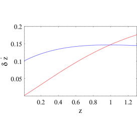
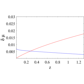
However, also from an empirical point of view, it is possible to show that the lookback time is much more sensitive to the cosmological model than other observables, like the luminosity distance, and the distance modulus. This circumstance encourages us to use, together with other more standard techniques discussed above, the age of cosmic clocks to test alternative cosmological scenarios. Apart from the advantage of providing an alternative instrument of investigation, the age-based methods use the stronger sensitivity to the cosmological parameters of the relation, as shown in Figs. (15) and (16). Moreover, as we will discuss in the following, such a method reveals its full strength when applied to old objects at very high . Actually it turns out that this kind of analysis could remove, or at least reduce, the degeneracy which we observe at lower redshifts, for example the one in the Hubble diagram for SNIa observations, which can be fitted by different cosmological models with similar statistical significance. Since the Hubble parameter can be related to the differential age of the universe as a function of redshift by the equation
| (77) |
a determination of directly measures . Jimenez et al. ( Jimenez & al. 2003) ) demonstrated the feasibility of this method by applying it to a sample of galaxies. With the availability of new galaxy surveys it becomes possible to determine at . Here we use the data from (Simon & al. 2005) ) to determine in the redshift range . To follow the procedure described in (Simon & al. 2005) ), first we group together all galaxies that are within of each other. This gives an estimate of the age of the universe at a given redshift. We then compute age differences only for those bins in redshift that are separated by more than but less than . The first limit is imposed so that the age evolution between the two bins is larger than the error in the age determination. We note here that differential ages are less sensitive to systematic errors than absolute ages (see Jimenez & al. 2003) ). The observational value of is then directly computed by using Eq. (77), and after that the ages data have been scaled according to our choice of the unit of time (the unknown scaling factor has been provided by the procedure). To determine the best fit parameters, we define the following merit function :
| (78) |
We obtain that for 9 data points, and the best fit values are , . In Fig (17) we compare the best fit curve with the observational data set.
5.2 The Sunyaev-Zeldovich/X-ray method
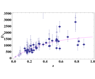
In this section we discuss how the parameters of our model can be constrained by the angular diameter distance as measured using the Sunyaev-Zeldovich effect (SZE) and the thermal bremsstrahlung (X-ray brightness data) for galaxy clusters. The distance measurements using Sunyaev-Zeldovich effect and X-ray emission from the intracluster medium have to take into account that these processes depend on different combinations of some of the parameters of the clusters (see Birkinshaw (1999) and references therein). The SZE is a result of the inverse Compton scattering of the CMB photons on hot electrons of the intercluster gas, which preserves the number of photons, but allows photons to gain energy and thus generates a decrement of the temperature in the Rayleigh-Jeans part of the black-body spectrum while an increment appears in the Wien region. We limit our analysis to the so called thermal or static SZE. The effect, present only in clusters with a nonzero peculiar velocity with respect to the Hubble flow along the line of sight, will be neglected since typically the thermal SZE is an order of magnitude larger than the kinematic one. As in Paper I, we introduce the so called Compton parameter, , defined as the optical depth times the energy gain per scattering:
| (79) |
where is the temperature of the electrons in the intracluster gas, is the electron mass, is the number density of the electrons, and is the Thompson cross section of electron scattering, and the integration is performed along the line of sight. In the low frequency regime of the Rayleigh-Jeans approximation the shift of temperature is
| (80) |
where is the unperturbed CMB temperature. The next step to quantify the SZE decrement is to specify the model for the intracluster electron density and temperature distribution, which appropriately describes the observational properties of the gas. Following (Bonamente & al. (2005)) we use a hydrostatic equilibrium double -model model. Actually, at the center of clusters the density may be high enough that the radiative cooling time-scale is less than the cluster’s age, leading to a reduction in temperature and an increase in central density. This can increase the central X-ray emissivity. At large radii, the density of the gas is sufficiently low that X-ray emission can be sustained for cosmological periods without significant cooling. Therefore, cool core clusters effectively exhibit two components: a centrally concentrated gas peak and a broad, shallower distribution of the gas. This phenomenon motivated the modelling of the gas density with a function of the form:
| (81) |
The quantity is the central density, governs the fractional contributions of the narrow and broad components (), and are the two core radii that describe the shape of the inner and outer portions of the density distribution and determines the slope at large radii (the same is used for both the central and outer distribution in order to reduce the total number of degrees of freedom) 333It is worth to note that there are also different hydrodynamical models which predict universal gas density and gas temperature profiles that agree with the observations (see for instance the one illustrated in (Komatsu & Seljak (2001)), derived from the universal dark matter density profile, assuming that the gas density traces the dark matter density in the outer parts of halos, or the one introduced in (Rasia, Tormen, Moscardini (2004))).. This shape generalizes the single -model profile, introduced by Cavaliere and Fusco-Femiano (1976) and commonly used to fit X-ray surface brightness profiles, to a double -model of the density that has the freedom of following both the central spike in density and the more gentle outer distribution. A double -model of the surface brightness was first used by Mohr et al. (1999) to fit X-ray data of galaxy clusters; the density model of Eq. (81) was further developed by La Roque (La Roque et al. (2006)). The X-ray surface brightness is related to the gas density as
| (82) |
where is the cluster redshift, is the X-ray cooling function, and it is a function of plasma temperature and energy in the rest frame of the cluster, including contributions from relativistic electron-ion thermal bremsstrahlung, electron-electron thermal bremsstrahlung, recombination, and two photon processes. The cluster angular diameter distance , where is the line-of-sight angular size, can be inferred with a joint analysis of SZE, taking advantage of the different density dependence of the X-ray emission and SZE decrement:
| (83) | |||
Actually it turns out that
| (84) |
Note that is proportional to and (since ), so the distance determination is strongly dependent on the accuracy of the SZE decrement and X-ray temperature measurements.
Recently distances to 18 clusters with redshift ranging from to have been determined from a likelihood joint analysis of SZE and X-ray observations (see Table 7 in Reese & al. (2002)). We perform our analysis using angular diameter distance measurements for a sample of 83 clusters, containing the 18 above mentioned clusters, other 24 known previously (see Birkinshaw (1999)), and a recently released sample with the measurement of the angular diameter distances from the Chandra X-ray imaging and Sunyaev-Zel’dovich effect mapping of 39 high redshift clusters of galaxies ( ) (Bonamente & al. (2005)). The unprecedented spatial resolution of Chandra combined with its simultaneous spectral resolution allows a more accurate determination of distances. Let us consider the merit function of the form :
| (85) |
Fitting the data we obtain that for 83 data points, and the best fit values are , and . In Fig. (19) we compare the best fit curve with the observational SZE data.
5.3 Gamma-Ray Burst Hubble Diagram
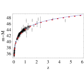
Gamma-ray bursts (GRBs) are bright explosions visible across most of the Universe, certainly out to redshifts of and likely out to . Recent studies have pointed out that GRBs may be used as standard cosmological candles (Ghirlanda & al. (2004); Friedman & Bloom (2005)): actually it turns out that the energy released during bursts spans nearly three orders of magnitude, and the distribution of the opening angles of the emission, as deduced from the timing of the achromatic steepening of the afterglow emission, spans a similar wide range of values. However, when the apparently isotropic energy release and the conic opening of the emission are combined to infer the intrinsic, true energy release, the resulting distribution does not widen, as is expected for uncorrelated data, but shrinks to a very well determined value (Frail & Kulkarni (2003)), with a remarkably small (one–sided) scattering, corresponding to about a factor of in total energy. Similar studies in the X–ray band have reproduced the same results. It is thus very tempting to study to what extent this property of GRBs makes them suitable cosmological standard candles. Schaefer (Schaefer (2003)) proposed to use the two well known correlations of the GRBs luminosity (with variability, and with time delay), while others exploited the recently reported relationship between the beaming–corrected -ray energy and the locally observed peak energy of GRBs (see for instance Dai & al. (2004)). As for the possible variation of ambient density from burst to burst, which may widen the distribution of bursts energies, Frail & Kulkarni (Frail & Kulkarni (2003)) remarked that this spread is already contained in their data sample, and yet the distribution of energy released is still very narrow. There are at least two reasons why GRBs are better than type Ia supernovae as cosmological candles. On the one hand, GRBs are easy to find and locate: even 1980s technology allowed BATSE to locate 1 GRB per day, making the build–up of a 300–object database a one–year enterprise. The Swift satellite launched on 20 November 2004, detects GRBs at about the same rate as BATSE, but with a nearly perfect capacity for identifying their redshifts simultaneously with the afterglow observations 444http://swift.gsfc.nasa.gov. Second, GRBs have been detected out to very high redshifts: even the current sample contains several events with , with one (GRB 000131) at and another at . This should be contrasted with the difficulty of locating SN at , and absence of any SN with . On the other hand, the distribution of luminosities of SNIa is narrower than the distribution of energy released by GRBs, corresponding to a magnitude dispersion rather than . Thus GRBs may provide a complementary standard candle, out to distances which cannot be probed by SNIa, their major limitation being the larger intrinsic scatter of the energy released, as compared to the small scatter in peak luminosities of SNIa. There currently exists enough information to calibrate luminosity distances and independent redshifts for nine bursts (Schaefer (2003)). These bursts were all detected by BATSE with redshifts measured from optical spectra of either the afterglow or the host galaxy. The highly unusual GRB980425 (associated with supernova SN1998bw) is not included because it is likely to be qualitatively different from the classical GRBs. Bursts with red shifts that were not recorded by BATSE cannot yet have their observed parameters converted to energies and fluxes that are comparable with BATSE data. For the present analysis we shall use a sample of GRBs that had their redshifts estimated (Bloom, Frail & Kulkarni (2003)), as represented by empty boxes in Fig. (20), with the distance modulus , given by Eq. (72).
To this aim, the only difference with respect to the SNIa is that we slightly modify the correction term of Eq. (73), and we take
| (86) |
We expect that is of order unity, so that the -correction would be roughly half a magnitude. We obtain for data points, and the best fit value is , , which are compatible with the SNIa results. We also find that which appears in Eq. (86) is equal to . In Fig. (20) we compare the best fit curve with both the GRBs and the SNIa Gold Sample.
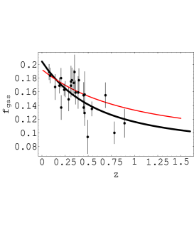
5.4 The gas fraction in clusters
Measurements of the gas mass fraction in galaxy clusters have been proposed as a test of cosmological models (Allen & al. (2002)). Both theoretical arguments and numerical simulations predict that the baryonic mass fraction in the largest relaxed galaxy clusters should not depend on the redshift, and should provide an estimate of the cosmological baryonic density parameter (Eke & al. (1998)). The baryonic content in galaxy clusters is dominated by the hot X - ray emitting intra-cluster gas so that what is actually measured is the gas mass fraction and it is this quantity that should not depend on the redshift. Moreover, it is expected that the baryonic mass fraction in clusters is equal to the universal ratio so that should indeed be given by , where the multiplicative factor is motivated by simulations that suggest that the gas fraction is lower than the universal ratio. Following the procedure described in (Allen & al. (2002, 2004)), and already used in Paper I we adopt the standard CDM model (i.e., a flat universe with and ) as a reference cosmology in making the measurements so that the theoretical expectation for the apparent variation of with the redshift is:
| (87) |
where we substitute the appropriate expression of for our model, and and are the angular diameter distance for the SCDM and our model respectively. Allen & al. (Allen & al. (2002)) have extensively analyzed the set of simulations in (Eke & al. (1998)) to get , so in our analysis below, we set . Actually, we have checked that, for values in the range quoted above, the main results do not depend on . Moreover we have defined the following merit function :
| (88) |
where
| (89) |
Here is the measured gas fraction in galaxy clusters at redshift with an error and the sum is over the clusters considered. Let us note that recently Allen & al. (Allen & al. (2004)) have released a catalog of 26 large relaxed clusters with a precise measurement of both the gas mass fraction and the redshift . We use these data to perform our likelihood analysis, we get for 26 data points, and , , , and . A brief comparison of our results with similar recent results of Lima et al. (Lima & al. (2003)), where the equation of state characterizing the dark energy component is constrained by using galaxy clusters x-ray data, can still be done. In their analysis, however, they consider quintessence models in the standard gravity theories, with a non evolving equation of state, but they allow the so-called phantom dark energy with , which violates the null energy condition. As the best fit value of to the data of (Allen & al. (2002)) they obtain . In order to directly compare this result with our analysis we first fit the model considered in (Lima & al. (2003)) to the updated and wider data set of (Allen & al. (2004)), used in our analysis. To this aim we also refer to the model function , and the merit function , defined in the Eqs. (87) and (88) respectively. We get for 26 data points, and , , and , so , what corresponds to a phantom energy. Let us note that our model, instead, gives , what does not violate the null energy condition. In Fig. (21) we compare the best fit curves for our and the Lima & al. model with the observational data.
6 Growth of density perturbations
In this section we consider the evolution of scalar density perturbations in the longitudinal gauge . Contrary to what happens in the framework of the minimally coupled theory, where we have to deal with a fully relativistic component, which becomes homogeneous on scales smaller than the horizon – so that standard quintessence cannot cluster on such scales – in the non minimally coupled quintessence theories it is possible to separate a pure gravitational term both in the stress-energy tensor , and in the energy density , so the situation changes, and it is necessary to consider also fluctuations of the scalar field. However, it turns out (Boisseau & al. 2000 ; Riazuelo & Uzan (2002)) that the equation for dust like matter density perturbations inside the horizon can be written as follows:
| (90) |
where is the effective gravitational constant defined by
| (91) |
The equation (90) describes, in the non minimally coupled models, evolution of the CDM density contrast, , for perturbations inside the horizon. In our model the Eq.(90) is rather complicated and takes the form
| (92) | |||||
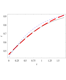
Eq. (92) does not admit exact solutions, and can be solved only numerically. However, since with our choice of normalization the whole history of the Universe is confined to the range and therefore to study the behavior of solutions for we can always expand the functions in Eq. (92) in series around , in order to get approximate solutions. Actually we obtain an integrable Fuchsian differential equation, which is a hypergeometric equation. We then use such a solution to set the initial conditions at to numerically integrate Eq. (92) in the whole range . We use the growing mode and define the growth index as
| (93) |
where is the scale factor. Once we know how the growth index evolves with redshift and how it depends on our model parameters, we can use the available observational data to estimate the values of such parameters, and the present value of . The 2dFGRS team has recently collected positions and redshifts of about galaxies and presented a detailed analysis of the two-point correlation function. They measured the redshift distortion parameter , where is the bias parameter describing the difference in the distribution of galaxies and mass, and obtained that and . From the observationally determined and it is now straightforward to get the value of the growth index at corresponding to the effective depth of the survey. Verde & al. (Verde & al. (2001)) used the bispectrum of 2dFGRS galaxies, and Lahav & al. (Lahav & al. (2002)) combined the 2dFGRS data with CMB data, and they obtained
| (94) | |||||
| (95) |
Using these two values for we calculated the value of the growth index at , we get respectively
| (96) | |||||
| (97) |
To evaluate the growth index at we first have to invert the relation and find : actually the relation is rather involved and cannot be analytically inverted, so we perform this inversion numerically. Finally, we get , which corresponds to . In Fig. (22) we show how the growth index is changing with redshift in our non minimally coupled model as compared with the standard -CDM model, with , and a quintessence model namely the minimally coupled exponential model described in (Demianski & al. (2005)). We note that at low redshift theoretical predictions of these different models are not distinguishable, independent measurements from large redshift surveys at different depths could disentangle this degeneracy.
7 Summary and conclusions
In this paper we have extended the analysis that we performed in Paper I (where we have analyzed a special extended quintessence model, based on one of the most commonly used quintessence potentials , corresponding to the coupling ), considering a new and wider class of theories for which exact solutions of the Einstein equations are known, and discussed how in such models it is possible to treat the fine tuning problem in an alternative way. We have shown that in the family of such models selected by requiring that their corresponding point like Lagrangian admits a Noether symmetry an epoch of accelerated expansion appears in a natural way. In the non minimally coupled scalar tensor theory of gravity it is possible to perform an appropriate conformal transformation and to move from the Jordan picture to the standard Einstein one but then matter becomes coupled to the scalar field. We have explored both descriptions and also considered the neutrino mass varying model as a possible example of non minimally coupled scalar tensor theory.
It turns out that the imposed requirement of existence of a Noether symmetry is quite restrictive and we obtained a family of models that is fully specified by 3 parameters: a parameter that determines the strength of the non minimal coupling and the potential of the scalar field, the Hubble constant, and a parameter that determines the scale of the potential. To determine the values of these parameters we compared predictions of our model with several independent observational data. The results of this parameter determination procedure are presented in Table 2. We see that with our average value of the scale factor, for small , is changing as , and for large , as while and in corresponding asymptotic regimes. The potential is decaying to zero for large , after reaching a maximum value, (see Fig. (23)). Similarly, the effective gravitational coupling is decreasing for large , until it becomes zero for ( we have a sort of asymptotic freedom at ). It turns out that in our model the observational constraints on the variation of the effective gravitational constant are respected. Actually a new analysis of the Big Bang Nucleosynthesis (Copi et al. (2004)) restricts the variations of to
| (98) |
at confidence level, where , and . The combined analysis of the new 4He and WMAP data implies that
| (99) |
A recent analysis of the secular variation of the period of nonradial pulsations of the white dwarf G117-B15A shows (Benvenuto et al. (2004)) that at 2, which is of the same order of magnitude as previous independent bounds (see also Biesiada & Malec (2004)). With our unit of time this becomes , where as given by the WMAP team (Spergel & al. (2006)).
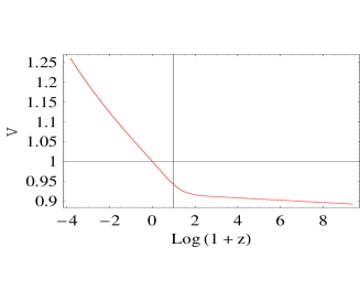
Initially, for small , the matter energy density is larger than the energy density of the scalar field.
In Table (2) we present results of our analysis, they show that predictions of our model are fully compatible with the recent observational data. Comparing results of this paper with our previous analysis of minimally coupled scalar field models (see Paper I) we conclude that the present day observational data connected with the post recombination evolution of the universe can be fitted by several different models of quintessence. More data on high redshift supernovae of type Ia and GRBs are needed as well as more information on the early phase of structure formation in order to place stronger restrictions on the allowed type of dark energy.
| dataset | ||||
|---|---|---|---|---|
| high redshift SNIa | ||||
| dimensionless coordinates test | ||||
| relative galaxy ages | ||||
| sze data | ||||
| GRBs dataset | ||||
| fraction of gas in clusters | ||||
| galaxies peculiar velocity | ||||
| average |
Acknowledgments
This work was supported in part by the grant of Polish Ministry of Science and Higher Education 1-P03D-014-26, and by INFN Na12. The authors are very grateful to Professor Djorgovski, for providing the data that we used in Sec. 3.1.1, and to Professors Verde and Simon, for providing the data used in Sec. 3.2.2. Of course we take full responsibility of the fitting procedure.
References
- Accetta et al. (1984) Accetta F.S., Zoller D.J.,Turner M.S., 1985, Phys. Rev. D 31, 3064
- Acquaviva & al. (2005) Acquviva V., & al., 2005, Phys.Rev. D 71 104025
- Allen & al. (2002) Allen S.W., Schmidt R.W., Fabian A.C., 2002, MNRAS, 334, L11
- Allen & al. (2004) Allen S.W., & al. 2004, MNRAS, 335, 457
- Amendola (1999) Amendola L., 1999, Phys.Rev. D 60 043501
- Amendola (2004) Amendola L., Gasperini M., and Piazza F., 2004, JCAP 9, 014
- Astier & al. (2005) Astier P., & al., 2006, A&A, 447, 31; astro-ph/0510447
- Benvenuto et al. (2004) Benvenuto O.G., Garcia-Berro E. , and Isern J., Phys. Rev. D, 2004, 69, 082002
- (9) Bertotti B., Iess L., Tortora P., 2003, Nature 425, 374
- Bi & al. (2004) Bi X.-J., Gu P., Wang X., Zhang X., 2004, Phys.Rev.D, 69, 113007
- Biesiada & Malec (2004) Biesiada M., and Malec B., 2004, MNRAS, 350, 644.
- Birkinshaw (1999) Birkinshaw, M., Phys. Rep.,1999, 310, 97.
- Bloom, Frail & Kulkarni (2003) Bloom J. S., Frail D. A. & Kulkarni S. R., 2003, ApJ, 594, 674
- Bonamente & al. (2005) Bonamente M., & al., 2005, astro-ph/0512349
- (15) Brookfield A. W. & al., 2006, Phys. Rev. D73, 083515; astro-ph/0512367
- (16) Brookfield A. W. & al., 2006, Phys. Rev. Lett., 96, 061301; astro-ph/0503349
- (17) Boisseau B., Esposito-Farese G., Polarski D., Starobinsky A.A., 2000, Phys. Rev. Lett., 85, 2236
- Caldwell, Dave & Steinhardt (1998) Caldwell R.R., Dave R., Steinhardt P.J., 1998, Phys. Rev. Lett., 80, 1582
- Caldwell, Kamionkowski& Weinberg (2003) Caldwell R.R., Kamionkowski M., Weinberg N.N., 2003, Phys.Rev.Lett., 91, 071301
- Capozziello & al. (1996) Capozziello S., de Ritis R., Rubano C., and Scudellaro P., 1996, Riv. del Nuovo Cimento 19, vol. 4 (1996)
- Capozziello et al. (1996) Capozziello S., de Ritis R., Marino A. A., 1997, Class.Quant.Grav., 14,3243
-
(22)
Cavaliere A.,Fusco–Femiano R., 1976, 49 (1976) 137;
Cavaliere A.,Fusco–Femiano R., 1978, A&A, 70 (1978) 677 - Clifton, Mota & Barrow (2005) Clifton T., Mota D.F., Barrow J.D., 2005, MNRAS, 358, 601
- Copi et al. (2004) Copi C.J.,Davis A.N., and Krauss L.M., 2004, Phys. Rev. Lett.,92, 171301
- Crooks & Frampton (2005) Crooks J. L. & Frampton P.H., 2005 astro-ph/0601051
- Cyburt et al. (2004) Cyburt R.H. et al., astro-ph/0408033.
- Dai & al. (2004) Dai Z. G., Liang E. W. & Xu D. 2004, ApJ 612 L101
- Daly & Djorgovski (2004) Daly R.A., Djorgovski S.G. 2004, ApJ, 612, 652
- Daly & Djorgovski (2005) Daly R., & Djorgovski S. G., 2005, astro-ph/0512576
- Das et al. (2005) Das S., Corasaniti P., & Khoury J., 2005, astro-ph/0510628
- De La Macorra et al. (2007) De La Macorra A., et al. 2007, Astroparticle Physics, 27, 406
- Demianski & al. (1991) Demianski M., de Ritis R., Marmo G., Platania G., Stornaoiolo C., 1991, Phys. Rev. D, 44, 3136
- Demianski & al. (2003) Demianski M., de Ritis R., Marino A.A., Piedipalumbo E., 2003, A&A, 411, 33
- Demianski & al. (2005) Demianski M., Piedipalumbo E., Rubano C., Tortora C., 2005, A&A,431, 27
- Demianski & al. (2006) Demianski M., Piedipalumbo E., Rubano C., Tortora C., 2006, A&A, 454, 55
- de Ritis & al. (2000) de Ritis R., Marino A.A., Rubano C., and Scudellaro P., 2000, Phys. Rev. D 62, 043506
- Damour & al. (1993) Damour T., Esposito-Farese G., 1993, Phys. Rev. Lett. 70, 2220
- Eke & al. (1998) Eke V., Navarro J.F., Frenk C.S., 1998, ApJ, 503, 569
- Elliott and Engel (2004) Elliott S.R. and Engel J., 2004, J.Phys. G 30, R 183
- Ellis et al. (1984) Ellis J. et al., 1984, Phys. Lett. B 134, 429
- Esposito-Farese (2004) Esposito Farese G., pre-print: gr-qc/0409081.
- Faraoni (2000) Faraoni V., 2000 Phys.Rev. D, 62, 023504
- Fardon & al. (2004) Fardon R., Nelson A. E. & Weiner N., JCAP 0410:005 (2004)
- Frail & Kulkarni (2003) Frail D. A. & Kulkarni S. R. 2003, ApJ, 594 674
- Friedman & Bloom (2005) Friedman A. S. & Bloom J. S., 2005, ApJ, 627, 1
- Garcia-Bellido (1997) Garcia-Bellido J., 1997, Phys. Rev. D 55, 4603
- (47) Gaztañaga E., Garcia-Berro E., Isern J., Bravo E., & Dominguez, 2001, Phys. Rev. D, 1 ????
- Ghirlanda & al. (2004) Ghirlanda G., Ghisellini G. & Lazzati D., 2004, ApJ, 616, 331
- Hannestad (2005) Hannestad S.,, 2005, Phys. Rev. Lett. 95, 221301
- Hu (2005) Hu W., 2005, Phys. Rev. D, 71, 047301
- (51) Jimenez R., Verde L., Treu T., Stern D., 2003, ApJ., 593, 622
- Kaplan & al. (2004) Kaplan D.B., Nelson A.E., & Weiner N., 2004, Phys.Rev.Lett. 93, 091801
- Klapdor-Kleingrothaus and al. (2004) Klapdor-Kleingrothaus H.V., Krivosheina I.V., Dietz A., and Chkvorets O., 2004, Phys. Lett. B 586, 198
- Klapdor-Kleingrothaus (2006) Klapdor-Kleingrothaus H.V., talk at SNOW 2006, 2nd Scandinavian Neutrino Workshop (Stockholm, Sweden, 2006).
- Komatsu & Seljak (2001) Komatsu E. & Seljak U., 2001, MNRAS, 327, 1353
- Lahav & al. (2002) Lahav O., Bridle S. L., Percival W. J., & the 2dFGRS Team, 2002, MNRAS, 333, 961
- La Roque et al. (2006) La Roque, S., Bonamente, M., Joy, M., Carlstrom, J., Nagai, D., Reese, E. and Dawson, K. 2006, ApJ, 652, 917
- Lesgourgues and Pastor (2006) Lesgourgues J., and Pastor S., 2006, Phys. Rep. 429, 307
- Lima & al. (2003) Lima J. A. S., Cunha J. V., & Alcaniz J. S., 2003, Phys. Rev., D68, 023510
- Marino & de Ritis (2001) Marino A.A., de Ritis R., 2001, Phys. Rev. D,64, 083509
- Masiero et al. (2000) Masiero A., Pietroni M., Rosati P., 2000, Phys.Rev. D, 61, 023504
- Mohr et al. (1999) Mohr, J., Mathiesen, B. and Evrard, A. 1999, ApJ., 517, 627
- Peebles & Ratra (1988) Peebles P.J.E. and Ratra B., 1988, Astrophys. J. Lett., 325, L17
- Perlmutter (1997) Perlmutter, S., et al., 1997, ApJ, 483, 565
- Rasia, Tormen, Moscardini (2004) Rasia E., Tormen G., Moscardini L., 2004, MNRAS, 351, 237
- Reese & al. (2002) Reese E. et al., astro-ph/0205350 (2002)
- Riazuelo & Uzan (2002) Riazuleo A., & Uzan J.- P., 2002, Phys. Rev. D, 66, 023525
- Riess & al. (1998) Riess A.G., et al., 1998, AJ, 116, 1009
- Riess (2000) Riess A.G., 2000, PASP, 112, 1284
- Riess & al. (2004) Riess A.G., Strolger L.-G., Tonry J., & al., 2004, ApJ, 607, 665
- Riess et al. (2007) Riess et al. 2007 (astro-ph/0611572)
- Rubano and Scudellaro (2002) Rubano C., Scudellaro P., 2002, Gen.Rel.Grav. 34, 307-328
- Rubano & al (2003) Rubano C., Scudellaro P., Piedipalumbo E., Capozziello S., Capone M., 2004, Phys. Rev. D, 69, 103510
- Saini, Padmanabhan & Bridle (2003) Saini T. D., Padmanabhan T., Bridle S., 2003, Mon.Not.Roy.Astron.Soc., 343, 533
- Sanyal & Modak (2001) Sanyal A.K., & Modak B., 2001, Class. Q. Grav. 18, 3767
- Sanyal & al. (2003) Sanyal A.K., Rubano C., Piedipalumbo E., 2003, Gen.Rel.Grav. 35, 1617
- Sarazin (1988) Sarazin C.L., “X-Ray Emission from Cluster of Galaxies”, Cambridge Univ. Press, Cambridge (1988)
- Schaefer (2003) Schaefer B.E., 2003, ApJ, 583, L67
- Schimd, Uzan & Riazuelo (2005) Schimd C., Uzan J. P., and Riazuelo A., 2005, Phys. Rev. D 71, 083512
- Schmidt & al. (1998) Schmidt B. P., Suntzeff N. B., Phillips M. M, & al., 1998, ApJ, 507, 46
- Shapiro (1993) Shapiro I.I., in General Relativity and Gravitation 12, Ashby N.,& al., Eds. Cambridge University Press (1993)
- Shapiro & al. (2004) Shapiro S.S.,& al., 2004, Phys. Rev. Lett. D 92, 121101
- Shaw & Barrow (2005) Shaw D.J. & Barrow J.D., gr-qc/0512117
- (84) Simon J., Jimenez R., Verde L., 2005, Phys. Rev. D 71, 123001
- Spergel & al. (2006) Spergel D.N., Bean, R., Dor O., & al., 2006, sumitted to ApJ
- (86) Steinhardt P.J., Wang L., and Zlatev I., 1999, Phys. Rev. D 59, 123504
- Tonry et al. (2001) Tonry J. L., et al., 2003, ApJ, 594, 1
- Torres (2002) Torres D.F., Phys. Rev. D, 2002, 66, 043522
- Urena-Lopez and T. Matos (2000) Urena-Lopez L.A. and Matos T., astro-ph/0003364
- Uzan (1999) Uzan J.P., Phys. Rev. D, 1999, 59, 123510
- Uzan (2003) Uzan J.Ph., 2003, Rev. Mod. Phys., 75, 403
- Verde & al. (2001) Verde L., Kamionkowski M., Mohr J. J., Benson A.J., 2001, MNRAS, 321, L7
- Vikman (2005) Vikman A., 2005, Phys. Rev. D, 71, 023515
- Wang et al. (2000) Wang L., Caldwell R. R., Ostriker J. P., Steinhardt P. J., 2000 Ap.J., 530, 17-35
- Weinberg (1989) Weinberg S., 1989, Rev. Mod. Phys., 61, 1
- Will (1993) Will C. M., Theory and Experiments in Gravitational Physics, Cambridge Univ. Press, Cambridge (1993).
- Williams & al. (1996) Williams J.G., & al., 1996, Phys. Rev., D 53, 6730
- WMAP New Three Year Results (2006) http://lambda.gsfc.nasa.gov
- Zee (1979) Zee F., 1979, Phys. Rev. Lett., 42, 417
- Zeldovich (1967) Zeldovich Ya. B., 1967, Pis’ma Zh. Eksp. Teor. Fiz., 6, 883; (1967, JETP Lett. 6, 316 )