Structure on Interplanetary Shock Fronts:
Type II Radio Burst Source Regions

Abstract

We present in situ observations of the source regions of interplanetary (IP) type II radio bursts, using data from the Wind spacecraft during the period 1996-2002. We show the results of this survey as well as in-depth analysis of several individual events. Each event analyzed in detail is associated with an interplanetary coronal mass ejection (ICME) and an IP shock driven by the ICME. Immediately prior to the arrival of each shock, electron beams along the interplanetary magnetic field (IMF) and associated Langmuir waves are detected, implying magnetic connection to a quasiperpendicular shock front acceleration site. These observations are analogous to those made in the terrestrial foreshock region, indicating that a similar foreshock region exists on IP shock fronts. The analogy suggests that the electron acceleration process is a fast Fermi process, and this suggestion is borne out by loss cone features in the electron distribution functions. The presence of a foreshock region requires nonplanar structure on the shock front. Using Wind burst mode data, the foreshock electrons are analyzed to estimate the dimensions of the curved region. We present the first measurement of the lateral, shock-parallel scale size of IP foreshock regions. The presence of these regions on IP shock fronts can explain the fine structure often seen in the spectra of type II bursts.

1 Introduction

Interplanetary type II radio bursts are generated upstream of IP shocks by solar wind electrons reflecting from the shock front. The reflected electron beams create Langmuir waves which produce type II emission at the local electron plasma frequency $f_{p}$, and possibly the second harmonic. The upstream region in which the radio emission is generated is analogous to the electron foreshock region at the Earth’s bow shock. The in situ terrestrial foreshock has been extensively studied by many spacecraft. In contrast, only one in situ IP foreshock region has been described in the literature. (Bale et al., 1999) In this section, we will review the basic characteristics of electron acceleration and Langmuir wave generation at the terrestrial foreshock, and outline our analogous measurements upstream of IP shocks.

Terrestrial foreshock electron beams were first observed in the upstream regions of the Earth’s bow shock by the ISEE spacecraft. (Anderson et al., 1979; Fitzenreiter et al., 1984) At the terrestrial foreshock, solar wind electrons and ions are accelerated by a fast Fermi process. The bow shock, moving in the solar wind frame, mirrors the particles and accelerates them tangent to the shock along IMF lines. (Wu, 1984; Leroy & Mangeney, 1984) The backstreaming electrons then cause bump-on-tail velocity distributions and generate upstream Langmuir waves. (Filbert & Kellogg, 1979) If the acceleration point is magnetically connected to a spacecraft, the spacecraft observes an energetic electron beam aligned with the IMF. The region in which these beams are present is known as the electron foreshock region. The Wind spacecraft has made detailed observations of electron beams, bump-on-tail distributions, and signatures of fast Fermi acceleration in the terrestrial foreshock. (Fitzenreiter et al., 1996; Larson et al., 1996)

The efficiency of fast Fermi acceleration at curved shocks peaks when the IMF lines are nearly tangent to the shock. (Krauss-Varban et al., 1989; Krauss-Varban & Burgess, 1991) This places constraints on the geometry of the shock front, as a straight upstream IMF line has no tangent point to a shock unless curvature is present on the shock front. Therefore, evidence of a foreshock region is also evidence of curved structure. Cairns (1986) proposed a time-of-flight mechanism for Type II emission generated by a curved IP shock analogous to the Filbert & Kellogg (1979) mechanism for emission generated by the curved terrestrial bow shock.

Reiner et al. (1998a) has suggested that the intermittent nature of type II emissions implies multiple, distinct emission regions. It has also been shown with both remote sensing (Reiner et al., 1998b, a) and in situ observations (Bale et al., 1999) that the source region of type II emission lies upstream of CME-driven shock fronts. Taken together, these observations suggest that type II emission is generated in multiple foreshock regions upstream of IP shocks. Theoretical models of electron reflection from the surface of interplanetary shocks are consistent with this model, producing electron beams and plasma radiation at $f_{p}$ and $2f_{p}$ which agree reasonably well with the observed quantities. (Knock et al., 2003, 2001; Cairns et al., 2003)

We will use both ‘IP foreshock region’ and ‘type II source region’ interchangeably throughout this paper, our choice of terminology depending on whether the emphasis of the discussion is on the accelerated electrons or the radio emission. Both terms refer to the same physical region.

The event described by Bale et al. (1999) was the first observed in situ measurement of a type II radio burst. We have examined the data set of IP shocks observed by the Wind spacecraft, searching for additional events. Section 2 describes the results of the search.

Section 3 presents detailed in situ observations of three selected IP foreshock regions, showing the correlation between upstream electron beams and the local generation of type II radiation.

Sections 4 and 5 emphasize the information about shock structure that may be deduced from the velocity-dispersed foreshock electron beams. By analyzing velocity-dispersed electron beams in the foreshock region, we can determine the shock-parallel and perpendicular scale size of the shock front structure. The calculated parameters are illustrated in Figure 1. In order to calculate the perpendicular scale height $d_{\perp}$ of the shock structure, we must determine both the shock speed $V_{sh}$ and the initial acceleration time of the foreshock electrons $t_{0}$. To calculate the lateral distance $d_{\parallel}$ from the spacecraft to the acceleration point, we analyze the velocity dispersion of the foreshock electron beam. Since the spacecraft can be connected to the shock front in both the IMF-parallel and antiparallel direction, we can potentially determine $d_{-\perp}$ and $d_{-\parallel}$ as well. Taken together, these measurements describe the nature of the rippling which occurs along the shock front. We present all distances in units of $R_{E}$ as well as $\mathrm{km}$, to facilitate comparison with the terrestrial foreshock region. The shock surface shown in Figure 1 is approximately to scale with the $d_{\pm\perp}$ and $d_{\pm\parallel}$ parameters determined for the 28 August 1998 shock.

Section 6 examines the validity of the assumptions we use in analyzing the IP shocks, and Section 7 summarizes our observations and discusses possible origins of the IP foreshock regions.

2 Event Selection

We have investigated in situ data from the Wind spacecraft for several hundred shocks which occurred during the time period 1996-2002. Our list of shocks was obtained from the MIT database of Wind shock crossings. We used data from the Wind/WAVES plasma wave experiment (Bougeret et al., 1995) to investigate each shock. Of the 377 shock crossings in the database, we found 125 events which upon visual inspection contained possible foreshock Langmuir wave activity (LWA), as evinced by strong plasma frequency radiation immediately prior to shock arrival. We inspected these events closely for signs of in situ type II radiation.

We eliminated events with rapid changes in plasma density and magnetic field prior to shock arrival, in order to avoid misidentification of upstream waves as foreshock structures. We also eliminated events with other possible sources of plasma frequency emission, such as Langmuir waves caused by reflection from the terrestrial foreshock, or type III radio bursts arriving at Earth.

Using data from the Three-Dimensional Plasma (3DP) instrument suite on Wind (Lin et al., 1995), we searched for correlations between IMF-parallel electron beams and LWA. The electron beams were measured by the low energy electron electrostatic analyzer (EESA-L), an instrument on the 3DP suite. The EESA-L instrument measures one full 3D electron distribution function per spacecraft spin (3 seconds). However, the cadence of data in the telemetry stream is determined by the telemetry rate of the spacecraft. In normal operation, the spacecraft returns distribution functions at a rate of approximately one per 100 seconds. An instrument ‘burst-mode’ provides full time resolution (3 second) measurements when a burst-mode trigger criterion is met. The trigger is computed on board from a selectable set of measurements (e.g. ion or electron flux changes). Some programmed burst triggers are optimized to catch shocks, while others might be optimized to investigate energetic particle events. When an event is detected by the burst mode trigger, the spacecraft stores higher cadence data into a circular buffer, and sends the data when the event ends or when the memory is full.

In many cases, the LWA occurred in short bursts lasting less than 1 minute, and therefore did not appear in the Wind low cadence data. Wind was operating in burst mode for less than half of the shocks with possible Langmuir wave activity. On one occasion, the LWA was sustained for minutes prior to the shock, and could therefore be correlated with the low cadence electron data. The majority of the 125 events with possible in situ type II radiation were eliminated from consideration because the lack of burst mode data made the association between the plasma emission and IMF-parallel electron beams impossible to confirm.

In order to determine the source of the IP shocks, we used the lists of CME events and related shocks published in Cane & Richardson (2003) and Manoharan et al. (2004), as well as the type II radio burst list maintained at Goddard Space Flight Center.

We found a total of 8 events (including the event published in Bale et al. (1999)) possessing all of the characteristics described above: upstream LWA, observed IMF-parallel electron beams correlated with the LWA, a relatively stable upstream plasma environment during the periods of LWA, and an identifiable ICME source for the shock. These events are listed in Table 1.

Of the 8 events, three contained velocity-dispersed electron beams. As will be shown in the following sections, this feature enables the measurement of the lateral scale size of the shock front structures where type II radiation is generated. The measurement of this lateral scale size is the primary new measurement presented in this paper, therefore we will focus on the three events with velocity-dispersed beams.

3 Foreshock Electron Observations

The three in situ type II events with observed velocity dispersed electron beams occurred upstream of IP shocks which arrived at the Wind spacecraft on 15 May 1997, 26 August 1998, and 11 February 2000. The 26 August 1998 event has been described in Bale et al. (1999). The shock for that event was driven by an ICME associated with an X1.0 class flare which occurred at 22:09 UT on 24 August 1998.

The 15 May 1997 (11 February 2000) shock was driven by an ICME associated with a C1.3 (C7.3) class flare which occurred at 04:55 UT on 12 May 1997 (02:08 UT on 10 February 2000.)

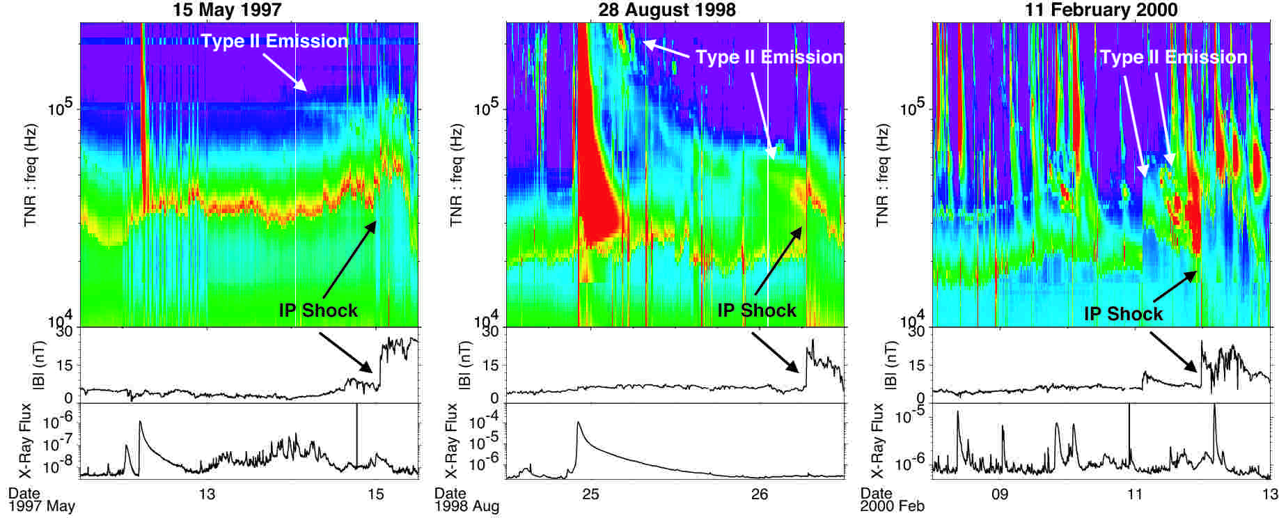
Figure 2: Radio wave, magnetic field, and GOES x-ray data for three shock crossings seen by the Wind spacecraft. The top panel is a dynamic spectrum from the WAVES instrument on Wind, the bottom panel is the x-ray flux data in the band $1-8\mbox{\AA}$ from the GOES-8 satellite (for May 1997) and the GOES-10 satellite (for August 1998 and February 2000.) The flare activity is shown by the x-ray peaks and type III radio bursts on 12 May 1997, 24 August 1998, and 9 February 2000. The type II emissions can be seen as slowly drifting features in the spectrum, and the spacecraft shock crossings are indicated by abrupt jumps in the local plasma frequency and the magnetic field.

Figure 2 shows dynamic spectra from Wind/WAVES and magnetic field data from the MFI instrument (Lepping et al., 1995) on Wind, along with GOES X-ray data for each of these three events. Upstream and downstream plasma parameters for each shock are listed in Table 2. At each event, the Wind spacecraft was in the foreshock region for a timespan of 20 to 40 seconds.

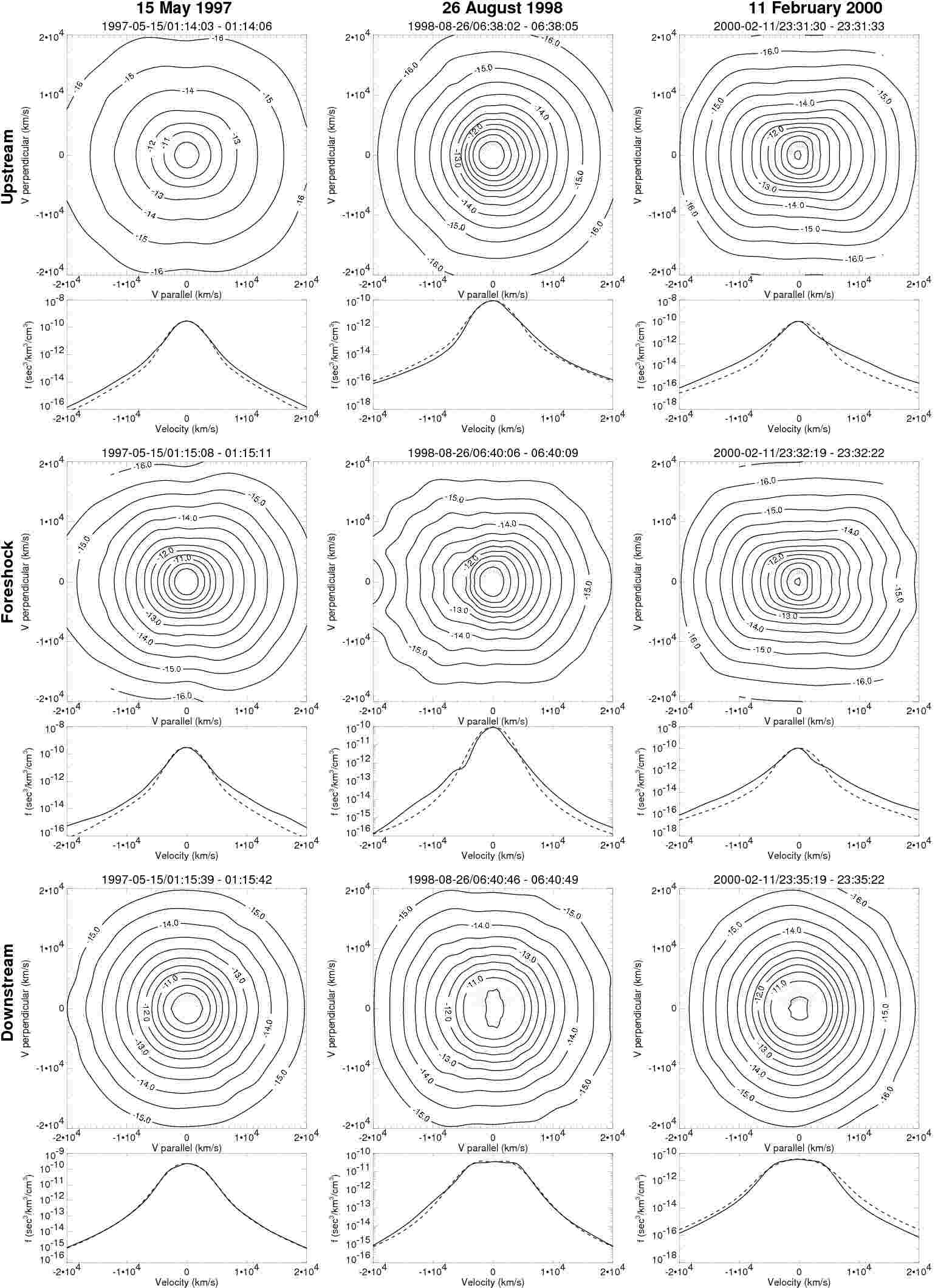
Figure 3: Electron velocity distributions measured by the EESA-L instrument on Wind during the upstream pre-foreshock, foreshock, and downstream periods for the three IP shocks. The foreshock region is characterized by bumps on the parallel distribution function and the loss cone evident in the 26 August 1998 and 11 February 2000 foreshock regions. The bottom part of each panel shows a parallel (solid line) and perpendicular (dashed line) cut through each two-dimensional distribution.

Figure 3 shows two-dimensional electron pitch angle distributions from the EESA-L instrument on Wind/3DP. The distributions are shown for each event in the upstream ‘pre-foreshock’ region, in the foreshock region, and in the downstream region after the shock has passed. The foreshock region is distinguished by the electron beams in the IMF-parallel direction, which can be seen as the bulges in the parallel and anti-parallel direction on the two-dimensional distributions and in the parallel (solid line) and perpendicular (dashed line) cuts. The observed electron distribution functions are consistent with the predictions of electron beams originating from the shock as predicted by Filbert & Kellogg (1979), and reflected by the Fast Fermi process described by Wu (1984) and Leroy & Mangeney (1984). The distribution functions also show an angular feature corresponding to a loss cone. This loss cone feature is predicted by the Fast Fermi theory and has been observed by Wind/3DP in the terrestrial foreshock. (Larson et al., 1996)

The electron beam reflected from the surface of the shock creates a bump on the tail of the electron distribution function. Due to velocity selection effects, this bump is most prominent at the boundary of the foreshock region. (Fitzenreiter et al., 1984) The Wind Solar Wind Experiment (SWE) (Ogilvie et al., 1995) has observed the positive slope at many encounters with the terrestrial foreshock boundary. (Fitzenreiter et al., 1996) However, the Wind/3DP instrument has insufficient energy resolution to resolve the positively sloped region on the tail of the distribution function, and therefore does not observe the bump during the same encounters.

After the arrival of the shock, the distributions display the broadened, flat-topped characteristics common to distributions downstream of strong interplanetary shocks. (Fitzenreiter et al., 2003)

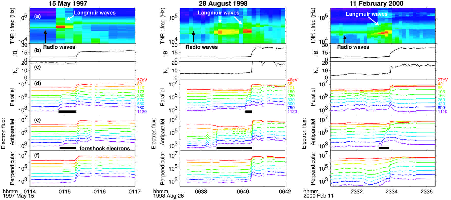
Figure 4: In situ particle and wave data from the Wind spacecraft for the three shock crossings. Panel (a) is a dynamic spectrum from the WAVES Thermal Noise Receiver, showing Langmuir wave activity in the foreshock region. Panels (b) and (c) are magnetic field and density measurements from MFI and 3DP, both showing a jump at the arrival of the shock. Panels (d), (e), and (f) are electron flux energy distributions from the EESA-L experiment on 3DP, in the parallel, antiparallel, and perpendicular directions. The foreshock electron beams are denoted by black bars in the parallel and antiparallel panels. The units for magnetic field are $\rm nT$, for density $\rm 1/cm^{3}$, and electron flux $\rm 1/eV/sec/cm^{2}/ster$.

The association of the foreshock electrons with the type II emission is established using the Langmuir wave observations from the WAVES instrument. Figure 4 shows wave and particle data from Wind at each shock crossing. Panel (a) is a WAVES dynamic spectrum showing intense Langmuir wave activity in each foreshock region. Panels (b) and (c) show magnetic field magnitude from MFI and proton density from 3DP. In both panels, there is a clear discontinuity as each shock crosses the spacecraft. The bottom three panels show electron energy flux for a range of energies measured by the low geometric factor Electron Electrostatic Analyzer (EESA-L) on 3DP. The Wind spacecraft was in burst mode during each shock crossing, measuring full three dimensional electron distributions once every three seconds. Panels (d), (e), and (f) show the IMF-parallel, antiparallel, and perpendicular fluxes, respectively. The Langmuir waves in panel (a) are associated with increases in electron flux in both the parallel and antiparallel directions, except for the 11 February 2000 shock, for which only antiparallel foreshock flux was observed. The black bars on the plots indicate the locations of elevated flux due to foreshock electrons. The correlation between foreshock electrons and Langmuir wave activity strongly indicates that these regions are sources of type II radio emission. In the following sections, we will use the electron burst data to characterize the shock-perpendicular scale height and shock-parallel scale distance of the foreshock region.

4 Shock-Perpendicular Scale Height

The scale height $d_{\perp}$ of the feature on the shock front is determined by the speed of the shock in the spacecraft frame $V_{sh}^{S/C}$ and the amount of time $\Delta t$ between the start of foreshock electron enhancement and arrival of the shock.

$$d_{\perp}\approx V_{sh}^{S/C}\cdot\Delta t$$ (1)

The time interval, indicated by the black bars in Figure 4, is easily measured. The shock velocity in the spacecraft frame is determined by mass flux conservation across the shock boundary (Paschmann & Schwartz, 2000), and is given by:

$$V_{sh}^{S/C}=\frac{\Delta(\rho\mathbf{V}^{S/C})}{\Delta{\rho}}\cdot\hat{\mathbf{n}}$$ (2)

where $\rho$ is the local mass density and $\hat{\mathbf{n}}$ is the unit vector normal to the shock surface. The determination of $\hat{\mathbf{n}}$ is discussed in a later section.

The scale height of the 26 August 1998 shock was calculated in Bale et al. (1999) and found to be $136,000\>\mathrm{km}\>(21.3\>R_{E})$ for $d_{-\perp}$, the height of the structure in the antiparallel direction, and $25,000\>\mathrm{km}\>(3.9\>R_{E})$ for $d_{\perp}$, in the parallel direction. Our method yields the significantly smaller values of $69,000\>\mathrm{km}\>(10.1\>R_{E})$ for $d_{-\perp}$ and $15,000\>\mathrm{km}\>(3.9\>R_{E})$ for $d_{\perp}$. These results differ because Bale et al. (1999) uses the total time between the start of the flare and arrival of the shock to calculate an average shock speed from the inner heliosphere to 1 AU. Here we use the in situ method described above, which yields an instantaneous $V_{sh}$ that more accurately describes the local shock parameters.

The calculated values of $d_{\perp}$ and $d_{-\perp}$ for each of the three analyzed shocks are listed in Table 3.

5 Estimating Shock-Parallel Distance

When electrons reflect from the shock surface and stream along IMF lines to the spacecraft, the most energetic accelerated electrons will arrive first, followed by the lower energy electrons. Provided that the distance from the acceleration point is sufficiently large and the energy and time resolution of the detector is sufficiently good, this time of flight dispersion is observable in the foreshock electron beam.

The velocity of the electrons is determined by the (nonrelativistic) formula

$$v_{e}=\sqrt{2E/m_{e}}$$ (3)

where E is the kinetic energy of the electron.

We assume that the electrons were accelerated instantaneously at a time $t_{0}$. The transit time for each energy bin is determined by the time interval between $t_{0}$ and $t_{onset}$, when the first enhancement appeared in that bin. The parallel distance $d_{\parallel}$ and the initial acceleration time $t_{0}$ are determined by fitting the measured values of $v_{e}$ and $t_{onset}$ to the simple functional form

$$d_{\parallel}=v_{e}(t_{onset}-t_{0})=v_{e}\cdot\Delta t$$ (4)

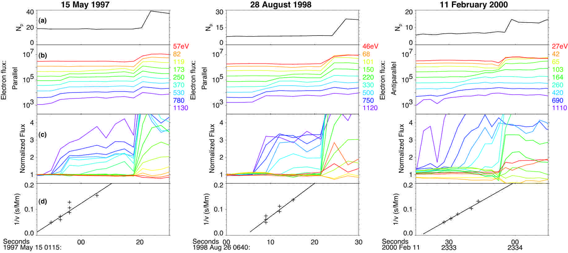
Figure 5: In situ particle data from the Wind 3DP instrument. Panel (a) is the particle density, showing the shock arrival time. Panel (b) is the parallel (antiparallel for 11 February 2000) electron energy distribution, showing the velocity dispersed electron beam. Panel (c) emphasizes the velocity dispersion by normalizing each energy channel to its pre-foreshock flux. Panel (d) shows a fit of arrival time to inverse electron velocity, as described in Equation 4.

The results of this fit are shown in Figure 5, which contains in situ data from the Wind/3DP in the foreshock region, for each of the three analyzed shocks. For each shock, only one of two possible directions contained sufficient velocity dispersion in the electron beam that the above equation could be fit. For the 15 May 1997 and 28 August 1998 shock, the parallel direction was fit. For the 11 February 2000 shock, the antiparallel direction was fit.

The proton density is plotted in panel (a). The jump in density indicates arrival of the shock. Panel (b) shows the flux of electrons parallel (or antiparallel for 11 February 2000) to $\mathbf{B}$ prior to shock arrival. Note that flux enhancement occurs first in the high energy electron bins. Panel (c) shows the same electron flux, with each energy bin normalized to its preshock level. The onset time for each energy bin is defined as the time when the normalized flux first rises past a threshold value. Panel (d) shows a fit of onset time against inverse velocity for each energy bin which showed foreshock enhancement. $t_{acc}$ and $d_{\parallel}$ are given by fitting the velocity and time data to Equation 4.

It is important to clarify the relationship between Equation 4 and the ‘foreshock coordinate system’ established by Filbert & Kellogg (1979). Filbert & Kellogg (1979) noted that velocity-dispersed electrons will be a steady-state spatial feature of an electron foreshock in the shock frame. A ‘cutoff’ velocity $v_{c}$ exists below which the shock-accelerated electrons will not reach the spacecraft; the result is a beam-like feature that is unstable to Langmuir waves. Filbert & Kellogg (1979) showed that $v_{c}\approx v_{sw}d_{\parallel}/DIFF$, where $DIFF$ is the distance downstream from the first tangent field line to the shock, in the direction of the solar wind flow. In our formulation, $DIFF=v_{sh}\Delta t\approx v_{sw}\Delta t$ so that $d_{\parallel}=v_{c}\Delta t$, which is equivalent to Equation 4. Hence this is just a transformation from the shock frame to the spacecraft frame.

For the 26 August 1998 shock discussed in Bale et al. (1999), the fit value for the shock parallel distance $d_{\parallel}$ is $78,000\>\mathrm{km}\>(12.2\>R_{E})$. The parallel beam for the 15 May 1997 shock and the antiparallel beam for the 11 February 2000 shock were also fit using this method, yielding $d_{\parallel}=136,000\>\mathrm{km}\>(21.2\>R_{E})$ for the 15 May 1997 shock and $d_{-\parallel}=151,000\>\mathrm{km}\>(32.6\>R_{E})$ for the 11 February 2000 shock.

The antiparallel foreshock beams seen in the 15 May 1997 and 26 August 1998 shocks do not display velocity dispersed onset times, implying that the acceleration site was close to the spacecraft. An upper limit on $d_{-\parallel}$ may be obtained by noting that if the fastest and slowest foreshock electrons arrived at the spacecraft at the same time to within the time resolution of 3DP burst mode, then $d_{-\parallel}$ must satisfy

$$d_{-\parallel}/v_{slow}-d_{-\parallel}/v_{fast}\leq 3~{}\mathrm{seconds}$$ (5)

which yields an upper limit for $d_{-\parallel}\leq 140,000\>\mathrm{km}\>(21.9\>R_{E})$ for 15 May 1997 and $d_{-\parallel}\leq 26,000\>\mathrm{km}\>(4.0\>R_{E})$ for 28 August 1998.

The calculated values of $d_{\parallel}$ and $d_{-\parallel}$ for all of the analyzed shocks are listed in Table 3.

6 Upstream IMF and coplanarity of shock front

In our calculation of $d_{\parallel}$ and $d_{\perp}$, we have made two assumptions about the magnetic field: that the IMF line connecting the shock to the spacecraft is straight, and that the shock propagation direction is perpendicular to the IMF lines. In this section, we investigate the validity of these assumptions.

The boundary of the electron foreshock region is determined by the IMF line tangent to the shock surface. Turbulence in the solar wind and electromagnetic radiation generated by shock-accelerated particles can deform the structure of the IMF. Numerical models of magnetic field line transport have been developed to simulate IMF conditions at planetary bow shocks. (Zimbardo & Veltri, 1996)

For IMF conditions similar to those at 1 AU, the ratio of the spread in the foreshock boundary $\Delta r$ to the length of the connecting IMF line $r$ is $\Delta r/r\approx 0.1$. If $\Delta r/r>d_{\perp}/d_{\parallel}$, then the foreshock measurements could be explained simply as an effect of turbulence in the IMF. However, for each analyzed shock, $d_{\perp}/d_{\parallel}$ (and $d_{-\perp}/d_{-\parallel}$) is greater than $0.1$, so magnetic turbulence alone cannot account for the apparent structure on the shock front.

If the IMF lines are straight, but the shock front is not coplanar with the IMF lines, then the time of flight dispersion analysis can yield misleading results for the perpendicular distance to the shock. The above analysis assumes a coplanar structure, so we must establish that this is a good approximation.

The orientation of the shock to the IMF can be determined by mixed mode (including both field and particle data) coplanarity analysis. The coplanarity theorem for compressive shocks states that the shock normal ($\mathbf{\hat{n}}$), the upstream and downstream magnetic fields ($\mathbf{B}_{u}$ and $\mathbf{B}_{d}$), and the velocity jump across the shock ($\Delta\mathbf{V}$) all lie in the same plane. If $\Delta\mathbf{B}\equiv\mathbf{B}_{d}-\mathbf{B}_{u}$ is the change in magnetic field, then the shock normal (Paschmann & Schwartz, 2000) is given by:

$${\mathbf{\hat{n}}=\frac{(\Delta\mathbf{B}\times\Delta\mathbf{V})\times\Delta\mathbf{B}}{|(\Delta\mathbf{B}\times\Delta\mathbf{V})\times\Delta\mathbf{B}|}}$$ (6)

The perpendicularity of the shock is measured by $\theta_{bn}$, the angle between the upstream magnetic field $\mathbf{B}_{u}$ and $\mathbf{\hat{n}}$. To check consistency, we also calculate $\theta_{bn}$ using $\mathbf{B}_{u}$ and $\mathbf{B}_{d}$ in place of $\Delta\mathbf{B}$ in Equation 6. (Paschmann & Schwartz, 2000) Values for $\theta_{bn}$ for each shock are listed in Table 2.

For each mixed mode calculation at each shock, $\theta_{bn}>80^{\circ}$, so the assumption of a locally perpendicular shock front at Wind is a good one, and the angle between the shock front and magnetic field does not introduce large errors in our calculation of $d_{\parallel}$ or $d_{\perp}$.

7 Discussion

We have conducted a survey of several hundred IP shocks, and found in situ type II radiation, correlated with IMF-parallel electron beams, present at eight IP shocks. Most IP shocks do not show evidence of in situ type II radiation, and of those that do, few show evidence of upstream electron beams observable by the Wind spacecraft. However, this does not disprove the IP foreshock mechanism as the generator of type II radiation. The proposed mechanism is a localized phenomenon, while the consequent radiation is visible throughout the heliosphere. It is quite unlikely that any given region of localized emission will be encountered by the Wind spacecraft. The exact probability of such an encounter depends on the size and number of IP foreshock regions, and this paper represents a first attempt at quantifying both. Of the events which do present observed in situ type II radiation, the low number of events with correlated waves and electron beams is primarily due to the infrequent availability of high cadence measurements of the electron distributions.

In addition to the survey of the Wind data set, we present detailed in situ observations of the electron foreshock region of three IP shocks. In each of these three events, the presence of velocity dispersion in the foreshock electron measurements allows calculation of the parallel and perpendicular scale size of shock front structure. The 15 May 1997 and 28 August 1998 shocks have evidence for foreshock structure in both the parallel and antiparallel directions, suggesting the presence of a bay in which electron beams can be mirrored and accelerated, generating Langmuir waves and radio emission.

Although foreshock regions upstream of IP shocks imply curved structures, the foreshock regions could theoretically be created by either a curved magnetic field or by a curved shock. Using only measurements made by a single spacecraft, it is impossible to determine which effect predominates. Previous studies focused on ion acceleration have assumed both cases: propagation of a planar shock through a region of curved magnetic fields (Erdos & Balogh, 1994), or ion acceleration by repeated encounters with a rippled shock. (Decker, 1990) It is shown in the previous section that upstream magnetic turbulence alone cannot explain the dimensions of the acceleration regions, and therefore at least a portion of the foreshock region must be created by shock front structure. Regardless of which effect predominates, the methodology used in this paper to estimate the characteristic dimensions of the foreshock regions is valid.

It is unclear at present what causes the observed shock front structure. The curvature may be caused by Alfvén speed inhomogeneities in the solar wind, which can allow different sections of the shock to propagate at different speeds through the heliosphere. Shock reformation, a process in which protons reflected from a shock surface generate upstream instabilities which lead to formation of a new shock front upstream of the original front, may also play a role. One-dimensional hybrid simulations suggest that shock reformation in perpendicular shocks depends on upstream parameters such as Mach number and plasma $\beta$. (Hellinger et al., 2002) However, more recent two-dimensional studies suggest that perpendicular shock fronts may be dominated by whistler waves, which can inhibit reformation. (Hellinger et al., 2007)

Multi-spacecraft missions such as STEREO will be greatly helpful in future investigations of shock structure, and future studies with multi-point measurements should improve current estimates of the frequency and size of IP foreshock regions, which will provide useful input for models of type II generation. If shock front structure is a common feature of IP shocks, then each foreshock region on a shock front would create an independent source of type II radio emission. The spatial variation in upstream plasma density at these multiple source regions could then be responsible for the fine structure observed in many type II bursts.

Table 1: IP Shocks With Observed in situ Type II Source Regions

LASCO CME			IP Shock			Burst	Velocity	Type II
Year	Date	Time	Year	Date	Time	Data	Dispersion	Emission
1997	May 12	0530	1997	May 15	0115	X	X	X
1998	Aug 24	2209	1998	Aug 26	0640	X	X	X
2000	Feb 10	0230	2000	Feb 11	2333	X	X	X
2000	Feb 17	0431	2000	Feb 20	2045	X		X
2000	Oct 02	0350	2000	Oct 05	0240	X
2000	Oct 09	2350	2000	Oct 12	2145	X
2001	Mar 19	0526	2001	Mar 22	1355
2001	Dec 26	0530	2001	Dec 30	2005	X		X

Table 2: Shock and Plasma Parameters for Selected Events

Date	$\mathrm{UT}$	$\mathrm{B_{1}/B_{0}}$	$V_{sh}^{S/C}\>(\mathrm{km/s})$	$\mathrm{U_{sw}\>(km/s)}$	$\mathrm{M_{A}}$	$\beta$	$r_{L}\>(\mathrm{km})$	$\theta_{bn}$
15 May 1997	0115	2.19	423.	321.	2.62	0.44	392.	89.9
26 August 1998	0640	3.09	659.	493.	2.63	0.66	665.	88.1
11 February 2000	2333	3.24	678.	458.	3.19	0.39	654.	85.7

Table 3: Shock Structure Parameters ($d$ measured in Mm ($R_{E}$))

Date	$t_{0}$	$t_{shock}$	$d_{\perp}$		$d_{\parallel}$		$d_{-\perp}$		$d_{-\parallel}$
15 May 1997	01:14:43	01:15:23	17	(2.6)	136	(21.2)	17	(2.6)	$\leq 140$	(21.9)
26 August 1998	06:40:04	06:40:27	15	(2.3)	78	(12.2)	69	(10.1)	$\leq 26$	(4.0)
11 February 2000	23:32:55	23:33:58	$\cdots$	$\cdots$	$\cdots$	$\cdots$	28	(4.3)	151	(32.6)

Figure 1: A cartoon of shock structure consistent with our observations. Electron flux in the $\mathbf{B}$ and $-\mathbf{B}$ direction increases previous to shock arrival, as Wind is connected along the IMF line to an advanced section of the shock front. Langmuir waves and electron beams are observed in the foreshock region.

References

- Anderson et al. (1979) Anderson, K. A., Lin, R. P., Martel, F., Lin, C. S., Parks, G. K., & Reme, H. 1979, Geophys. Res. Lett., 6, 401
- Bale et al. (1999) Bale, S. D., Reiner, M. J., Bougeret, J.-L., Kaiser, M. L., Krucker, S., Larson, D. E., & Lin, R. P. 1999, Geophys. Res. Lett., 26, 1573
- Bougeret et al. (1995) Bougeret, J.-L., Kaiser, M. L., Kellogg, P. J., Manning, R., Goetz, K., Monson, S. J., Monge, N., Friel, L., Meetre, C. A., Perche, C., Sitruk, L., & Hoang, S. 1995, Space Science Reviews, 71, 231
- Cairns (1986) Cairns, I. H. 1986, Proceedings of the Astronomical Society of Australia, 6, 444
- Cairns et al. (2003) Cairns, I. H., Knock, S. A., Robinson, P. A., & Kuncic, Z. 2003, Space Science Reviews, 107, 27
- Cane & Richardson (2003) Cane, H. V. & Richardson, I. G. 2003, Journal of Geophysical Research (Space Physics), 108, 6
- Decker (1990) Decker, R. B. 1990, J. Geophys. Res., 95, 11993
- Erdos & Balogh (1994) Erdos, G. & Balogh, A. 1994, ApJS, 90, 553
- Filbert & Kellogg (1979) Filbert, P. C. & Kellogg, P. J. 1979, J. Geophys. Res., 84, 1369
- Fitzenreiter et al. (1984) Fitzenreiter, R. J., Klimas, A. J., & Scudder, J. D. 1984, Geophys. Res. Lett., 11, 496
- Fitzenreiter et al. (2003) Fitzenreiter, R. J., Ogilvie, K. W., Bale, S. D., & Viñas, A. F. 2003, Journal of Geophysical Research (Space Physics), 108, 1
- Fitzenreiter et al. (1996) Fitzenreiter, R. J., Viňas, A. F., Klimas, A. J., Lepping, R. P., Kaiser, M. L., & Onsager, T. G. 1996, Geophys. Res. Lett., 23, 1235
- Hellinger et al. (2002) Hellinger, P., Trávnícek, P., & Matsumoto, H. 2002, Geophys. Res. Lett., 29, 87
- Hellinger et al. (2007) Hellinger, P., Trávníček, P., Lembège, B., & Savoini, P. 2007, Geophys. Res. Lett., 34, 14109
- Knock et al. (2001) Knock, S. A., Cairns, I. H., Robinson, P. A., & Kuncic, Z. 2001, J. Geophys. Res., 106, 25041
- Knock et al. (2003) —. 2003, Journal of Geophysical Research (Space Physics), 108, 6
- Krauss-Varban & Burgess (1991) Krauss-Varban, D. & Burgess, D. 1991, J. Geophys. Res., 96, 143
- Krauss-Varban et al. (1989) Krauss-Varban, D., Burgess, D., & Wu, C. S. 1989, J. Geophys. Res., 94, 15089
- Larson et al. (1996) Larson, D. E., Lin, R. P., McFadden, J. P., Ergun, R. E., Carlson, C. W., Anderson, K. A., Phan, T. D., McCarthy, M. P., Parks, G. K., Rème, H., Bosqued, J. M., d’Uston, C., Sanderson, T. R., Wenzel, K.-P., & Lepping, R. P. 1996, Geophys. Res. Lett., 23, 2203
- Lepping et al. (1995) Lepping, R. P., Acuna, M. H., Burlaga, L. F., Farrell, W. M., Slavin, J. A., Schatten, K. H., Mariani, F., Ness, N. F., Neubauer, F. M., Whang, Y. C., Byrnes, J. B., Kennon, R. S., Panetta, P. V., Scheifele, J., & Worley, E. M. 1995, Space Science Reviews, 71, 207
- Leroy & Mangeney (1984) Leroy, M. M. & Mangeney, A. 1984, Annales Geophysicae, 2, 449
- Lin et al. (1995) Lin, R. P., Anderson, K. A., Ashford, S., Carlson, C., Curtis, D., Ergun, R., Larson, D., McFadden, J., McCarthy, M., Parks, G. K., Reme, H., Bosqued, J. M., Coutelier, J., Cotin, F., D’Uston, C., Wenzel, K.-P., Sanderson, T. R., Henrion, J., Ronnet, J. C., & Paschmann, G. 1995, Space Science Reviews, 71, 125
- Manoharan et al. (2004) Manoharan, P. K., Gopalswamy, N., Yashiro, S., Lara, A., Michalek, G., & Howard, R. A. 2004, Journal of Geophysical Research (Space Physics), 109, 6109
- Ogilvie et al. (1995) Ogilvie, K. W., Chornay, D. J., Fritzenreiter, R. J., Hunsaker, F., Keller, J., Lobell, J., Miller, G., Scudder, J. D., Sittler, Jr., E. C., Torbert, R. B., Bodet, D., Needell, G., Lazarus, A. J., Steinberg, J. T., Tappan, J. H., Mavretic, A., & Gergin, E. 1995, Space Science Reviews, 71, 55
- Paschmann & Schwartz (2000) Paschmann, G. & Schwartz, S. J. 2000, in ESA Special Publication, Vol. 449, Cluster-II Workshop Multiscale / Multipoint Plasma Measurements, ed. R. A. Harris, 99–+
- Reiner et al. (1998a) Reiner, M. J., Kaiser, M. L., Fainberg, J., Bougeret, J.-L., & Stone, R. G. 1998a, Geophys. Res. Lett., 25, 2493
- Reiner et al. (1998b) Reiner, M. J., Kaiser, M. L., Fainberg, J., & Stone, R. G. 1998b, J. Geophys. Res., 103, 29651
- Wu (1984) Wu, C. S. 1984, J. Geophys. Res., 89, 8857
- Zimbardo & Veltri (1996) Zimbardo, G. & Veltri, P. 1996, Geophys. Res. Lett., 23, 793