Average Density of States in Disordered Graphene systems

Abstract

In this paper, the average density of states (ADOS) with a binary alloy disorder in disordered graphene systems are calculated based on the recursion method. We observe an obvious resonant peak caused by interactions with surrounding impurities and an anti-resonance dip in ADOS curves near the Dirac point. We also find that the resonance energy ($E_{r}$) and the dip position ($\varepsilon_{dip}$) are sensitive to the concentration of disorders ($x$) and their on-site potentials ($v$). An linear relation, $\varepsilon_{dip}$=$xv$, not only holds when the impurity concentration is low but this relation can be further extended to high impurity concentration regime with certain constraints. We also calculate the ADOS with a finite density of vacancies and compare our results with the previous theoretical results.

I Introduction

Graphene is a two-dimensional (2D) material with a single atomic layer of graphite. The material has been fabricated firstly by rubbing graphite layers against an oxidized silicon surface recently.Science06-Nov Due to the linear dispersion relation of its electronic spectrum near the Dirac point, the electron transport behavior of graphene at low energy range is essentially determined by the massless relativistic Dirac’s equations. Many interesting properties of graphene have been studied experimentally and theoretically by many research groups, including the unusual quantum Hall effect,Nature05-Nov ; Nature05-Zha ; Cond-mat05-Per ; PRB06-Per quantum minimal conductivity,PRB06-Per ; EPJ06-Kat ; PRB07-Cse ; PRL07-Zie ; PRB06-Gus ; PRB07-Zie ; PRL07-Ken ferromagnetism,AdvMater03-Han ; PRB05-Voz and superconductivity.PRB97-Tam ; JSoc97-Nak ; JLowTemp00-Kop

The disorder in graphenes can significantly impact their electronic properties and has been studied extensively.J.Mol.Str.91-Ovc ; PRL92-Gon ; PRB96-Cha ; PRL00-Wak ; PRB01-Wak ; PRB01-Gon ; JPCM01-Har ; JPSJ01-Mat ; JPCS04-Har ; PRL04-Dup ; PRL04-Leh ; PRB05-Voz It is believed that the interplay between disorders and electron-electron interactions determine the low energy behavior of the electron in the graphene system. Due to disorders, the average density states (ADOS) increases at the Dirac points.PRB06-Per The ADOS is actually an important parameter to describe electronic structures, especially in a disordered system. The minimum conductivity ($\sigma_{min}$), for instance, can be obtained by calculating the diffusion constant ($D$) and ADOS ($\rho$) at the Fermi level through the Einstein relation ($\sigma_{min}=\rho D$). To date, various methods have been proposed to calculate ADOS and the local density of states (LDOS) in various types of disordered graphenes, such as Anderson disorder,PRB84-Hu short-range potential disorder,PRL07-Ken ; PRB06-Skr ; PRB07-Skr ; PRB07-Weh ; Cond-mat06-Pog , long-range potential disorderPRL07-Ken , and vacancy.PRB06-Per ; PRL06-Pere ; Cond-mat05-Per However, these calculation results are unreliable due to the limitations of approximation, or these calculations are only suitable to address electronic structure with a low impurity concentration. It is, therefore, important to obtain the accurate electronic structures of disordered graphenes.

Recently, the phenomenon of spectrum rearrangement has been studied in a binary alloy disorder in disordered graphene. Due to the limitation of the coherence potential approximation (CPA),PRB07-Skr ; PRB04-Skr the corresponding results are appropriate to address the electronic structures of graphene with an extreme low impurity concentration. In this paper, we calculate the ADOS with the similar system by using the recursion method. Our numerical simulations provide the accurate ADOS for different impurity concentrations. Moreover, our simulation can also be generalized to study other types of disordered graphene. Though the main features of ADOS with a binary alloy disorder in graphene can be described using the resonant and anti-resonant states caused by scattering of a impurity as reported in Ref. 20. Interestingly, we observe that the impurity concentration ($x$) and the on-site potential ($v$) have significant impact on the main features of ADOS. The impurity concentration shifts the position of resonance energy ($E_{r}$). An linear relation for the anti-resonance dip shift ($\varepsilon_{dip}=xv$) with a relative low impurity concentration can be extended to a high impurity concentration case under certain conditions. Moreover, the ADOS with a finite concentration of vacancies is also calculated using our proposed approach and compared with the other previous theoretical results.

This paper is organized as follows. The tight-binding model of graphene with a binary alloy disorder is given in Sec. II A. The recursion method is introduced and its accuracy and applications are explored in Sec. II B. The ADOS of graphene with different impurity concentrations and on-site potentials are calculated and the detailed discussions are given in Sec. III. Finally, we conclude our contributions in Sec. IV.

II Computational Model and Method

II.1 Model

Fig. 1 shows the hexagonal lattice structure of a graphene and each unit cell has two inequivalent atoms labeled A and B, respectively. If we consider the contribution from the $\pi$ bond (one $\pi$ electron per atom) and the nearest interactions in the graphene, the Hamiltonian based on the Wannier representation can be expressed as

$$\hat{H}=\sum_{i}\varepsilon_{i}|i\rangle\langle i|-t_{ij}\sum_{\langle i,j\rangle}|i\rangle\langle j|,$$ (1)

where, i and j denote the neighboring sites on the lattice, $\varepsilon_{i}$ is the on-site energy, and $t_{ij}$ is the nearest hopping energy ($t_{ij}$=$t$ and its value is close to 2.7 eV in graphenes). For simplicity, here $t$ is scaled to be 1.

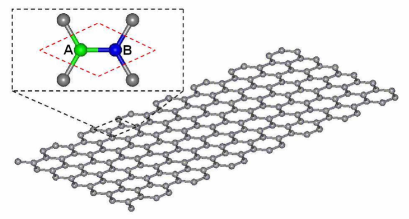
Figure 1: (Color online) A honeycomb lattice of a graphene. Here, an unit cell is outlined by the red dashed lines. Two inequivalent atoms in the unit cell are labeled with A (the green sphere) and $B$ (the blue one), respectively.

With a given impurity concentration ($x$), the on-site energy $\varepsilon_{i}$ for a binary alloy disordered system equals $v$ with probability $x$, or zero otherwise. This model, which is attributed to Lifshiz,Adv. Phys.64-Lif , features the absolutely random distribution of impurities in the space domain. In our following calculations, we emphasize on studying the properties of the ADOS in two cases. One is on-site potential ($v$) varies with given disorder concentrations ($x$). In the other case, the concentration ($x$) changes with given on-site potentials ($v$).

II.2 The Recursion Method

The Lanczos methodJRNAB50-Lan (so called the Haydock-Heine-Kelly recursion methodJPC72-Hay ; JPC75-Hay ) is a commonly used approaches to calculate the ADOS in disorder systems. The essential idea of the recursion method is that the Hamiltonian matrix is expressed using a tridiagonal representation iteratively. After selecting a localized seed-state ($|f_{0}\rangle$), this recursion method generates a hierarchy of states ($|f_{n}\rangle$) based on a defined orthogonal basis recursively.

$$|f_{n+1}\rangle=\hat{H}|f_{n+1}\rangle-\frac{\langle f_{n}|\hat{H}|f_{n}\rangle}{\langle f_{n}|f_{n}\rangle}|f_{n}\rangle-\frac{\langle f_{n}|f_{n}\rangle}{\langle f_{n-1}|f_{n-1}\rangle}|f_{n-1}\rangle,$$ (2)

where, $n=0,1,2,\cdots$, and the recursive coefficients are given by

$$a_{n}=\frac{\langle f_{n}|\hat{H}|f_{n}\rangle}{\langle f_{n}|f_{n}\rangle},b_{n}=\frac{\langle f_{n}|f_{n}\rangle}{\langle f_{n-1}|f_{n-1}\rangle}(b_{0}=0,|f_{-1}\rangle=0).$$ (3)

In the orthogonal basis, the Hamilton matrix becomes

$$H=\begin{pmatrix}a_{0}&b_{1}&0&0&\cdots\\ b_{1}&a_{1}&b_{2}&0&\cdots\\ 0&b_{2}&a_{2}&b_{3}&\cdots\\ 0&0&b_{3}&a_{3}&\cdots\\ \vdots&\vdots&\vdots&\vdots&\ddots.\end{pmatrix}$$ (4)

The diagonal elements in a Green’s function matrix for a seed state can be derived from Eq. (4) based on the continuous-fraction method.

$$G_{00}(E) = \langle f_{0}|\cfrac{1}{E-H}|f_{0}\rangle$$ (5)

$$= \cfrac{1}{E-a_{0}-\cfrac{b_{1}^{2}}{E-a_{1}-\cfrac{b_{2}^{2}}{E-a_{2}-\cfrac{b_{3}^{2}}{\ddots}}}}$$

and LDOS is defined as

$$\rho_{local}(E)=\lim\limits_{\varepsilon\to 0^{+}}[-\frac{1}{\pi}G_{00}(E+i\varepsilon)].$$ (6)

We can then calculate ADOS easily using the following equation

$$\rho_{aver}(E)=\frac{1}{M}\sum_{M}\rho_{local}(E),$$ (7)

where $M$ is the number of the samples. To terminate continuous fractions, Eq. (5) can be rewritten as

$$G_{00}(E)=\cfrac{1}{E-a_{0}-\cfrac{b_{1}^{2}}{E-a_{1}-\cfrac{b_{2}^{2}}{\cfrac{\cdots}{E-a_{n}-t(E)}}}}.$$ (8)

In above equation, the terminating term can be written as

$$t(E)=\cfrac{1}{2}\{(E-a_{\infty})-[(E-a_{\infty})^{2}-4b_{\infty}^{2}]\}.$$ (9)

The asymptotic value of the continuous-fraction coefficient pairs $(a_{\infty},b_{\infty})$ in above equation can be obtained when $n$ gets large.

This recursion method has been adopted to investigate various disorder systems.PRB94-Hay ; PRB82-Sin ; PRB89-Loh In fact, an infinite system can be approximated with periodic boundary condition using this method and the numerical error of DOS is easy to estimate.PRB94-Hay If the system size ($L$) and its recursion step ($N$) are large enough and corresponding positive broadening width ($\varepsilon$) is reasonably small, the LDOS results should be accurate. It is easy to get a reliable ADOS of a disorder system by averaging over a large number of samples ($M$). For a perfect graphene, two relations, $\varepsilon\sim 1/L$ and $\rho\sim 1/L$, hold approximately at the Dirac point as shown in Figs. 2 $(a)$ and $(b)$, respectively. The results suggest that the DOS in a large finite system is close to that in an infinite system. Of course, to obtain a reliable ADOS result, a large recursion step $N$ is needed, which should be larger than $L$, i.e. 2$L$ [Fig. 2$(c)$].

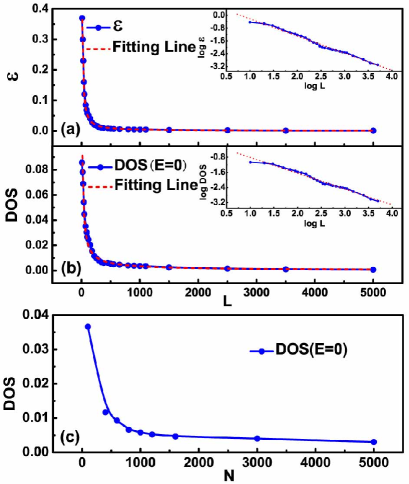
Figure 2: (Color online) (a) $\varepsilon$ as a function of $L$ (the blue solid line) and the corresponding fitting line shown with red dashed line for a perfect graphene. (b) DOS ($\rho$) as a function of $L$ (the blue solid line) and corresponding fitting line with the red dashed line. (c) DOS ($\rho$) as a function of $N$ (the blue solid line) at the Dirac point ($E=0$). Here, $L=800$.

The accuracy of the recursion method is examined by comparing the calculated DOS of a perfect graphene with those obtained based on the strict integral method in the first Brillouin zone. The calculated DOS at several energy points are list in Table I. Clearly, the results using the recursion method are reliable and their relative errors are very small. In what follows, we calculate the ADOS of a disorder graphene and the parameters, $L=800$, $N=2L$, $\varepsilon=5\times 10^{-3}$ and $M=1000$, are chosen.

Table 1: The calculated density of state in a perfect graphene using both the recursion method and the strict integral method within the first BZ. Here, $L=800$, $N=2L$ and $\varepsilon=5\times 10^{-3}$.

Energy	$0.0$	$0.4$	$0.8$	$1.2$	$1.6$	$2.0$
REM	$0.0037$	$0.0781$	$0.1990$	$0.2570$	$0.1952$	$0.1702$
INM	$0.0037$	$0.0781$	$0.1998$	$0.2529$	$0.1938$	$0.1695$
Error	$<0.0001$	$<0.0001$	$<0.002$	$<0.002$	$<0.002$	$<0.002$

III Results and Discussion

Fig. 3(a) shows several calculated ADOS of graphene with the fixed impurity concentration $x=10\%$, but different on-site potentials ($v$). Our results clearly show that ADOS remains the similar shape in a high energy region. However, the ADOS near the Dirac point changes remarkably for different on-site potential ($v$). Two obvious features are observed. (1) An obvious resonance peak appears in the ADOS curves when $v\geq 3$. Its energy position or the resonance energy ($E_{r}$) shifts towards the Dirac point when the on-site potential ($v$) increases. This peak is attributed to a resonance state. A very similar feature was also observed in the LDOS when there is a single impurity or a low impurity concentration.PRB06-Skr ; PRB07-Skr (2) There is a dip near the Dirac point, which results from an antiresonance state. The position of this anti-resonance dip ($\varepsilon_{dip}$) shifts due to the presence of impurities. As shown in Fig. 3(b), the linear relation, $\varepsilon_{dip}$=$xv$, holds when the on-site potential is relatively small, but the dip disappears when $v$ becomes larger $(i.e.v>3)$. These results show that the relation ($\varepsilon_{dip}$=$xv$) is correct when $v\ll v_{dip}$, while this relation does not hold for a system with on-site potential $v>v_{dip}$.

To quantitatively explore the impurity concentration how to shift the position of resonance energy ($E_{r}$), we compare the result for the finite concentration with that for a single impurity. The calculated results are shown in Fig. 3(c). Here, we adopted the recursion method and the effective-mass approximation method (EMA)PRB06-Wang to determined the position of resonance energy ($E_{r}$) of LDOS at impurity site for a single impurity in the graphene system respectively. We also calculate resonance energy ($E_{r}$) of ADOS for the finite impurity concentration by using the recursion method.

The Green’s function in a perfect graphene based on the effective-mass approximation is expressed as

$$G_{0}(E) = \lim\limits_{\varepsilon\to 0^{+}}\cfrac{S}{\pi}\int_{0}^{k_{c}}\cfrac{(E+i\varepsilon)k}{(E+i\varepsilon)^{2}+(3tak/2)^{2}}dk$$ (10)

$$= \cfrac{\sqrt{3}}{3\pi t^{2}}E\ln|\cfrac{E^{2}}{9t^{2}a^{2}k_{c}^{2}/4-E^{2}}|-i\cfrac{\sqrt{3}}{3t^{2}}|E|$$

$$= \cfrac{\sqrt{3}}{3\pi}E\ln|\cfrac{E^{2}}{9a^{2}k_{c}^{2}/4-E^{2}}|-i\cfrac{\sqrt{3}}{3}|E|,$$

where $S=3\sqrt{3}a^{2}/2$ is the area of a unit cell in real space. $a$ is lattice constant. $k_{c}$ is cutoff wave vector and is set to be $2.13/a$.PRB06-Wang For a simple case, the Green’s function of a single impurity graphene is expressed as

$$G(E) = \cfrac{G_{0}(E)}{1-vG_{0}(E)}=(\cfrac{\sqrt{3}}{3\pi}E\ln|\cfrac{E^{2}}{9a^{2}k_{c}^{2}/4-E^{2}}|$$ (11)

$$-\cfrac{v}{3\pi}E^{2}\ln^{2}|\cfrac{E^{2}}{9a^{2}k_{c}^{2}4-E^{2}}|-\cfrac{v^{2}}{3}E^{2}-i\cfrac{\sqrt{3}}{3}|E|)$$

$$/([1-\cfrac{\sqrt{3}}{3\pi}E\ln|\cfrac{E^{2}}{9a^{2}k_{c}^{2}/4-E^{2}}|]^{2}+\cfrac{v^{2}}{3}E^{2}).$$

LDOS at the impurity site is easy to obtain by

$$\rho_{imp}(E)=\cfrac{\sqrt{3}}{3\pi}\cfrac{|E|}{[1-\cfrac{\sqrt{3}}{3\pi}E\ln|\cfrac{E^{2}}{9a^{2}k_{c}^{2}/4-E^{2}}|]^{2}+\cfrac{v^{2}}{3}E^{2}}.$$ (12)

The resonant energy ($E_{r}$) in this case can be defined using the Lifshits equation as

$$1=vReG_{0}(E_{r})=\cfrac{\sqrt{3}v}{3\pi}E_{r}\ln|\cfrac{E^{2}_{r}}{9a^{2}k_{c}^{2}/4-E^{2}_{r}}|.$$ (13)

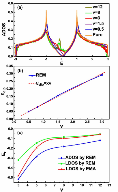
Figure 3: (Color online) (a) ADOS ($\rho$) of a graphene with impurity concentration $x=10\%$ and various on-site potentials ($v$). (b) The energy shift of the anit-resonance state ($\varepsilon_{dip}$) as a function of the on-site potential ($v$) (the blue solid line). The red dashed line stands for the linear relation, $\varepsilon_{dip}=xv$. (c) The resonance energy ($E_{r}$) as a function of the on-site potential ($v$). The blue, green, and red lines stand for the ADOS for a graphene with impurity concentration $x=10\%$. ADOS is calculated using the recursion method, LDOS of a single impurity is computed using the recursion method, and LDOS of a single impurity is obtained using EMA, respectively.

When on-site potential ($v$) increases as shown in Fig. 3(c), the position ($E_{r}$) of resonance state shifts toward to the Dirac point as shown in Fig. 3(a). $E_{r}$ for the finite concentration is quite different from that for a single impurity. The difference is caused by the multiply scattering among impurities. Our simulation implies that the multiple scattering process is important for finite concentration and its contribution neglected in some approximation methods is not available. Note that the positions of $E_{r}$ for a single impurity determined by the recursion method and by the effective approximation respectively are still quite difference at a small on-site potential and coincide each other at a large on-site potential. It is because the Green’s function obtained by Eq. (10) is validate only for low-energy (very close to the Dirac point) region.

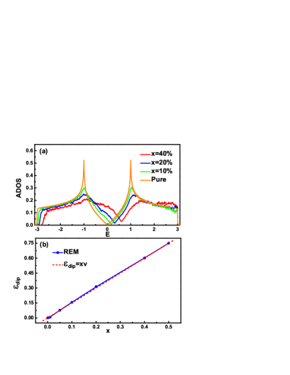
Figure 4: (Color online) (a) ADOS ($\rho$) of a graphene with various (number of disorders)impurity concentrations ($x$). Here, on-site potential is set to be $1.5$ ($v=1.5$). (b) The energy shift ($\varepsilon_{dip}$) as a function of impurity concentrations ($x$) (the blue solid line), for on-site potential $v=1.5$. The red dashed line shows the linear relation: $\varepsilon_{dip}=xv$.

Fig. 4(a) presents the calculated ADOS of a graphene with different impurity concentrations($x$) while the on-site potential ($v$) is set to be $1.5$. When the on-site potential ($v$) is small, the anti-resonance dip exists, but there is no obvious resonance peak. Interestingly, we find that the linear relation, $\varepsilon_{dip}$=$xv$, still holds even for a large impurity concentration, though the multiply scattering among impurities is strong. Generally, this linear relation can be easily understood by using virtual crystal approximation(VCA) which simply predicts a energy level at which two bands coincide is shifted by $\varepsilon_{dip}$=$xv$. The prediction of VCA is reasonable for a low impurity concentration and a small on-site potential, but it fails for large values. It is also found that the van Hove singularity disappears when the impurity concentration is about $40\%$. This reflects that the phenomenon of the spectrum rearrangement happens in the large impurity concentration.

In order to get better understanding of the linear relation, $\varepsilon_{dip}$=$xv$, here, we present a qualitative discussion based on the coherent potential approximation (CPA).The Self-energy $\Sigma$ can be obtained by neglecting multiple scattering process among the impurities as

$$\Sigma=\cfrac{xv}{1-vG_{0}(E-\Sigma)}$$ (14)

The energy shift $\varepsilon_{dip}$ can be determined by substituting $E-\Sigma$ =$i\kappa$ ($\kappa>0$ is real). Thus we have,

$$\varepsilon_{dip}\equiv Re\Sigma=\cfrac{xv(1-\cfrac{\sqrt{3}\kappa v}{3})}{(1-\cfrac{\sqrt{3}\kappa v}{3})^{2}+\cfrac{1}{3\pi_{2}}\kappa^{2}v^{2}\ln^{2}|\cfrac{\kappa^{2}}{9a^{2}k_{c}^{2}/4-\kappa^{2}}|}.$$ (15)

$\kappa$ is calculated by the following equation,

$$Im\Sigma=-\kappa=\cfrac{\cfrac{\sqrt{3}}{3\pi}\kappa v^{2}\ln|\cfrac{\kappa^{2}}{9a^{2}k_{c}^{2}/4-\kappa^{2}}|}{(1-\cfrac{\sqrt{3}\kappa v}{3})^{2}+\cfrac{1}{3\pi_{2}}\kappa^{2}v^{2}\ln^{2}|\cfrac{\kappa^{2}}{9a^{2}k_{c}^{2}/4-\kappa^{2}}|}.$$ (16)

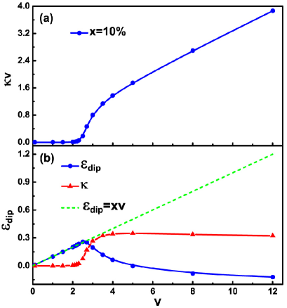
Figure 5: (Color online) (a) Parameter $\kappa v$ as a function of on-site potential ($v$), where impurity concentrations is $x=10\%$. (b) The energy shift ($\varepsilon_{dip}$) as the function of on-site potential ($v$). The blue and red solid lines stand for the results calculated using the recursion method and CPA, respectively. In the calculations, we choose $x=10\%$. The green dashed line indicates the linear relation, $\varepsilon_{dip}=xv$.

If $\kappa v\ll 1$, Eq. (15) can be simplified to $\varepsilon_{dip}$=$xv$. For a system with a given impurity concentration e.g.$10\%$, Fig. 6(a) clearly shows that $\kappa v$ is a small value for $v$ less than 2.5. If $\kappa v\ll 1$, the relation, $\varepsilon_{dip}$=$xv$, is correct as shown in Fig. 3(b). However, the calculated curve of $\varepsilon_{dip}$ using CPA does not match the linear relation ($\varepsilon_{dip}$=$xv$) when $v$ is larger than 2.5. The possible reason is that multiple scattering among the impurity cannot be neglected in the CPA calculations when $v>2.5$. With given the impurity concentration $10\%$, based on the condition of $|Re\Sigma|=|Im\Sigma|$, CPA calculation estimates roughly the threshold value $v_{dip}\approx 2.9$ of on-site potential ($v_{dip}$) to guarantee the linear relation. This result is somewhat underestimated by looking at Fig. 3(a), for instance, the value of $v_{dip}$ should be larger than 3. For the system with a given on-site potential ($v$), Fig. 6(a) shows that the results obtained using the CPA method are different from those obtained using the recursion method. In the case of $v=1.5$, the inequality $\kappa v\ll 1$ is satisfied only for $x\leq 0.2$. With small on-site potential, we find that the relation $\varepsilon_{dip}$=$xv$ still holds even when impurity concentration is close to $50\%$. This observation indicates that the CPA is not applicable to obtain the reliable results of graphene when impurity number is large because which neglects the scattering among impurities.

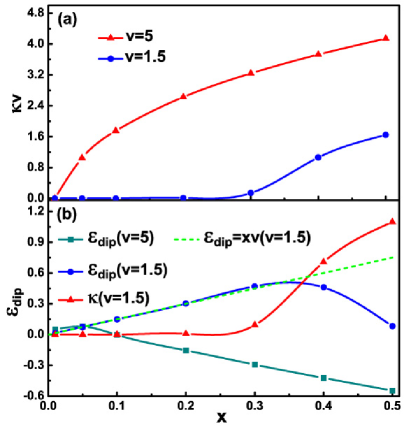
Figure 6: (Color online)(a) Parameter $\kappa v$ as a function of impurity concentration ($x$) when $v=1.5$ or $v=5$. (b) The energy shift ($\varepsilon_{dip}$) as a function of impurity concentration ($x$). The blue and dark cyan solid lines stand for the case when $v=1.5$ and $v=5$, respectively. The red solid line indicates $\kappa$ as a function of impurity concentration ($x$) for $v=1.5$ case. The green dashed line shows the linear relation of $\varepsilon_{dip}=xv$.

The threshold impurity concentration ($x_{dip}$) for $v=1.5$ is about $37\%$ when the liner relationship is correct, as show in Fig. 6(b). When the on-site potential ($v$) becomes large enough, $x_{dip}$ is extremely small. This result is consistent with our calculated results shown in Fig. 5. There is a visible dip only for extreme small impurity concentrations. Clearly, $x_{dip}$ is sensitive to the on-site potentials. When the inequality $\kappa v\ll 1$ does not hold anymore, $x_{dip}$ cannot be obtained through the simple CPA calculations.PRB07-Skr Previous theoretical studies PRB07-Skr ; PRB04-Skr have predicted that the CPA with single-site scattering may fail to predict the dip. Our results obtained by the recursion method prove that the CPA is valid only if ($\kappa v\ll 1$). The linear relation, $\varepsilon_{dip}$=$xv$, can be further extended to system with high impurity concentration and small on-site potential though the CPA fails to work.

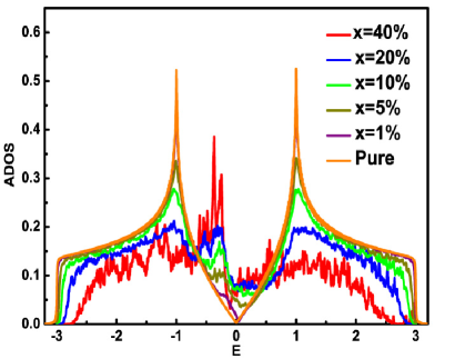
Figure 7: (Color online) The calculated ADOS ($\rho$) with various impurity concentration ($x$) in a graphene. Here, $v=5$.

For large on-site potentials as shown in Fig. 7, there are obvious resonance peaks. The height of the peak increases significantly as the number of disorders increases. However, the position of resonance peak does not shift obviously at high impurity concentration. These results suggest that $E_{r}$ is determined by the on-site potential ($v$) and impurity concentration ($x$). However, when the on-site potential is large, $E_{r}$ does not depend obviously on the impurity concentration even $x$ has large value. It is also found that the van Hove singularity disappears when the impurity concentration is about $20\%$.

The disordered graphene with a finite density of vacancies can be modeled by setting the on-site potential $v$ to a very large value.PRB07-Weh ; PRB06-Wang Fig. 8 shows the calculated ADOS of graphene systems with vacancies ($v=1000$) based on the recursion method. There is a clear sharp peak near the Dirac point, which is in line with the numerical results obtained using the stochastic recusive method.PRL06-Pere This sharp peak can be fit very well by the Lorentz distribution. However, the precious theoretical calculation, based on the full Born approximation (FBA),PRB06-Per predicted the value of ADOS should be exactly zero. Its error may occur because the multiple scattering is ignored in the FBA calculation. Meanwhile the calculation based on the CPACond-mat05-Per and the full self-consistent Born approximation (FSBA)PRB06-Per also fails to produce observable resonance peaks. These results indicate that there are some limitations in the CPA, FBA and FSBA methods near the Dirac point. The correctness or accuracy of these methods need to be further examined.

Figure 8: (Color online) The calculated ADOS ($\rho$) of graphene with different concentrations of vacancies. Here, we chose $v=1000$.

IV Conclusion

In this paper, these ADOS of a binary alloy disorder in disordered graphene are calculated using the recursion method. The applicability and accuracy of the recursion method are addressed. It is found that the shape of the resonance peak and the position of the anti-resonance dip are sensitive to impurity concentration ($x$) and on-site potential ($v$). The linear relation, $\varepsilon_{dip}$=$xv$, can be derived based on the CPA when $\kappa v\ll 1$. This relation is able to explain the position shift of anti-resonance dips at low or high impurity concentration for small on-site potential case. For large $v$, either the CPA or Eq. (14) fails except for extremely low impurity concentration ($\kappa v\ll 1$). The main reason for the failure of the CPA is that the scattering among impurities is neglected. By setting $v$ to be a huge value, the model can be used to simulates finite concentration of vacancies in a graphene. The resonance peak of ADOS at the dirac point is found.

References

- (1) K. S. Novoselov, A. K. Geim, S. V. Morozov, D. Jiang, Y. Zhang, S. V. Dubonos, I. V. Grigorieva, and A. A. Firsov, Science 306, 666 (2004).
- (2) K. S. Novoselov, A. K. Geim, S. V. Morozov, D. Jiang, M. I. Katsnelson, I. V. Grigorieva, S. V. Dubonos, A. A. Firsov, Nature(London) 438, 197 (2005).
- (3) Yuanbo Zhang, Yanwen Tan, Horst L. Stormer and Philip Kim, Nature(London) 438, 201 (2005).
- (4) N. M. R. Peres, F. Guinea, A. H. Castro Neto, cond-mat/0506709.
- (5) N. M .R. Peres, F. Guinea, and A. H. Castro Neto, Phys. Rev. B 73, 125411 (2006).
- (6) M. I. Katsnelson, Eur. Phys. J. B 51, 157 (2006).
- (7) J. Cserti, Phys. Rev. B 75, 033405 (2007).
- (8) K. Ziegler , Phys. Rev. Lett. 97, 266802 (2007).
- (9) V.P. Gusynin and S.G. Sharapov, Phys. Rev. B 73, 245411 (2006).
- (10) K. Ziegler, Phys. Rev. B 75, 233407 (2007).
- (11) Kentaro Nomura and A. H. MacDonald, Phys. Rev. Lett. 98, 076602 (2007).
- (12) K. h. Han, D. Spemann, P. Esquinazi, R. Höhne, R. Riede, and T. Butz, Adv. Mater. (Weinheim, Ger.) 15 (20), 1719 (2003).
- (13) M. A. H. Vozmediano, M. P. L pez-Sancho, T. Stauber and F. Guinea, Phys. Rev. B 72, 155121 (2005).
- (14) R. Tamura and M. Tsukada, Phys. Rev. B 55, 4991 (1997).
- (15) T. Nakanishi and T. Ando, J. Phys. Soc. Jpn. 66, 2973 (1997).
- (16) Y. Kopelevich, P.Esquinazi, J.H.S Torres, and S. Moehlecke, J. Low Temp. Physics 119, 691 (2000).
- (17) A. A. Ovchinnikov and I. L. Shamovsky, J. Mol. Struct., Theochem 251, 133 (1991).
- (18) Jos Gonz lez, Francisco Guinea, and M. Angeles H. Vozmediano, Phys. Rev. Lett. 69, 172 (1992).
- (19) J. C. Charlier, T. W. Ebbesen and Ph. Lambin, Phys. Rev. B 53, 11108 (1996).
- (20) K. Wakabayshi and M. Sigrist, Phys. Rev. Lett. 84, 3390 (2000).
- (21) K. Wakabayshi, Phys. Rev. B 64, 125428(2001).
- (22) J. Gonz lez, F. Guinea and M. A. H. Vozmediano, Phys. Rev. B 63, 134421(2001).
- (23) K. Harigaya , J. Phys. Condens. Matter 13, 1295 (2001).
- (24) H. Matsumura and T. Ando, J. Phys. Soc. Jpn. 70, 2657 (2001).
- (25) K. Harigaya, A. Yamashiro, Y. Shimoi, K. Wakabayashi, Y. Kobayashi, N. Kawatsu, K. Takai, H. Sato, J. Ravier, T. Enoki, M. Endo, J. Phys. Chem. Solids 65, 123 (2004).
- (26) Elizabeth J. Duplock,Matthias Scheffler,and Philip J. D. Lindan, Phys. Rev. Lett. 92, 225502 (2004).
- (27) P. O. Lehtinen, A. S. Foster, Yuchen Ma, A. V. Krasheninnikov, and R. M. Nieminen, Phys. Rev. Lett. 93, 187202 (2004).
- (28) W. M. Hu, J. D. Dow, and C. W. Myles, Phys. Rev. B 30, 1720 (1984).
- (29) Yu. V. Skrypnyk and V. M. Loktev, Phys. Rev. B 73, 241402(R) (2006).
- (30) Yu. V. Skrypnyk and V. M. Loktev, Phys. Rev. B 75, 245401 (2007).
- (31) Yu. G. Pogorelov, cond-mat/0603327v1.
- (32) T. O. Wehling, A. V. Balatsky, M. I. Katsnelson, A. I. Lichtenstein, K. Scharnberg,and R. Wiesendanger, Phys. Rev. B 75, 125425 (2007).
- (33) Vitor M. Pereira, F. Guinea, J. M. B. Lopes dos Santos, N. M. R. Peres, and A. H. Castro Neto, Phys. Rev. Lett. 96, 036801 (2006).
- (34) Yu. V. Skrypnyk, Phys. Rev. B 70, 212201 (2004).
- (35) I. M. Lifshiz, Adv. Phys. 13, 483 (1964).
- (36) Lanczos, C., 1950, J. Res. Nat. Bur. Stand. 45, 255 (1950).
- (37) Haydock R., Heine V. and Kelly M. J., J. Phys. C: Solid St. Phys. 5, 2845 (1972).
- (38) Haydock R., Heine V. and Kelly M. J., J. Phys. C: Solid St. Phys. 8, 2591 (1975).
- (39) J. J. Sinai, C. Wongtawatnugool and S. Y. Wu, Phys. Rev. B 26, 1829 (1982).
- (40) R. Haydock and R. L. Te, Phys. Rev. B 49, 10845 (1994).
- (41) D. J. Lohrmann, L. Resca, G. P. Parravicini and R. D. Graft,Phys. Rev. B 40, 8404 (1989).
- (42) Z. F. Wang, Ruoxi Xiang, Q. W. Shi, Jinlong Yang, Xiaoping Wang, J. G. Hou, and Jie Chen, Phys. Rev. B 74, 125417 (2006).