Super- and subradiant emission of two-level systems in the near-Dicke limit

Abstract

We analyze the stability of super- and subradiant states in a system of identical two-level atoms in the near-Dicke limit, i.e., when the atoms are very close to each other compared to the wavelength of resonant light. The dynamics of the system are studied using a renormalized master equation, both with multipolar and minimal-coupling interaction schemes. We show that both models lead to the same result and, in contrast to non-renormalized models, predict that the relative orientation of the (co-aligned) dipoles is unimportant in the Dicke limit. Our master equation is of relevance to any system of dipole-coupled two-level atoms, and gives bounds on the strength of the dipole-dipole interaction for closely spaced atoms. Exact calculations for small atom systems in the near-Dicke limit show the increased emission times resulting from the evolution generated by the strong dipole-dipole interaction. However, for large numbers of atoms in the near-Dicke limit, it is shown that as the number of atoms increases, the effect of the dipole-dipole interaction on collective emission is reduced.

I Introduction

Collective spontaneous emission from dense atomic systems has been of interest since the pioneering work of Dicke Dicke (1954) who predicted that co-located two-level systems (or qubits) possess collective quantum states in which spontaneous emission is enhanced (superradiance) or suppressed (subradiance). Subradiant states, which form an example of spontaneous emission cancellation Marzlin et al. (2007), are of interest for quantum information processing because they form an example of decoherence-free subspaces (DFS) and subsystems Kempe et al. (2001); Lidar et al. (1998); Zanardi and Rasetti (1997). DFSs can be used to encode against system-environment interactions that can cause loss of quantum information. In the Dicke model, the system is formed by a collection of two-level systems coupled to the vacuum radiation field. To achieve infinite lifetime quantum information storage, the Dicke limit of co-located two-level atoms is necessary Karasik et al. (2007), but for practical implementations of quantum processors a small separation is unavoidable and the corresponding decoherence needs to be taken into account Brooke (2007). Also, the result derived in Ref. Karasik et al. (2007) implies that exact superradiant behaviour does not exist outside of co-located atomic systems—it is not possible to observe perfect superradiance. So, our results have dual applicability to both tests of superradiance and coherent control of atomic systems for quantum information.

An important question for the design of a quantum processor that makes use of subradiant states is the trade-off between spontaneous emission suppression on one hand and the increase of the dipole-dipole interaction between different two-level systems on the other hand. This question is difficult to answer because (i) at very short distances the details of the interaction will strongly depend on the actual physical particles that are modelled by the two-level system, and (ii) the energy level shifts due to the coupling between different two-level systems formally diverges in the Dicke limit. Point (i) can only be addressed by performing an ab initio calculation for a specific system—an effort that is only justified when a promising candidate for DFS-based quantum information processing is found. Part of the purpose of this paper is to resolve point (ii) by providing a renormalized theory of the interaction of closely spaced two-level systems.

The master equation we derive here is applicable to any system of dipole-coupled qubits. There have been a number of examples of quantum processors that exploit a dipole-dipole interaction, e.g., Beige et al. (2000); Brennen et al. (2000); Petrosyan and Kurizki (2002); Brooke (2007); Kiffner et al. (2007), all of which rely on the formally divergent result derived in Refs. Belavkin et al. (1969); Lehmberg (1970a, b); Agarwal (1970) and therefore can only be applied for sufficiently large separation between the atoms. Our result allows the analysis of quantum processors to be extended to the near-Dicke limit.

In this paper, we use the regularized master equation to study the effect of the dipole-dipole interaction in the near-Dicke limit. Previous work has approximated the dynamics of closely separated atoms using the (divergent) contact interaction, and shown that dipole-dipole interactions dramatically upset the predictions of the Dicke model Gross and Haroche (1982); Carmichael and Kim (2000). Here, we present a renormalized model that is applicable in the near-Dicke limit, and we apply the result to various atomic systems. For three atoms, we explicitly show the population transfer, caused by the dipole-dipole interaction, between states in the one-quantum subspace in the near-Dicke limit. For five atoms, we use quantum trajectories, and show that in the near-Dicke limit, the waiting time distribution of the final photon is extended because the dipole-dipole interaction causes population transfer between the super- and subradiant Dicke states. The angular distribution confirms this, with less photons emitted along the interatomic axis when the dipole-dipole interaction is included in the evolution. For $N$ atoms, we make sensible approximations and find that—for a linear configuration—as the number of atoms increases the collective spontaneous emission timescale begins to dominate the population mixing timescale that is given by the strength of the dipole-dipole interaction.

The paper is organised as follows. In Sec. II we describe the model and present the regularized master equation for $N$ two-level atoms coupled to the radiation field. In Sec. III, we propose a value for both the transverse and longitudinal regularization parameter, both of which are based on physical considerations. In Sec. IV we show several results. First, that super- and subradiant emission properties are unaffected by the dipole-dipole interaction in the exact Dicke limit. Second, we demonstrate the mixing properties for closely-spaced small atom systems. Third, we show that for five atoms the emission direction is not significantly affected by the presence of a strong dipole-dipole interaction in the near-Dicke limit. Finally, we show that, in the near-Dicke limit, as the number of atoms increases, the detrimental effect of the dipole-dipole interaction on superradiance is reduced. In Appendix A, we derive a regularized expression for the dynamics of a system of $N$ 2LAs coupled to a quantized electric field at zero temperature in the minimal-coupling picture. Due to the popularity of the master equation in the electric-dipole picture, in App. B we derive the same result using the electric-dipole picture, showing that it does not matter which description of the electric-field one uses. The major difference between the methods is the order of the divergence that needs to be regularized, and the treatment of the static dipole-dipole interaction.

II Regularized master equation for $N$ two-level atoms

We consider a system of $N$ two-level atoms interacting with the free radiation field, which initially occupies the vacuum state. The interaction with the field induces a dipole-moment in the atoms, and these induced dipoles are allowed to interact via photon exchange. For each atom, the matrix elements of the dipole operator are given by the same vector ${\bm{d}}\equiv\langle e|\hat{{\bm{d}}}|g\rangle$. In absence of the interaction, the atomic system’s Hamiltonian is given by

$$\widehat{H}_{\text{s}}=\frac{\hbar\omega_{0}}{2}\sum_{n=1}^{N}\hat{\sigma}_{nz}\;,$$ (1)

with $\omega_{0}\equiv({\cal E}_{e}-{\cal E}_{g})/\hbar$ the resonance frequency, ${\cal E}_{i}$ the atomic energy levels, and $\hat{\sigma}_{nz}$ the Pauli z-matrix for the $n^{\text{th}}$ atom. We assume that the latter is located at position ${\bm{r}}_{n}$ and use $\bm{r}_{nm}\equiv\bm{r}_{n}-\bm{r}_{m}$ to denote the distance vector between a pair $(n,m)$ of atoms.

For such a system of two-level atoms it is possible to derive a Markovian master equation in which the influence of the radiation field is described by a set of atomic decay rates, energy shifts, and coupling terms. Belavkin et al. (1969); Lehmberg (1970a); Agarwal (1970); Carmichael and Kim (2000); Clemens et al. (2003). However, for closely spaced atoms it is necessary to regularize and renormalize these parameters. Using minimal coupling (see App. A) and electric dipole coupling (see App. B) we have derived a regularized master equation to describe the dynamics of the density matrix $\rho$ of an ensemble of atoms in the near-Dicke limit. The results of both calculations agree (see Sec. B) and yield

$$\dot{\rho}= -\frac{\text{i}}{\hbar}[\widehat{H}_{\text{s}},\rho]-\text{i}\sum_{n,m=1}^{N}(\tilde{\Delta}^{\perp}_{nm}+\tilde{\Delta}^{\parallel}_{nm})[\hat{\sigma}_{n+}\hat{\sigma}_{m-},\rho]$$

$$+\sum_{n,m=1}^{N}\tilde{\gamma}_{nm}(2\hat{\sigma}_{m-}\rho\hat{\sigma}_{n+}-\hat{\sigma}_{n+}\hat{\sigma}_{m-}\rho-\rho\hat{\sigma}_{n+}\hat{\sigma}_{m-})\;.$$ (2)

This equation has the same structure as the non-regularized master equation, but the energy shifts $\tilde{\Delta}^{\perp}_{nm}$ and $\tilde{\Delta}^{\parallel}_{nm}$, which describe the dynamic (or transverse) and static (or longitudinal) contribution to the dipole-dipole interaction, remain finite as the distance between the atoms goes to zero. For $n=m$ they correspond to the Lamb shift for two-level systems (see App. A). The quantity $\tilde{\gamma}_{nm}$ describes a collective spontaneous emission effect, i.e., incoherent de-excitation of the collective atomic state.

To facilitate the physical interpretation of Eq. (II), we first state the non-regularized expressions for these parameters,

$$\gamma_{nm} =\frac{3}{4}\gamma\{\alpha(\xi_{nm})+\eta_{nm}\beta(\xi_{nm})\},$$ (3)

$$\Delta_{nm}^{\perp}= \frac{3}{4}\gamma\Bigg{\{}(\eta_{nm}-1)\frac{\cos\xi_{nm}}{\xi_{nm}}+(1-3\eta_{nm})$$

$$\times\left(\frac{\sin\xi_{nm}}{\xi_{nm}^{2}}+\frac{\cos\xi_{nm}}{\xi_{nm}^{3}}\right)\Bigg{\}}-\Delta^{\parallel}_{nm},$$ (4)

$$\Delta^{\parallel}_{nm} =\frac{3\gamma(1-3\eta_{nm})}{4\xi_{nm}^{3}},$$ (5)

which we denote by the same symbols as the regularized parameters but without tilde. In the limit of small $\xi_{nm}\equiv k_{0}\,r_{nm}$, the parameter $\gamma_{nm}$ approaches $\gamma/2$, where $\gamma=k_{0}^{3}|\bm{d}|^{2}/(3\pi\varepsilon_{0}\hbar)$ denotes the spontaneous emission rate of an isolated atom in free space, with $k_{0}=\omega_{0}/c$ the wavenumber of resonant light. The two functions

$$\alpha(x) \equiv\frac{\cos x}{x^{2}}-\frac{\sin x}{x^{3}}+\frac{\sin x}{x},$$ (6)

$$\beta(x) \equiv 3\frac{\sin x}{x^{3}}-3\frac{\cos x}{x^{2}}-\frac{\sin x}{x},$$ (7)

describe the emission pattern of a radiating dipole. The directional dependence of the dipole-dipole interaction is expressed through the parameter $\eta_{nm}\equiv(\bm{d}\cdot\bm{r}_{nm})^{2}/(|\bm{d}|^{2}r_{nm}^{2})$. The longitudinal energy shift $\Delta^{\parallel}_{nm}$ corresponds to the Coulomb interaction energy between two static point dipoles. It is exactly cancelled by a corresponding term in the transverse energy shift $\Delta_{nm}^{\perp}$ so that their sum (the curly parentheses in Eq. (4) ) is retarded.

The result for the corresponding regularized quantities is somewhat more involved,

$$\tilde{\gamma}_{nm} =\frac{3}{4}\tilde{\gamma}[\alpha(\xi_{nm})+\eta_{nm}\beta(\xi_{nm})],$$ (8)

$$\tilde{\Delta}^{\perp}_{nm} =\frac{3}{4}\tilde{\gamma}\Bigg{\{}\frac{\text{e}^{-r_{nm}\Lambda_{\perp}}}{k_{0}r_{nm}^{3}}\bigg{(}\frac{(1-3\eta_{nm})(1+r_{nm}\Lambda_{\perp})}{\Lambda_{\perp}^{2}}$$

$$+(1-\eta_{nm})r_{nm}^{2}\bigg{)}+(\eta_{nm}-1)\frac{\cos\xi_{nm}}{\xi_{nm}}+(1-3\eta_{nm})$$

$$\times\left(\frac{\sin\xi_{nm}}{\xi_{nm}^{2}}+\frac{\cos\xi_{nm}}{\xi_{nm}^{3}}-\frac{k_{0}^{2}+\Lambda_{\perp}^{2}}{\Lambda_{\perp}^{2}\xi_{nm}^{3}}\right)\Bigg{\}},$$ (9)

$$\tilde{\Delta}^{\parallel}_{nm} =\frac{3\gamma\text{e}^{-\frac{r_{nm}\Lambda_{\parallel}}{\sqrt{2}}}}{8\xi^{3}_{nm}}\Bigg{\{}\text{e}^{\frac{r_{nm}\Lambda_{\parallel}}{\sqrt{2}}}(2-6\eta_{nm})+(3\eta_{nm}-1)$$

$$\times(2+\sqrt{2}r_{nm}\Lambda_{\parallel})\cos\frac{r_{nm}\Lambda_{\parallel}}{\sqrt{2}}+r_{nm}\Lambda_{\parallel}(3\sqrt{2}\eta_{nm}$$

$$-\sqrt{2}+2r_{nm}\eta_{nm}\Lambda_{\parallel})\sin\frac{r_{nm}\Lambda_{\parallel}}{\sqrt{2}}\Bigg{\}},$$ (10)

where

$$\tilde{\gamma} =\gamma\frac{\Lambda_{\perp}^{2}}{\Lambda_{\perp}^{2}+k_{0}^{2}},$$ (11)

but we will see below that in the near-Dicke limit it admits a simple physical interpretation after renormalization. The regularization parameters $\Lambda_{\parallel}$ and $\Lambda_{\perp}$, which will be fixed by a renormalization procedure (Sec. III), describe the cut-off scales in the regularized theory: photons with wave-numbers larger than $\Lambda_{\parallel},\Lambda_{\perp}$ no longer contribute to the interaction.

The regularization performed here leads to a self-consistent model that is suitable for a qualitative description of the emission dynamics of $N$ 2LAs in the near-Dicke limit. Its range of validity extends to atomic separations that are much smaller than the wavelength of resonant light, but large enough so that the electronic clouds of the atoms do not overlap and the atoms interact like point dipoles.

We remark that our analysis of the master equation extends only to second order in the interaction Hamiltonian and therefore does not include higher-order effects such as a van der Waals interaction. It is impossible to give a general estimate of when these effects can no longer be neglected. One reason is that such interactions can be important for one physical process, but unimportant for another. For instance, the van der Waals interaction may be of relevance for the interaction between ground-state atoms, a state in which the atoms do not possess a dipole moment, but may be negligible for the interaction between atoms that are polarized by a light field. Another reason is that the significance of interactions other than dipole-dipole depends heavily on the atomic species, or even atomic states, under consideration. For example, the van der Waals interaction can induce significant energy shifts at separations as large as a few micrometers if the atoms are prepared in a Rydberg state Singer et al. (2005). So, for a full analysis of closely separated atoms that would accurately predict experimental results for a given atomic species, an electronic many-body problem that takes all energy levels (including the continuum) into account would need to be solved. Such a calculation is a formidable task and beyond the aim of this paper, which is to provide a qualitative model for dipole-interacting two-level systems.

III Renormalization

The transverse and longitudinal parts of the master equation represent the propagating and nonpropagating parts of the dipole-dipole interaction. So, the two regularization parameters, $\Lambda_{\perp}$ and $\Lambda_{\parallel}$, have different values.

III.1 Transverse

In Sec. A we have shown that the divergence of $\Delta^{\perp}_{nm}$ for small atomic separations and the divergence of the two-level Lamb shift $\Delta_{\text{Lamb}}^{\text{(2-lev)}}$ share the same origin. In both cases, a virtual photon is emitted by one atom and later re-absorbed; in the case of $\Delta_{\text{Lamb}}^{\text{(2-lev)}}$ it is re-absorbed by the same atom, in the case of the dynamic dipole-dipole interaction $\Delta^{\perp}_{nm}$ it is re-absorbed by a different atom. For this reason, we regularize both quantities using the same parameter $\Lambda_{\perp}$, and fix its value by renormalizing the Lamb shift of a single two-level atom. We begin by recalling Bethe’s famous argument for the calculation of the Lamb shift Bethe (1947).

Using second-order perturbation theory, the shift in the atomic level $\mathinner{|{a}\rangle}$ due to the interaction Hamiltonian (45), for $N=1$ particle, is given by

$$\Delta\mathcal{E}_{a}=\frac{1}{6\pi^{2}\varepsilon_{0}\hbar c^{3}}\sum_{b\neq a}|\bm{d}_{ba}|^{2}\omega_{ab}^{2}\int_{0}^{\infty}\frac{\text{d}\mathcal{E}\mathcal{E}}{\hbar\omega_{ab}-\mathcal{E}}.$$ (12)

where $\omega_{ab}=(\mathcal{E}_{a}-\mathcal{E}_{b})/\hbar$ and we have made use of Eq. (40). This expression is infinite and requires renormalization. The energy of the free-electron due to its coupling to the field is

$$\Delta\mathcal{E}^{\text{free}}_{a}=-\frac{1}{6\pi^{2}\varepsilon_{0}\hbar c^{3}}\sum_{b\neq a}|\bm{d}_{ba}|^{2}\omega_{ab}^{2}\int_{0}^{\infty}\text{d}\mathcal{E}.$$ (13)

Bethe proposed that the observed energy shift for $\mathinner{|{a}\rangle}$ should be the difference between the energy of the free-electron and the bound electron

$$\Delta\mathcal{E}_{a}^{\text{obs}} =\Delta\mathcal{E}_{a}-\Delta\mathcal{E}^{\text{free}}_{a},$$

$$=\frac{1}{6\pi^{2}\varepsilon_{0}c^{3}}\sum_{b\neq a}|\bm{d}_{ba}|^{2}\omega_{ab}^{3}\int_{0}^{\infty}\frac{\text{d}\mathcal{E}}{\hbar\omega_{ab}-\mathcal{E}}.$$ (14)

The divergence in Eq. (12) has been reduced from linear to logarithmic. Bethe proposed a cut-off to the integration that embodies the assumption that the main part of the Lamb shift is due to the interaction of the electron with vacuum modes of frequency small enough to justify a nonrelativistic approach. Naturally, he took this cut-off to be $mc^{2}$

$$\Delta\mathcal{E}_{a}^{\text{obs}} \simeq\frac{1}{6\pi^{2}\varepsilon_{0}c^{3}}\sum_{b\neq a}|\bm{d}_{ba}|^{2}\omega_{ba}^{3}\ln\frac{mc^{2}}{\hbar|\omega_{ba}|},$$ (15)

for $mc^{2}>|\mathcal{E}_{b}-\mathcal{E}_{a}|$.

At this point, our derivation differs from that performed by Bethe. Because our model is based on two-level systems only, the sum in Eq. (15) contains only a single term ($b=1$ for $a=0$ and vice versa). So, in our model the Lamb-shift for a 2LA is given by

$$\Delta\mathcal{E}_{\text{2LA}} =\Delta\mathcal{E}_{1}-\Delta\mathcal{E}_{0},$$

$$=\frac{\hbar\gamma}{\pi}\ln\frac{\lambda}{\lambda_{c}},$$ (16)

for $\lambda_{c}=2\pi\hbar/mc$ the Compton wavelength and $\lambda$ the wavelength of resonant light. Equating with $\Delta_{\text{Lamb}}^{\text{(2-lev)}}$ of Eq. (56) gives

$$\Lambda_{\perp}\simeq\frac{2\pi}{\lambda_{c}},$$ (17)

where $\tilde{\gamma}\simeq\gamma$. Thus, $\Lambda_{\perp}/k_{0}\approx 10^{5}$ and $\Lambda_{\perp}$ cuts off the higher frequency vacuum modes.

III.2 Longitudinal

Within the dipole approximation, resonant light cannot resolve the microscopic structure of the 2LAs. The $r_{nm}^{-3}$ behaviour of the dipole-dipole interaction (4) can then be considered to apply only for $r_{nm}>a$, where $a$ is some microscopic length. The cut-off parameter has units of inverse length; we therefore estimate $\Lambda^{\parallel}$ to be

$$\Lambda^{\parallel}=\sqrt[3]{\frac{1}{V_{0}}},$$ (18)

where $V_{0}=\tfrac{4}{3}\pi a_{0}^{3}$ for $a_{0}$ the Bohr radius. This choice is in agreement with the estimate of Ref. de Vries et al. (1998) which is based on a $T$-matrix approach for scattering of classical light from point particles. At separations smaller than $a_{0}$, the dipole approximation breaks down, and the Lehmberg-Agarwal master equation is no longer an appropriate description of the physical system.

III.3 Comparison between regularized and non-regularized interaction

For interatomic distances that are not substantially smaller than the resonant wavelength $\lambda$ the predictions of the renormalized and non-renormalized master equations agree (see Fig. 1). This agreement results because renormalization only affects the description of a system at short scales. However, in the near-Dicke limit there are substantial differences between the two models.

The expansion of the decay rate and energy shifts to first order in the interatomic distance $\xi_{nm}=k_{0}\,r_{nm}$ is given by

$$\tilde{\Delta}^{\parallel}_{nm} = \frac{\gamma}{4\sqrt{2}}\frac{\Lambda_{\parallel}^{3}}{k_{0}^{3}}-\frac{3\gamma(1+\eta_{nm})}{32}\frac{\Lambda_{\parallel}^{4}}{k_{0}^{4}}\xi_{nm},$$ (19)

$$\tilde{\Delta}^{\perp}_{nm} = -\frac{\gamma}{2k_{0}}\frac{\Lambda_{\perp}^{3}}{k_{0}^{2}+\Lambda_{\perp}^{2}}+\frac{3\gamma(3-\eta_{nm})}{32}\frac{\Lambda_{\perp}^{2}}{k_{0}^{2}}\xi_{nm},$$ (20)

$$\tilde{\gamma}_{nm} = \frac{\gamma}{2}\frac{\Lambda_{\perp}^{2}}{k_{0}^{2}+\Lambda_{\perp}^{2}}\;.$$ (21)

Hence, the decoherence part of the master equation, which is proportional to $\tilde{\gamma}_{nm}$, takes the same form as in the exact Dicke limit. For $\Lambda_{\perp}\gg k_{0}$, deviations of $\tilde{\gamma}_{nm}$ from the single-atom emission rate $\gamma/2$ are only significant for larger distances $\xi_{nm}\gtrsim 1$.

The differences between the energy shift of the renormalized and the non-renormalized master equation are substantial, however. In contrast to the non-renormalized case, the dipole-dipole interaction does not diverge in the renormalized model. The reason for this is that the process of regularizing a theory can be considered as ignoring the detailed structure of a charge distribution on scales smaller than $1/\Lambda$. Equivalently, we can think of the charge distribution being smeared out on this scale. While the interaction energy can diverge for point charges as they approach each other, it remains finite for a proper (smooth, finite) charge distribution. Physically, atoms are composed out of many charged particles, and the details of this charge distribution are neither captured by the non-renormalized nor by the renormalized model. However, the renormalized model is a more appropriate model on scales larger than $1/\Lambda$ because it correctly describes measurable physical quantities such as the Lamb shift (see above) or the static atomic polarizability de Vries et al. (1998).

Furthermore, the non-renormalized theory not only predicts that the energy shift diverges, but that it diverges differently depending on the position of the atoms relative to the orientation of their dipole moment. Hence, it would make a difference whether the atoms approach the Dicke limit along the direction of the dipole moment or perpendicular to it. This is expressed through the parameter $\eta_{nm}$ and can be seen in Fig. 1. On the other hand, the renormalized master equation predicts that the value of the interaction energy for $\xi_{nm}\rightarrow 0$ is independent of the relative position of the atoms. This is a fundamentally different qualitative behaviour.

To shed light on why the dipole-dipole interaction in Dicke limit does not depend on the orientation of the (co-aligned ) dipoles, we again consider polarized atoms as smeared-out dipolar charge distributions. For illustrational purposes we think of atoms as homogeneously polarized spheres, but any other charge distribution would work as well as long as it is the same for all atoms. If the spheres are separated their interaction energy will depend on the orientation of the distance vector between both spheres relative to their dipole moment. However, when the spheres are perfectly overlapping, the distance vector is zero and the notion of its orientation becomes meaningless.

The preceeding argument explains why there should be no orientation dependence if we instantaneously place two co-aligned dipoles at the same position. However, the physical process of moving the dipoles to a common position may induce some memory in the system (a kind of “hysteresis”). In fact, the non-renormalized model cannot make any sensible statement about co-located dipoles because the energy shift is infinite, and it is only when we think of the two dipoles approaching each other from different directions that its prediction of an orientation dependence may appear reasonable. However, this idea is refuted if one considers two polarized spheres: regardless of how the spheres are brought together, in the Dicke limit their interaction energy should always be the same .

Figure 1: $\hbar\tilde{\Delta}^{\perp}_{nm}$ (dotted line), $10^{4}\hbar\tilde{\Delta}^{\parallel}_{nm}$ (solid line), and non-regularized $\Delta_{nm}^{\perp}+\Delta_{nm}^{\parallel}$ (dashed line) in units of the ground state energy ${\cal E}_{0}$ for (a) $\eta_{nm}=0$ and (b) $\eta_{nm}=1$.

For the particular values of the regularization parameters introduced above we have $\Lambda_{\perp},\Lambda_{\parallel}\gg k_{0}$. If we assume that the atomic dipole moment takes the value $|{\bm{d}}|=qa_{0}$, with $a_{0}=4\pi\hbar^{2}\varepsilon_{0}/(mq^{2})$ the Bohr radius, the expansion of decay rate and energy shifts take the form

$$\tilde{\Delta}^{\parallel}_{nm} = \frac{{\cal E}_{0}}{2\pi\hbar}\left(\frac{1}{\sqrt{2}}-\frac{1+\eta_{nm}}{8}\frac{3^{\frac{4}{3}}}{2^{\frac{2}{3}}\pi^{\frac{1}{3}}}\frac{r_{nm}}{a_{0}}\right),$$ (22)

$$\tilde{\Delta}^{\perp}_{nm} = \frac{\gamma}{2}\frac{\lambda}{\lambda_{c}}\left(-1+(3-\eta_{nm})\frac{3\pi}{8}\frac{r_{nm}}{\lambda_{c}}\right),$$ (23)

$$\tilde{\gamma}_{nm} = \frac{\tilde{\gamma}}{2}\;,$$ (24)

with ${\cal E}_{0}=mq^{4}/(8h^{2}\varepsilon_{0}^{2})$ the modulus of the hydrogen atom’s ground state energy. Thus, for our choice of renormalization parameters $\tilde{\Delta}^{\perp}_{nm}$ varies on the scale of the Compton wavelength but is much smaller than $\tilde{\Delta}^{\parallel}_{nm}$, which varies on the scale of the Bohr radius.

Figure 2: Double-logarithmic plot of the moduli of $\hbar\tilde{\Delta}^{\perp}_{nm}$ (dotted line), $\hbar\tilde{\Delta}^{\parallel}_{nm}$ (solid line), and non-regularized $\Delta_{nm}^{\perp}+\Delta_{nm}^{\parallel}$ (dashed line) in units of the ground state energy ${\cal E}_{0}$ for (a) $\eta_{nm}=0$ and (b) $\eta_{nm}=1$.

Fig. 1 (Fig. 2) shows the energy shifts (modulus of the energy shifts) as a function of the distance between two atoms. The sharp dips in Fig. 2 indicate a sign change in the energy shifts. As can be seen from Eqs. (4) and (5), the shifts oscillate with a period of $2\pi/k_{0}$, which corresponds to the wavelength of resonant light. That the dips do not approach zero is an artifact of the double-logarithmic plot. At distances $\xi_{nm}\lesssim 0.5\times 10^{-3}$, $\tilde{\Delta}_{nm}^{\perp}$ begins to differ significantly from $\Delta_{nm}^{\perp}+\Delta_{nm}^{\parallel}$. The region between this length scale and the scale $a_{0}$ at which the atoms start to overlap corresponds to the near-Dicke limit. This is the range in which our theory is applicable and provides qualitatively different predictions as compared to the non-renormalized master equation.

Another interesting aspect of the energy shifts can be seen in Fig. 2. For distances $\xi_{nm}>0.5\times 10^{-3}$, the sum $\tilde{\Delta}_{nm}^{\perp}+\tilde{\Delta}_{nm}^{\parallel}$ agrees with the non-renormalized dipole-dipole interaction $\Delta_{nm}^{\perp}+\Delta_{nm}^{\parallel}$. To achieve this agreement for all $\xi_{nm}>0.5\times 10^{-3}$, both the transverse (or dynamic) and the parallel (or static) energy shift need to be taken into account. However, in the region $\xi_{nm}<1$ the dipole-dipole interaction is almost completely generated by the static energy shift, while for $\xi_{nm}>1$ it is generated by the dynamic energy shift. This is reminiscent of the well-known fact that the near-field of an oscillating dipole corresponds to the static dipole field times an oscillating factor.

IV Emission dynamics

Earlier work using the divergent dipole-dipole interaction has provided a number of insights into super- and subradiance. In Ref. Coffey and Friedberg (1978) Coffey and Friedberg studied the case of two and three atoms and showed that the dipole-dipole interaction causes population transfer between the super- and subradiant Dicke states. The authors proposed a timescale, $\mathcal{O}(\xi^{-3})$, for which the effects of superradiance are dampened. In Ref. Gross and Haroche (1982) Gross and Haroche described how the dipole-dipole interaction generally breaks the permutation symmetry of the atom-field couplings due to differences in the close-neighbor environment of the different 2LAs. They also examined the explicit example of three 2LAs. Outside the near-Dicke limit, Clemens et al. Clemens et al. (2003) showed that the emission of the final photon from a line of atoms showed an angular dependence, and that this was not effected quantitatively by dipole-dipole interactions.

Using the results derived in the previous section, for the first time we can investigate the effect of the dipole-dipole interaction on the superradiance of atoms in the near-Dicke limit. We show that in the exact Dicke limit, in the presence of a dipole-dipole interaction, the emission is superradiant. Next, we show the effect of the dipole-dipole interaction on the population of the Dicke states in the near-Dicke limit for three and five 2LAs in a linear configuration. Then, we show that in the near-Dicke limit a strong dipole-dipole interaction does not quantitatively affect the emission direction, but the probability of emission is reduced. Next, we study $N$-atom systems and find that, contrary to expectations, the denser the atomic system (within the regime considered here), the greater the likelihood that superradiance will dominate the emission characteristics.

Before examining the emission dynamics in the near-Dicke limit, we show that in the Dicke limit, the dipole-dipole interaction does not affect the emission dynamics. The bare Hamiltonian, $\widehat{H}_{\text{b}}$, is

$$\widehat{H}_{\text{b}}=\hbar\omega_{0}\widehat{R}_{z}\qquad\text{with}\qquad\widehat{R}_{z}\equiv\sum_{n=1}^{N}\frac{\widehat{\sigma}_{nz}}{2},$$ (25)

for $N$ co-located atoms. The renormalized dipole-dipole interaction Hamiltonian of Eq. (II) takes the form

$$\widehat{H}_{\text{d}}=\sum^{N}_{n,m=1}(\tilde{\Delta}^{\perp}_{nm}+\tilde{\Delta}^{\parallel}_{nm})\widehat{\sigma}_{n\textrm{\tiny{+}}}\widehat{\sigma}_{m-}.$$ (26)

In the near Dicke limit we can expand this expression to first order in the interatomic distance. Eqs. (22, 23) yield

$$\tilde{\Delta}^{\perp}_{nm}+\tilde{\Delta}^{\parallel}_{nm} \approx\tilde{\Delta}_{0}+\tilde{\Delta}_{1,nm},$$ (27)

$$\tilde{\Delta}_{0} \approx\frac{{\cal E}_{0}}{2\sqrt{2}\pi\hbar},$$ (28)

$$\tilde{\Delta}_{1,nm} \approx\frac{{\cal E}_{0}}{2\pi\hbar}\frac{1+\eta_{nm}}{8}\frac{3^{\frac{4}{3}}}{2^{\frac{2}{3}}\pi^{\frac{1}{3}}}\frac{r_{nm}}{a_{0}}.$$ (29)

In the Dicke limit Eq. (26) can be written more succinctly by introducing two more collective operators Dicke (1954):

$$\widehat{R}_{\textrm{\tiny{+}}}\equiv\sum_{n=1}^{N}\widehat{\sigma}_{n\textrm{\tiny{+}}},\quad\widehat{R}_{-}\equiv\sum_{n=1}^{N}\widehat{\sigma}_{n-},$$ (30)

that obey $[\widehat{R}_{\textrm{\tiny{+}}},\widehat{R}_{-}]=2\widehat{R}_{z}$ and $[\widehat{R}_{z},\widehat{R}_{\pm}]=\pm 2\widehat{R}_{\pm}$. Thus, the interaction Hamiltonian becomes

$$\widehat{H}_{\text{d}}=\widehat{H}_{\text{b}}+\hbar\tilde{\Delta}_{0}\widehat{R}_{\textrm{\tiny{+}}}\widehat{R}_{-},$$ (31)

for $\tilde{\Delta}_{nm}=\tilde{\Delta}_{0}$. This implies that in the Dicke limit the dipole-dipole coupling strengths become equal, independent of the distance between the atoms. This assumption has been used previously in deriving necessary and sufficient conditions for decoherence-free quantum information Zanardi and Rasetti (1997); Zanardi (1998). Due to $[\widehat{H}_{\text{d}},\widehat{H}_{\text{b}}]=0$, it is immediately seen that Dicke states are eigenstates of $\widehat{H}_{\text{d}}$, and that the emission dynamics agree with those predicted by Dicke. This occurs only for $\tilde{\Delta}_{1,nm}=0$, which corresponds to the exact Dicke limit.

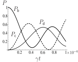
Figure 3: Populations $P_{\sf b}$, $P_{\sf c}$, $P_{\sf d}$ of the three levels b,c,d for $\xi_{12}=\xi$, $\xi_{23}=\xi$, and $\xi_{13}=2\xi$ where $\xi=0.005$, and $\eta=1$. The initial state is $\mathinner{|{\sf b}\rangle}$.

IV.1 Three atoms

To illuminate the detrimental effect of the dipole-dipole interaction on the emission dynamics, the special case of three atoms is considered. For the purposes of this subsection, the linewidths are assumed to coincide with those obtained in the Dicke-limit. This is possible since at $\mathcal{O}(r_{nm})$, $\tilde{\gamma}_{nm}=\tilde{\gamma}/2$ [Eq. (24)]. For one-excitation in three 2LAs, the nonzero off-diagonal elements of $\widehat{H}_{\text{d}}$ are

$$\widehat{H}_{\text{d}}= \;\frac{1}{\sqrt{6}}(\tilde{\Delta}_{13}-\tilde{\Delta}_{23})\mathinner{|{\sf c}\rangle}\mathinner{\langle{\sf d}|}+\frac{2\tilde{\Delta}_{12}-\tilde{\Delta}_{23}-\tilde{\Delta}_{13}}{3\sqrt{2}}\mathinner{|{\sf b}\rangle}\mathinner{\langle{\sf d}|}$$

$$+\frac{\tilde{\Delta}_{23}-\tilde{\Delta}_{13}}{\sqrt{3}}\mathinner{|{\sf b}\rangle}\mathinner{\langle{\sf c}|}+\text{H.c.},$$ (32)

for $\tilde{\Delta}_{nm}=\tilde{\Delta}_{0}+\tilde{\Delta}_{1,nm}$, and $\mathinner{|{\sf b}\rangle}=\tfrac{1}{\sqrt{6}}(-2\mathinner{|{001}\rangle}+\mathinner{|{010}\rangle}+\mathinner{|{100}\rangle})$, $\mathinner{|{\sf c}\rangle}=\frac{1}{\sqrt{2}}(\mathinner{|{010}\rangle}-\mathinner{|{100}\rangle})$, and $\mathinner{|{\sf d}\rangle}=\frac{1}{\sqrt{3}}(\mathinner{|{001}\rangle}+\mathinner{|{010}\rangle}+\mathinner{|{100}\rangle})$. The linewidths of $\mathinner{|{\sf b}\rangle}$, $\mathinner{|{\sf c}\rangle}$, and $\mathinner{|{\sf d}\rangle}$ are $0$, $0$, and $\tfrac{3}{2}\gamma$ respectively—$\mathinner{|{\sf b}\rangle}$ and $\mathinner{|{\sf c}\rangle}$ are subradiant, and $\mathinner{|{\sf d}\rangle}$ is superradiant. Setting $\tilde{\Delta}_{12}=\tilde{\Delta}_{23}=\tilde{\Delta}_{13}=\tilde{\Delta}_{0}$ causes the off-diagonal terms to disappear. So, Dicke emission dynamics are preserved for equal-strength dipole-dipole interactions between the three 2LAs. This can be realized by placing the 2LAs at the vertices of an equilateral triangle.

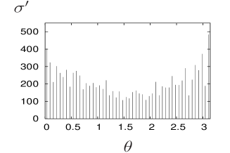
Figure 4: Difference between polar photon counting distributions $\sigma^{\prime}=\sigma_{nd}-\sigma_{wd}$ with $(\sigma_{wd})$ and without $(\sigma_{nd})$ dipole-dipole interactions, for atomic orientation $\eta_{nm}=0$ relative to the dipoles, and separation $r_{nm}=1\times 10^{-10}$m. The distributions are averaged over $100000$ trajectories for $0<t<10^{4}\gamma^{-1}$.

The master equation can be solved using the quantum trajectory method. This unravels the evolution into a sum over records of periods of evolution generated by a non-Hermitian Hamiltonian that are interrupted with stochastic jumps. In the source-mode unravelling detailed in Refs. Carmichael and Kim (2000); Clemens et al. (2003), the only nonzero jump operator in the Dicke basis for $\tilde{\gamma}_{nm}=\tilde{\gamma}$ is

$$\hat{J}=\sqrt{\tilde{\gamma}}\sum_{n=1}^{3}\hat{\sigma}_{n-},$$ (33)

which means that, in the absence of a dipole-dipole interaction, the decay cascade is $\mathinner{|{111}\rangle}\to\tfrac{1}{\sqrt{3}}(\mathinner{|{110}\rangle}+\mathinner{|{101}\rangle}+\mathinner{|{011}\rangle})\to\tfrac{1}{\sqrt{3}}(\mathinner{|{100}\rangle}+\mathinner{|{010}\rangle}+\mathinner{|{001}\rangle})\to\mathinner{|{000}\rangle}$ with probability unity. So, in order for population in the infinite lifetime subradiant states to decay, $\widehat{H}_{\text{d}}$ has to cause population transfer between the subradiant and superradiant states. Fig. 3 shows an example of this population transfer. Population in subradiant state $\mathinner{|{\sf b}\rangle}$ is transferred to the superradiant state $\mathinner{|{\sf d}\rangle}$ on a timescale that is fast compared to $\gamma_{\sf d}^{-1}$.

IV.2 Five atoms

In Ref. Carmichael and Kim (2000) Carmichael and Kim solved the master equation for five atoms. They recovered Dicke superradiance at interatomic separations of $0.025\lambda_{0}$, but with dipole-dipole interactions ignored. They then included dipole-dipole interactions and found that the emission dynamics returned to those expected from individual atoms. Although five atoms is probably too few to support a serious study of directional emission dynamics, the photon counting records of five atoms still show a rich angular dependence. This implies that any influence of the dipole-dipole interaction in the near-Dicke limit on emission direction should still be visible. So, in this section, the directional and temporal emission of five atoms is examined, with the aim of better understanding the effect of the dipole-dipole interaction in the near-Dicke limit.

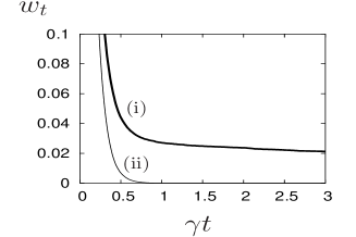
Figure 5: Waiting time distribution of the 5th photon, $w_{t}=\mathinner{\langle{\bar{\Psi}(t)}|}\widehat{B}^{\dagger}(t)\widehat{B}(t)\mathinner{|{\bar{\Psi}(t)}\rangle}$ for $\mathinner{|{\Psi(t=0)}\rangle}$ the normalised state at the time of the 4th photon emission, and $\mathinner{|{\bar{\Psi}(t)}\rangle}$ the unnormalized state at time $t$, (i) including and (ii) excluding the dipole-dipole interaction for five atoms in a linear configuration with interatomic separation $r_{nm}=1\times 10^{-10}$m. The distributions are averaged over $10000$ trajectories.

The unravelling of the superradiance master equation described in Sec. IV.1 accounts for emission time, but does not account for emission direction. In Ref. Carmichael and Kim (2000), the authors proposed an unravelling of the superradiance master equation that yields the directed-detection jump operators

$$\widehat{S}(\theta,\phi)=\sqrt{\gamma D(\theta,\phi)d\Omega}\sum_{n=1}^{N}\text{e}^{-\text{i}k_{0}\vec{R}(\theta,\phi)\cdot\bm{r}_{n}}\widehat{\sigma}_{n-},$$ (34)

which apply when a photon is detected in the far-field (many wavelengths distant) within the element of solid angle $d\Omega$ in direction $\vec{R}(\theta,\phi)$. The dipole radiation pattern $D(\theta,\phi)=\tfrac{3}{8\pi}\{1-[\vec{d}\cdot\vec{R}(\theta,\phi)]^{2}\}$ describes the emission from an isolated atom. The between-jump evolution is described by $\widehat{B}(t)\equiv\text{e}^{-\text{i}\widehat{H}_{B}t}$, where

$$\widehat{H}_{B}= \sum_{n,m=1}^{N}(\tilde{\Delta}^{\perp}_{nm}+\tilde{\Delta}^{\parallel}_{nm})\hat{\sigma}_{n+}\hat{\sigma}_{m-}$$

$$-\frac{\text{i}}{2}\sum^{N}_{n,m=1}\tilde{\gamma}_{nm}\hat{\sigma}_{n+}\hat{\sigma}_{m-}.$$ (35)

Define $\delta n_{\mu}(\theta)$, for $\mu=1,2,\ldots,5$ to be the number of times in an ensemble of quantum trajectories that photon $\mu$ is emitted into solid angle $d\Omega$ around $\theta$, irrespective of the azimuth and time of emission. Then,

$$\sigma(\theta)\equiv\frac{1}{d\Omega}\sum_{\mu=1}^{5}\delta n_{\mu}(\theta),$$ (36)

is the unconditional distribution over polar angle, summed for photons 1 to 5. We calculate $\sigma(\theta)$ for five atoms in a linear configuration at separations of $10^{-10}$m, with and without the dipole-dipole interaction. See Fig. 4. The cut-off implies that the region of validity of the dipole-dipole interaction described by $\tilde{\Delta}$ is bounded below by separations of the order of $a_{0}$. In the calculations, $\tilde{\Delta}(r_{nm}=10^{-10}\text{m})<\tilde{\Delta}_{0}$, and $\tilde{\gamma}_{nm}\approx\tilde{\gamma}/2$. We find that there are less photon emissions when the dipole-dipole interaction is included, implying that the dipole-dipole interaction can transfer population from superradiant states to subradiant states. The angular distribution supports this argument, with the difference in the number of emissions along the axis being greater than the difference at $\theta=\pi/2$.

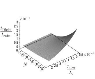
Figure 6: $t_{\text{Dicke}}/t_{\text{rate}}$ for different numbers of atoms, $N$, and separations, $r_{nm}$. The smallest separation was $1.7\times 10^{-4}\lambda_{0}$ and the largest $5.1\times 10^{-4}\lambda_{0}$. For these separations, $\tilde{\gamma}_{nm}\gtrsim 0.99\gamma$, for all $(n,m)$ validating the emission rate approximation.

Fig. 5 shows the waiting time distribution of the fifth photon with and without the dipole-dipole interaction. Without the dipole-dipole interaction, the Dicke model is recovered. However, when the dipole-dipole interactions are included, population is transfered from subradiant states to super-radiant states, leading to the extended tail seen in Fig. 5.

IV.3 $N$ atoms

For many atom systems it is not possible to solve the master equation exactly—sensible approximations are required for anything more than a few atoms. However, it is possible to estimate the relevant timescales for Dicke dynamics in the near-Dicke limit. Fig. 3 gives some indication of the relevant timescales. For small times, Dicke dynamics are preserved. This can be quantified as follows. The unitary evolution of an arbitrary $N$-atom state, $\mathinner{|{\Psi}\rangle}$ is

$$\mathinner{|{\Psi(t)}\rangle}=\text{e}^{-\text{i}\widehat{H}_{\text{d}}t}\mathinner{|{\Psi(0)}\rangle},$$ (37)

with $\widehat{H}_{\text{d}}$ of Eq. (26). So, the (shortest) timescale for Dicke dynamics in the near-Dicke limit is

$$t_{\text{Dicke}}\sim||\widehat{H}_{\text{d}}||^{-1},$$ (38)

where $||\cdot||$ denotes maximum eigenvalue. Typical values for $\tilde{\Delta}^{\parallel}_{nm}+\tilde{\Delta}^{\perp}_{nm}$ in the near-Dicke limit are $\sim 10^{8}\gamma_{0}$. Eq. (38) is an estimate only, and implicitly assumes that the dipole-dipole interaction matrix and the spontaneous emission matrix are not simultaneously diagonalizable. Because of the spatial dependence of $\widehat{H}_{\text{d}}$, this is always true for any system consisting of more than four atoms.

As well as estimating an upper limit on the timescale for Dicke dynamics, it is possible to estimate the superradiant emission rate for separations ${\cal O}(r)$. We neglect the ${\cal O}(r^{2})$ corrections to $\tilde{\gamma}_{nm}$ and $\tilde{\Delta}^{\parallel}_{nm}+\tilde{\Delta}^{\perp}_{nm}$. At (finite) separations of ${\cal O}(r)$, the dipole-dipole interaction and collective spontaneous emission rate can be described by Eqs. (22), (23) and (24). The collective decay rates then correspond to those predicted by Dicke—the eigenspectrum of $(\tilde{\gamma}_{nm})$ is the same as that obtained in the Dicke limit. So, we can approximate the maximum emission rate as

$$t_{\text{rate}}=\left\{\frac{\tilde{\gamma}}{2}N\left(\frac{1}{2}N+1\right)\right\}^{-1},$$ (39)

which occurs for $\tfrac{1}{2}N$ excited atoms in an $N$ atom system.

To estimate the competing timescales, we take the ratio $t_{\text{Dicke}}/t_{\text{rate}}$. We assume that $t_{\text{Dicke}}$ is of the order of the quickest (population) mixing rate for $N$ excited atoms, so the ratio $t_{\text{Dicke}}/t_{\text{rate}}$ compares the fastest mixing timescale (for systems of more than four atoms) with the superradiant decay timescale.

Fig. 6 shows the effect of the interatomic separation and the number of atoms on the emission rate. As the number of atoms increases, the superradiant emission rate begins to dominate over the mixing induced by the dipole-dipole interaction. We emphasize that our results are only valid for atomic systems in the near-Dicke limit, i.e., when the spatial extent of the atomic system ensures that Eqs. (22), (23), and (24) are satisfied for all atoms.

V Conclusion

We renormalized the divergent superradiance master equation in both the electric-dipole and minimal-coupling pictures. The propagating and nonpropagating parts of the dipole-dipole interaction were accounted for separately, and two values for the relevant cut-offs were proposed. Then, it was shown explicitly for small numbers of atoms that the dipole-dipole interaction causes population transfer between the super- and subradiant Dicke states, resulting in increased emission times. This was confirmed by the directional emission counting distribution for five atoms that showed less emissions along the interatomic axis. It was then shown for large numbers of atoms in the near-Dicke limit that as the number of atoms increases, the effect of the dipole-dipole interaction on the emission dynamics for 2LAs in a linear arrangement is reduced.

VI Acknowledgments

This project has been funded by iCORE, CIFAR, NSERC, CQCT, and Macquarie University. One of the authors (P.G.B.) acknowledges support and hospitality during his extended stay at IQIS at the University of Calgary. We thank Sir Peter Knight for discussions and Martin Kiffner for helpful comments on the manuscript.

Appendix A Derivation of the regularized master equation in minimal coupling

In order to derive the master equation of the atomic system in minimal-coupling, the matrix elements of the dipole operator ${\bm{d}}\equiv\langle e|\hat{{\bm{d}}}|g\rangle$ are related to the matrix elements of the electronic momentum operator by

$${\bm{p}}\equiv\langle e|\hat{{\bm{p}}}|g\rangle=\frac{\text{i}\,m}{\hbar q}({\cal E}_{e}-{\cal E}_{g})\langle e|\hat{{\bm{d}}}|g\rangle\;,$$ (40)

with $m$ the electron’s mass, $q$ its charge, and ${\cal E}_{i}$ the atomic energy levels (see, eg., p. 74 of Ref. Sakurai (1976)). In the interaction picture with respect to the system Hamiltonian (1) the momentum operator becomes

$$\hat{\bm{p}}_{n}(-\tau)=\hat{\sigma}_{n\textrm{\tiny{+}}}\text{e}^{-\text{i}\tau\omega_{0}}\bm{p}+\hat{\sigma}_{n\textrm{\tiny{-}}}\text{e}^{\text{i}\tau\omega_{0}}\bm{p}^{*},$$ (41)

where $\hat{{\bm{p}}}_{n}(\tau)=U^{\dagger}_{\text{s}}\hat{{\bm{p}}}_{n}U_{\text{s}}$ and $U_{\text{s}}=\text{exp}(-\text{i}\tau\widehat{H}_{\text{s}}/\hbar)$. For convenience, $\hat{{\bm{p}}}_{n}(0)=\hat{{\bm{p}}}_{n}$. The interaction Hamiltonian describes a minimal-coupling between the atom and electric field

$$\widehat{H}_{\text{int}}=-\frac{q}{m}\sum_{n=1}^{N}\hat{\bm{p}}_{n}\cdot\widehat{\bm{A}}(\bm{r}_{n})+\frac{q^{2}}{2m}\sum_{n=1}^{N}\widehat{\bm{A}}(\bm{r}_{n})^{2},$$ (42)

where $\widehat{\bm{A}}(\bm{r}_{n})$ is the Hermitian operator of the vector potential. The full Hamiltonian in the Coulomb gauge, neglecting the free, transverse electric-field and the free Hamiltonian of atom $n$,

$$\widehat{H}_{\text{mc}}=\widehat{H}_{\text{s}}+\widehat{H}_{\text{int}}+\widehat{H}_{\text{c}}\;,$$ (43)

also includes a static interaction described by Power and Zienau (1957); Friedberg et al. (1973); Agarwal (1974)

$$\widehat{H}_{\text{c}}=\sum_{n,m=1}^{N}\hbar\Delta^{\parallel}_{nm}\hat{\sigma}_{n+}\hat{\sigma}_{m-},$$ (44)

for $\Delta^{\parallel}_{nm}$ of Eq. (5). The electrostatic dipole-dipole interaction describes a nonretarded interaction that is not mediated by a transverse propagator Power and Zienau (1957, 1959); Agarwal (1974). The term proportional to $\widehat{{\bm{A}}}^{2}$ can be omitted because in the dipole approximation it contributes the same energy to every atomic state Milonni (1994). This term includes the self-energy of the electric dipole, which also does not contribute to relative energy shifts Cohen-Tannoudji et al. (1989). So,

$$\widehat{H}_{\text{int}}=-\frac{q}{m}\sum_{n=1}^{N}\hat{\bm{p}}_{n}\cdot\widehat{\bm{A}}(\bm{r}_{n})=-\frac{q}{m}\sum_{i=1}^{3}\sum_{n=1}^{N}\hat{p}_{n,i}\widehat{A}_{i}(\bm{r}_{n}),$$ (45)

where the subscript $i$ labels the $i^{\text{th}}$ vector component. In the Born-Markov approximation, the time evolution of the reduced density operator for identical 2LAs $n$ and $m$ is given by

$$\dot{\rho}= -\frac{\text{i}}{\hbar}[\widehat{H}_{\text{s}}+\widehat{H}_{\text{c}},\rho]$$

$$-\frac{q^{2}}{m^{2}\hbar^{2}}\int_{0}^{\infty}\text{d}\tau\sum_{i,j=1}^{3}\sum_{n,m=1}^{N}\big{(}\langle\widehat{A}_{i}(\tau,\bm{r}_{n})\widehat{A}_{j}(0,\bm{r}_{m})\rangle$$

$$\times[\hat{p}_{n,i},\hat{p}_{m,j}(-\tau)\rho]+\langle\widehat{A}_{j}(0,\bm{r}_{m})\widehat{A}_{i}(\tau,\bm{r}_{n})\rangle$$

$$\times[\rho\hat{p}_{m,j}(-\tau),\hat{p}_{n,i}]\big{)},$$ (46)

for $\widehat{A}(\tau)=U^{\dagger}_{\text{R}}\widehat{A}U_{\text{R}}$ for $U_{\text{R}}=\text{exp}(-\text{i}\tau\widehat{H}_{\text{R}})$ the reservoir operators in the interaction picture. The reservoir Hamiltonian $\widehat{H}_{R}$ is time independent, so $\langle\widehat{A}_{i}(\tau,\bm{r}_{n})\widehat{A}_{j}(0,\bm{r}_{m})\rangle=\langle\widehat{A}_{j}(0,\bm{r}_{m})\widehat{A}_{i}(-\tau,\bm{r}_{n})\rangle$. Making the rotating-wave approximation and assuming that the reservoir is initially in the vacuum state, the master equation can be written

$$\dot{\rho}= -\frac{\text{i}}{\hbar}[\widehat{H}_{\text{s}}+\widehat{H}_{\text{c}},\rho]+\sum_{n=1}^{N}F^{-}_{nn}[\hat{\sigma}_{nz},\rho]$$

$$-\sum_{n,m=1}^{N}I_{nm}^{+}[\hat{\sigma}_{n+},\hat{\sigma}_{m-}\rho]+(I_{mn}^{+})^{*}[\rho\hat{\sigma}_{m+},\hat{\sigma}_{n-}],$$ (47)

where $I_{nm}^{\pm}\equiv F_{nm}^{+}\pm F_{nm}^{-}$ for

$$F_{nm}^{\pm}\equiv \sum_{i,j=1}^{3}\frac{q^{2}p_{i}p^{*}_{j}}{m^{2}\hbar^{2}}\lim_{\epsilon\rightarrow 0}\int_{0}^{\infty}\text{d}\tau\times\mathinner{\langle{0}|}\widehat{A}_{i}^{(+)}(\tau,\bm{r}_{n})$$

$$\times\widehat{A}_{j}^{(-)}(0,\bm{r}_{m})\mathinner{|{0}\rangle}\text{e}^{\pm\text{i}\omega_{0}\tau-\epsilon\tau}$$

$$= \sum_{i,j=1}^{3}\frac{\omega_{0}^{2}d_{i}d_{j}^{*}}{\hbar^{2}}\lim_{\epsilon\rightarrow 0}\int_{0}^{\infty}\text{d}\tau\mathinner{\langle{0}|}\widehat{A}_{i}^{(+)}(\tau,\bm{r}_{n})$$

$$\times\widehat{A}_{j}^{(-)}(0,\bm{r}_{m})\mathinner{|{0}\rangle}\text{e}^{\pm\text{i}\omega_{0}\tau-\epsilon\tau},$$ (48)

in which the infinitesimal number $\epsilon>0$ has been added to ensure the correct analytical properties in the complex plane. In the Coulomb gauge, the electric field is separated into propagating (transverse) and nonpropagating (longitudinal) parts. Here, the superscript ‘$\perp$’ labels transverse in order to distinguish between the propagating (transverse) and static (longitudinal) dipole-dipole interaction. The correlation function is

$$\langle\widehat{A}_{i}^{(+)}(\tau,\bm{r}_{n}) \widehat{A}_{j}^{(-)}(0,\bm{r}_{m})\rangle=\frac{\hbar}{4\pi^{2}\varepsilon_{0}c}\int_{0}^{\infty}\text{d}k\;k\,$$

$$\times\text{e}^{-\text{i}\omega_{k}\tau}(\alpha(kr_{nm})+\vec{r}_{nm,i}\vec{r}_{nm,j}\beta(kr_{nm})),$$ (49)

where the frequency of the electric field $\omega_{k}=ck$ for $k=|{\bm{k}}|$, and $\alpha$ and $\beta$ given in Eq. (6) and (7), respectively. We use an arrow to denote a unit vector. For instance, $\vec{r}_{nm}$ corresponds to the unit vector $\vec{r}_{nm}=\bm{r}_{nm}/r_{nm}$ in the direction of the vector $\bm{r}_{nm}\equiv\bm{r}_{n}-\bm{r}_{m}$. In order to calculate explicit expressions for $\gamma_{nm}$ and $\Delta_{nm}$, $F_{nm}^{\pm}$ is written as

$$F_{nm}^{\pm} =-\text{i}\frac{\omega_{0}^{2}|{\bm{d}}|^{2}}{4\pi^{2}\varepsilon_{0}\hbar c}\lim_{\epsilon\rightarrow 0}\int_{0}^{\infty}\text{d}k\;k\,\frac{\alpha(kr_{nm})+\eta_{nm}\beta(kr_{nm})}{\omega_{k}\mp\omega_{0}-\text{i}\epsilon},$$

$$=\frac{3\gamma}{4\pi\text{i}k_{0}}\lim_{\epsilon\rightarrow 0}\int_{0}^{\infty}\text{d}k\;k\,\frac{\alpha(kr_{nm})+\eta_{nm}\beta(kr_{nm})}{k\mp k_{0}-\text{i}\epsilon}\;,$$ (50)

So, the quantity $I_{nm}^{+}$ can be written

$$I_{nm}^{+}=\frac{3\gamma}{4\pi\text{i}k_{0}}\lim_{\epsilon\to 0}\int_{-\infty}^{\infty}\text{d}k\;k\,\frac{\alpha(kr_{nm})+\eta_{nm}\beta(kr_{nm})}{k-k_{0}-\text{i}\epsilon}\;,$$ (51)

which can be integrated using the residue theorem. It has a pole at $k_{0}+\text{i}\epsilon$, and so is integrated taking care to separate terms proportional to $\exp(\text{i}kr_{nm})$, for which the contour has to be closed in the upper half plane, from those terms proportional to $\exp(-\text{i}kr_{nm})$. While the total expression has no pole at $k=0$, each of these terms diverges at this point and the corresponding residue has to be taken into account. Eq. (51) then leads to $\gamma_{nm}\equiv\Re(I_{nm}^{+})$ given in Eq. (3) and $\Delta_{nm}^{\perp}\equiv\Im(I_{nm}^{+})$ given in Eq. (4). The collective emission and level shift coefficients are identified as $\gamma_{nm}$ and $\Delta_{nm}^{\perp}+\Delta_{nm}^{\parallel}$, respectively. The last term in Eq. (4), which arises from the pole at $k=0$, cancels with the static part of the full Hamiltonian quoted in Eq.(44) Power and Zienau (1957, 1959); Agarwal (1974); Friedberg et al. (1973). So, the master equation is written

$$\dot{\rho}= -\frac{\text{i}}{\hbar}[\widehat{H}_{\text{s}},\rho]-\text{i}\sum_{n,m=1}^{N}(\Delta^{\perp}_{nm}+\Delta^{\parallel}_{nm})[\hat{\sigma}_{n+}\hat{\sigma}_{m-},\rho]$$

$$+\sum_{n,m=1}^{N}{\gamma}_{nm}(2\hat{\sigma}_{m-}\rho\hat{\sigma}_{n+}-\hat{\sigma}_{n+}\hat{\sigma}_{m-}\rho-\rho\hat{\sigma}_{n+}\hat{\sigma}_{m-}).$$ (52)

The single-atom level shift obtained from the master equation for a single-atom

$$\dot{\rho}= -\frac{\text{i}}{\hbar}[\widehat{H}_{\text{s}}+\widehat{H}_{\text{c}},\rho]-\frac{\text{i}}{2}\Im\{I_{nn}^{-}\}[\hat{\sigma}_{z},\rho]$$

$$-\Re\{I_{nn}^{+}\}(\hat{\sigma}_{+}\hat{\sigma}_{-}\rho+\rho\hat{\sigma}_{+}\hat{\sigma}_{-}-2\hat{\sigma}_{-}\rho\hat{\sigma}_{+}),$$ (53)

is equal to the imaginary part of $I_{nn}^{-}$

$$\Delta_{\text{Lamb}}^{\text{(2-lev)}} \equiv\Im\{I_{nn}^{-}\}$$

$$=\frac{\gamma}{2\pi k_{0}}\left(\mathcal{P}\int_{0}^{\infty}\text{d}k\frac{k}{k-k_{0}}-\mathcal{P}\int_{0}^{\infty}\text{d}k\frac{k}{k+k_{0}}\right),$$

$$=\frac{\gamma}{2\pi}\mathcal{P}\int_{0}^{\infty}\text{d}k\left(\frac{1}{k-k_{0}}+\frac{1}{k+k_{0}}\right),$$ (54)

where the limit $\xi_{nm}\to 0$ has been taken in $F^{\pm}_{nm}$, and where $\mathcal{P}$ denotes principal value. This normally is absorbed into $\widehat{H}_{s}$ by appropriate redefinition of the eigenfrequency $\omega_{0}$. It is connected with the single-atom Lamb shift Bethe (1947), but because of the two-level approximation it only includes the energy shift generated by the coupling between the two basis states.

Regularization

The divergence of both Eq. (51) and Eq. (A) can be removed using a regularization factor $\Lambda_{\perp}^{2}/(\Lambda_{\perp}^{2}+k^{2})$. For the imaginary part of the single-atom quantity, this gives

$$\Delta_{\text{Lamb}}^{\text{(2-lev)}} =\frac{\gamma}{2\pi}\mathcal{P}\int_{0}^{\infty}\text{d}k\left(\frac{1}{k-k_{0}}+\frac{1}{k+k_{0}}\right)\frac{\Lambda_{\perp}^{2}}{k^{2}+\Lambda_{\perp}^{2}}.$$ (55)

This integral becomes

$$\Delta_{\text{Lamb}}^{\text{(2-lev)}}=\frac{\tilde{\gamma}}{\pi}\ln\left(\frac{\Lambda_{\perp}}{k_{0}}\right).$$ (56)

The multi-atom quantity $I_{nm}^{+}$ is regularized in a similar way

$$\tilde{I}_{nm}^{+}=\frac{3\gamma}{4\pi\text{i}k_{0}}\lim_{\epsilon\to 0}\int_{-\infty}^{\infty} \text{d}k\;k\,\frac{\alpha(kr_{nm})+\eta_{nm}\beta(kr_{nm})}{k-k_{0}-\text{i}\epsilon}$$

$$\times\frac{\Lambda_{\perp}^{2}}{\Lambda_{\perp}^{2}+k^{2}}.$$ (57)

The small $r_{nm}$ behaviour is now moderated. By implication, the details of the interaction region are not of specific interest de Vries et al. (1998). We remark that this regularization procedure is not unique. Eq. (A) has poles at $k_{0}+\text{i}\epsilon$ and $\pm\text{i}\Lambda_{\perp}$, and so is integrated using the residue theorem. Using $\tilde{\gamma}$ of Eq. (11) and calculating the integral in Eq. (A) results in Eqs. (8) and (9), where we defined $\tilde{\gamma}_{nm}\equiv\Re(\tilde{I}_{nm}^{+})$ and $\tilde{\Delta}^{\perp}_{nm}\equiv\Im(\tilde{I}_{nm}^{+})$.

Taking $\Lambda_{\perp}\to\infty$ recovers Eq. (3) and (4). The dipole-dipole interaction $\tilde{\Delta}_{nm}^{\perp}$ is now regularized, with the limiting values given by

$$\lim_{r_{nm}\to 0}\tilde{\Delta}^{\perp}_{nm}=-\frac{\tilde{\gamma}\Lambda_{\perp}}{2k_{0}},$$ (58)

and

$$\lim_{r_{nm}\to 0}\tilde{\gamma}_{nm}=\frac{\tilde{\gamma}}{2}.$$ (59)

Note that if $\Lambda_{\perp}\gg k_{0}$, $\tilde{\gamma}\simeq\gamma$, and also that $\lim_{r_{nm}\to 0}\gamma_{nm}=\gamma/2$, where $\gamma_{nm}$ is defined in Eq. (3).

For $\Lambda_{\perp}\to\infty$, the final term in Eq. (9) cancels the static dipole-dipole interaction to give Eq. (A). However, subtracting this term as before changes the properties of $\tilde{\Delta}_{nm}^{\perp}$ such that it once again diverges as $r_{nm}\to 0$. So, in order to maintain the analytic properties of $\tilde{I}_{nm}^{+}$ in the limit $r_{nm}\to 0$, it is necessary to retain the final term in $\tilde{\Delta}_{nm}^{\perp}$. The problem is then that the static, divergent, dipole-dipole interaction $\widehat{H}_{c}$ of Eq. (44) remains in the original Hamiltonian. In order to account for the divergence, we regularize $\widehat{H}_{c}$ as follows. First, notice that Cohen-Tannoudji et al. (1989)

$$\Delta^{\parallel}_{nm}=\frac{|\bm{d}|^{2}}{\hbar\varepsilon_{0}}\left(\vec{d}_{n}\cdot G(k,\bm{r})\cdot\vec{d}_{m}\right),$$ (60)

where the Green’s function $G(k,\bm{r})$ is

$$G_{ij}(k,\bm{r})=\int\frac{\text{d}^{3}k}{(2\pi)^{3}}\vec{k}_{i}\vec{k}_{j}\text{e}^{\text{i}\bm{k}\cdot(\bm{r}_{n}-\bm{r}_{m})}.$$ (61)

This can be regularized in a similar way to before:

$$\tilde{G}_{ij}(k,\bm{r})=\int\frac{\text{d}^{3}k}{(2\pi)^{3}}\vec{k}_{i}\vec{k}_{j}\text{e}^{\text{i}\bm{k}\cdot(\bm{r}_{n}-\bm{r}_{m})}\frac{\Lambda^{4}_{\parallel}}{k^{4}+\Lambda^{4}_{\parallel}}.$$ (62)

The regularization parameter is raised to the fourth power in order to account for the $r^{3}$ divergence of the static interaction. Eq. (62) can be written

$$\tilde{\Delta}^{\parallel}_{nm}= \frac{|\bm{d}|^{2}}{2\hbar\pi^{2}\varepsilon_{0}}\int_{0}^{\infty}k^{2}\text{d}k\Bigg{\{}\frac{\sin\xi_{nm}}{\xi_{nm}^{3}}-\frac{\cos\xi_{nm}}{\xi_{nm}^{2}}$$

$$+\eta_{nm}\left[\frac{3\cos\xi_{nm}}{\xi_{nm}^{2}}-\frac{3\sin\xi_{nm}}{\xi_{nm}^{3}}+\frac{\sin\xi_{nm}}{\xi_{nm}}\right]\Bigg{\}}$$

$$\times\frac{\Lambda^{4}_{\parallel}}{k^{4}+\Lambda^{4}_{\parallel}}.$$ (63)

Evaluating this expression gives Eq. (II). Again, taking $\Lambda_{\parallel}\to\infty$ recovers $\Delta^{\parallel}_{nm}$. The static interaction is now regularized with limiting value given by

$$\lim_{r_{nm}\to 0}\tilde{\Delta}^{\parallel}_{nm}=\frac{\gamma\Lambda_{\parallel}^{3}}{4\sqrt{2}k_{0}^{3}}.$$ (64)

Hence, the fully regularized master equation is given by Eq. (II), where the parameters are given by $\tilde{\gamma}_{nm}$ of Eq. (8), $\tilde{\Delta}^{\perp}_{nm}$ of Eq. (9), and $\tilde{\Delta}^{\parallel}_{nm}$ of Eq. (II). In the regime where regularization matters, there is no longer a complete cancellation of $\widehat{H}_{c}$. As the separation of the 2LAs increases, Eq. (II) approaches Eq. (A). The regularization has smeared the zero-spatial extent of the point-dipoles. It remains to show the equivalence with the electric-dipole Hamiltonian and to propose a value for $\Lambda_{\parallel}$ and $\Lambda_{\perp}$. Here, we note a few important remarks.

First, as is normal in the Coulomb gauge, the electric field is split into a longitudinal and a transverse field. The retarded nature of the electromagnetic field results from an exact compensation between two instantaneous parts derived from the Coulomb field and the transverse field respectively (see Eq. (4)). With the cut-offs applied, this cancellation no longer occurs in the near-Dicke limit. The dipole-dipole interaction at small separations includes, but does not consist entirely of, a contact term. This is in contrast to the result, stated in Eq. (44), derived in Ref. Gross and Haroche (1982). We conjecture that the origin of non-retarded terms lies in the choice of different cut-off parameters for transverse and longitudinal fields, which explicitly breaks the covariance of Maxwell’s theory and hence can violate causality. The ultimate reason for this different treatment is that we work in Coulomb gauge, which is the standard choice to describe atom-light interactions but which is not covariant. It would probably be possible to remove the non-retarded terms by using a covariant description of the atom-light coupling, but this effort would not be justified because in the near-Dicke limit retardation effects can safely be ignored.

Second, the assumptions behind our model imply that relativistic effects, such as vacuum polarization or relativistic recoil, are not included. This approximation is justified as long as the resonance energy $\hbar\omega_{0}$ of the two-level systems is much smaller than the rest energy $mc^{2}$ of the electron. Relativistic effects would lead to modifications of our treatment on a length scale of the order of the electron’s Compton wavelength $2\pi\hbar/(mc)$.

Appendix B Derivation of the regularized master equation in electric-dipole coupling

The Lindblad master equation derived previously describes the evolution of a collection of minimally coupled 2LAs. We would expect the result to be the same using the multipolar Hamiltonian for two reasons. First, Eqs. (3) and (4) are equivalent to the more commonly used electric-dipole master equation Belavkin et al. (1969); Lehmberg (1970a); Agarwal (1970); Carmichael and Kim (2000); Clemens et al. (2003). Second, the full minimal-coupling Hamiltonian is unitarily equivalent to the full multipolar Hamiltonian. We follow the same method as Sec. A, but take care to distinguish the differences. Transforming to the interaction picture gives

$$\hat{\bm{d}}_{n}(-\tau)=\widehat{\sigma}_{n\textrm{\tiny{+}}}\text{e}^{-\text{i}\tau\omega_{0}}\bm{d}+\widehat{\sigma}_{n\textrm{\tiny{-}}}\text{e}^{\text{i}\tau\omega_{0}}\bm{d}^{*},$$ (65)

where $\hat{\bm{d}}_{n}(\tau)=U^{\dagger}_{\text{s}}\hat{\bm{d}}_{n}U_{\text{s}}$. For convenience, $\hat{{\bm{d}}}_{n}(0)=\hat{{\bm{d}}}_{n}$. The interaction Hamiltonian describes an electric-dipole coupling between the atom and electric field

$$\widehat{H}_{\text{int}}=-\sum_{n=1}^{N}\hat{\bm{d}}_{n}\cdot\widehat{\bm{E}}(\bm{r}_{n})=-\sum_{i=1}^{3}\sum_{n=1}^{N}\hat{d}_{n,i}\widehat{E}_{i}(\bm{r}_{n}).$$ (66)

Using the multipolar Hamiltonian, an extra term

$$\widehat{H}_{\text{self}}=\frac{1}{2\varepsilon_{0}}\sum_{n\neq m=1}^{N}\int\text{d}^{3}\bm{r}\widehat{\bm{P}}_{n}(\bm{r})\cdot\widehat{\bm{P}}_{m}(\bm{r}),$$ (67)

where, in the electric-dipole approximation,

$$\widehat{\bm{P}}_{n}(\bm{r})=\hat{\bm{d}}_{n}\delta(\bm{r}-\bm{r}_{n})$$ (68)

describing atomic self-energies and contact interactions is present. These terms result from applying the Power-Zienau-Woolley transformation

$$\mathcal{U}=\text{exp}\left[-\frac{\text{i}}{\hbar}\sum_{n=1}^{N}\int\text{d}^{3}\bm{r}\widehat{\bm{P}}_{n}(\bm{r})\cdot\widehat{\bm{A}}(\bm{r}_{n})\right]$$ (69)

to Eq. (43). We apply the transformation as $\mathcal{U}\widehat{H}_{\text{mc}}\mathcal{U}^{\dagger}$, so $\widehat{\bm{E}}$ represents the electric-field. See Ref. Cohen-Tannoudji et al. (1989) for an introduction to the Power-Zienau-Woolley transformation, and Ref. Davidovich for a deeper analysis that refutes some of the results in Ref. Power and Zienau (1957) and highlights the importance of the order with which one applies the transformation. We assume that any terms that refer to self-energies of a single atom are renormalized into $\widehat{H}_{\text{s}}$. Thus, the full electric-dipole Hamiltonian is

$$\widehat{H}_{\text{ed}}=\widehat{H}_{\text{s}}+\widehat{H}_{\text{int}}+\widehat{H}_{\text{self}}.$$ (70)

In the Born-Markov and electric-dipole approximation, the time evolution of the reduced density operator for atoms $n$ and $m$ is given by

$$\dot{\rho}= -\frac{\text{i}}{\hbar}[\widehat{H}_{\text{s}}+\widehat{H}_{\text{self}},\rho]$$

$$-\frac{1}{\hbar^{2}}\int_{0}^{\infty}\text{d}\tau\sum_{i,j=1}^{3}\sum_{n,m=1}^{N}\big{(}\langle\widehat{E}_{i}(\tau,\bm{r}_{n})\widehat{E}_{j}(0,\bm{r}_{m})\rangle$$

$$\times[\hat{d}_{n,i},\hat{d}_{m,j}(-\tau)\rho]$$

$$+\langle\widehat{E}_{j}(0,\bm{r}_{m})\widehat{E}_{i}(\tau,\bm{r}_{n})\rangle[\rho\hat{d}_{m,j}(-\tau),\hat{d}_{n,i}]\big{)},$$ (71)

for $\widehat{E}(\tau)=U^{\dagger}_{\text{R}}\widehat{E}U_{\text{R}}$ for $U_{\text{R}}=\text{exp}(-\text{i}\tau\widehat{H}_{\text{R}})$ the reservoir operators in the interaction picture. The reservoir Hamiltonian $H_{R}$ is time independent, so $\langle\widehat{E}_{i}(\tau,\bm{r}_{n})\widehat{E}_{j}(0,\bm{r}_{m})\rangle=\langle\widehat{E}_{j}(0,\bm{r}_{m})\widehat{E}_{i}(-\tau,\bm{r}_{n})\rangle$. Following the notation of Sec. A, $F_{nm}^{\pm}$ is defined as

$$F_{nm}^{\pm}\equiv \sum_{i,j=1}^{3}\frac{d_{i}d_{j}^{*}}{\hbar^{2}}\lim_{\epsilon\rightarrow 0}\int_{0}^{\infty}\text{d}\tau\mathinner{\langle{0}|}\widehat{E}_{i}^{(+)}(\tau,\bm{r}_{n})$$

$$\times\widehat{E}_{j}^{(-)}(0,\bm{r}_{m})\mathinner{|{0}\rangle}\text{e}^{\pm\text{i}\omega_{0}\tau-\epsilon\tau}$$ (72)

and the correlation function is

$$\langle\widehat{E}_{i}^{(+)}(\tau,\bm{r}_{n}) \widehat{E}_{j}^{(-)}(0,\bm{r}_{m})\rangle=\frac{\hbar c}{4\pi^{2}\varepsilon_{0}}\int_{0}^{\infty}\text{d}k\;k^{3}\,$$

$$\times\text{e}^{-\text{i}\omega_{k}\tau}(\alpha(\xi_{nm})+\vec{r}_{nm,i}\vec{r}_{nm,j}\beta(\xi_{nm})).$$ (73)

This is not equal to, but has the same fundamental properties as Eq. (A) which means the master equation can be written in the form

$$\dot{\rho}= -\frac{\text{i}}{\hbar}[\widehat{H}_{\text{s}}+\widehat{H}_{\text{self}},\rho]+\sum_{n=1}^{N}F^{-}_{nn}[\hat{\sigma}_{nz},\rho]$$

$$-\sum_{n,m=1}^{N}I_{nm}^{+}[\hat{\sigma}_{n+},\hat{\sigma}_{m-}\rho]+(I_{mn}^{+})^{*}[\rho\hat{\sigma}_{m+},\hat{\sigma}_{n-}],$$ (74)

where $I_{nm}^{\pm}\equiv F_{nm}^{+}\pm F_{nm}^{-}$. So, as in Sec. A the collective emission coefficient and the level shift operator are identified as $\gamma_{nm}\equiv\Re(I_{nm}^{+})$ and $\Delta_{nm}\equiv\Im(I_{nm}^{+})$ respectively. The non-regularized quantity $F_{nm}^{\pm}$ is written as

$$F_{nm}^{\pm}=\frac{|\bm{d}|^{2}}{4\pi^{2}\text{i}\varepsilon_{0}\hbar}\lim_{\epsilon\to 0}\int_{0}^{\infty}\text{d}k\;k^{3}\frac{\alpha(\xi_{nm})+\eta_{nm}\beta(\xi_{nm})}{k\mp k_{0}-\text{i}\epsilon}.$$ (75)

The crucial difference between Eq. (A) and Eq. (75) is the order of the divergence. Here, it is proportional to $k^{3}$ but in minimal-coupling it is proportional to $k$. If this divergence is not accounted for and the regularization proceeds directly from here, the two regularized answers using the minimal-coupling and the electric-dipole Hamiltonians will be different.

Equivalence with minimal-coupling

In order to account for the difference in the divergence, the self-energy given by Eq. (67) is examined more closely. Calculating this integral sheds light on the origin of the higher divergence of Eq. (75): in the electric-dipole picture the self-energies of the atomic dipoles have been implicitly included. These same energies form part of the $\widehat{{\bm{A}}}^{2}$ term in minimal-coupling. So, making the rotating wave approximation and using the commutation relation $[\hat{\sigma}_{n-},\hat{\sigma}_{m+}]=0\;\forall\;n\neq m$, the self-energy contribution is

$$\widehat{H}_{\text{self}}=\sum_{i,j=1}^{3}\frac{d_{i}\,\delta_{ij}\,d_{j}^{*}}{\varepsilon_{0}}\sum_{n\neq m=1}^{N}\hat{\sigma}_{n+}\hat{\sigma}_{m-}\delta(\bm{r}_{n}-\bm{r}_{m}),$$ (76)

which can be decomposed into longitudinal and transverse parts

$$\widehat{H}_{\text{self}}= \sum_{i,j=1}^{3}\frac{d_{i}d_{j}^{*}}{\varepsilon_{0}}\sum_{n\neq m=1}^{N}\hat{\sigma}_{n+}\hat{\sigma}_{m-}$$

$$\times\bigg{\{}\delta^{\perp}_{ij}(\bm{r}_{n}-\bm{r}_{m})+\delta^{\parallel}_{ij}(\bm{r}_{n}-\bm{r}_{m})\bigg{\}}.$$ (77)

The transverse delta function, which is proportional to the commutator of the vector potential and the transverse electric field, is defined by

$$\delta^{\perp}_{ij}(\bm{r}_{n}-\bm{r}_{m}) =\int\frac{\text{d}^{3}k}{(2\pi)^{3}}\left(\delta_{ij}-\frac{{k}_{i}{k}_{j}}{k^{2}}\right)\text{e}^{\text{i}\bm{k}\cdot(\bm{r}_{n}-\bm{r}_{m})}$$

$$=\frac{1}{2\pi^{2}}\int_{0}^{\infty}\text{d}k\;k^{2}\,\{\alpha(\xi_{nm})\,\delta_{ij}$$

$$\hskip 56.9055pt+\vec{r}_{nm,i}\,\vec{r}_{nm,j}\,\beta(\xi_{nm})\}$$ (78)

for $\alpha(\xi_{nm})$ and $\beta(\xi_{nm})$ defined in Eqs. (6) and (7), respectively. The longitudinal delta function is defined as

$$\delta^{\parallel}_{ij}(\bm{r}_{n}-\bm{r}_{m})=\int\frac{\text{d}^{3}k}{(2\pi)^{3}}\frac{k_{i}k_{j}}{k^{2}}\text{e}^{\text{i}\bm{k}\cdot(\bm{r}_{n}-\bm{r}_{m})}\;,$$ (79)

which is the same expression as in Eq. (61). The transverse part of $\widehat{H}_{\text{self}}$ becomes

$$\widehat{H}^{\perp}_{\text{self}}= \frac{|\bm{d}|^{2}}{2\pi^{2}\varepsilon_{0}}\sum_{n\neq m=1}^{N}\hat{\sigma}_{n+}\hat{\sigma}_{m-}\int_{0}^{\infty}\text{d}k\;k^{2}\{\alpha(\xi_{nm})$$

$$+\eta_{nm}\beta(\xi_{nm})\}$$ (80)

for $\eta_{nm}\equiv(\vec{d}\cdot\vec{r}_{nm})^{2}$. Writing $I_{nm}^{+}$ in electric-dipole coupling as

$$I_{nm}^{+} =\frac{|\bm{d}|^{2}}{4\pi^{2}\text{i}\varepsilon_{0}\hbar}\int_{-\infty}^{\infty}\text{d}k\;k^{3}\frac{\alpha(\xi_{nm})+\eta_{nm}\beta(\xi_{nm})}{k-k_{0}-\text{i}\epsilon}$$

$$=\frac{|\bm{d}|^{2}}{4\pi^{2}\text{i}\varepsilon_{0}\hbar}\bigg{\{}\int_{0}^{\infty}\text{d}k\;2k^{2}\{\alpha(\xi_{nm})+\eta_{nm}\beta(\xi_{nm})\}$$

$$\phantom{xxxxx}+k_{0}\int_{-\infty}^{\infty}\text{d}k\;k^{2}\frac{\alpha(\xi_{nm})+\eta_{nm}\beta(\xi_{nm})}{k-k_{0}-\text{i}\epsilon}\bigg{\}},$$ (81)

it can be seen that, when written as part of the master equation (B), the first term, multiplied by the relevant operators, cancels $\widehat{H}^{\perp}_{\text{self}}$. After some algebra, the remainder of $I_{nm}^{+}$ can be written

$$I_{nm}^{+}=\frac{3\gamma}{4\pi\text{i}k_{0}}\lim_{\epsilon\to 0}\int_{-\infty}^{\infty}\text{d}k\;k\,\frac{\alpha(kr_{nm})+\eta_{nm}\beta(kr_{nm})}{k-k_{0}-\text{i}\epsilon}\;.$$ (82)

This is the same as $I_{nm}^{+}$ stated in Eq. (51) in Sec. A. So, by accounting for the transverse polarization in the electric-dipole Hamiltonian the divergence of the correlation function has been reduced from $k^{3}$ to $k$, and the electric-dipole description of the dipole-dipole interaction has been made identical to that derived in minimal-coupling. The transverse polarization squared can be thought of as the contact interaction between touching, but distinct, 2LAs.

In the electric-dipole picture, the pole at $k=0$ in the integral of Eq. (82) is accounted for (at large separations) by the longitudinal self-energy contribution. For small separations, $\widehat{H}^{\parallel}_{\text{self}}$ is regularized as follows. Consider

$$\widehat{H}^{\parallel}_{\text{self}}=\sum_{i,j=1}^{3}\frac{d_{i}d_{j}^{*}}{\varepsilon_{0}}\sum_{n\neq m=1}^{N}\hat{\sigma}_{n+}\,\hat{\sigma}_{m-}\,\delta_{ij}^{\parallel}(\bm{r}_{n}-\bm{r}_{m}).$$ (83)

We can regularize the parallel part of the $\delta$-distribution of Eq. (79) as in Eq. (61) to find

$$\widehat{H}^{\parallel}_{\text{self}}=\sum_{n\neq m=1}^{N}\tilde{\Delta}^{\parallel}_{nm}\hat{\sigma}_{n+}\hat{\sigma}_{m-},$$ (84)

for $\tilde{\Delta}^{\parallel}_{nm}$ stated in Eq. (II). The master equation derived using the electric-dipole Hamiltonian is then identical to Eq. (II), which has been derived using minimal coupling.

References

- Dicke (1954) R. H. Dicke, Phys. Rev. 93, 99 (1954).
- Marzlin et al. (2007) K.-P. Marzlin, R. Karasik, B. C. Sanders, and B. K. Whaley, Can. J. Phys. 85, 641 (2007).
- Kempe et al. (2001) J. Kempe, D. Bacon, D. A. Lidar, and K. B. Whaley, Phys. Rev. A 63, 042307 (2001).
- Lidar et al. (1998) D. A. Lidar, I. L. Chuang, and K. B. Whaley, Phys. Rev. Lett 81, 2584 (1998).
- Zanardi and Rasetti (1997) P. Zanardi and M. Rasetti, Phys. Rev. Lett 79, 3306 (1997).
- Karasik et al. (2007) R. Karasik, K.-P. Marzlin, B. C. Sanders, and B. K. Whaley, Phys. Rev. A 76, 012331 (2007).
- Brooke (2007) P. G. Brooke, Phys. Rev. A 75, 022320 (2007).
- Beige et al. (2000) A. Beige, S. F. Huelga, P. L. Knight, M. B. Plenio, and R. C. Thompson, J. Mod. Opt. 47, 401 (2000).
- Brennen et al. (2000) G. K. Brennen, I. H. Deutsch, and P. S. Jessen, Phys. Rev. A 61, 062309 (2000).
- Petrosyan and Kurizki (2002) D. Petrosyan and G. Kurizki, Phys.Rev.Lett 89, 207902 (2002).
- Kiffner et al. (2007) M. Kiffner, J. Evers, and C. H. Keitel, Phys. Rev. A 75, 032313 (2007).
- Belavkin et al. (1969) A. A. Belavkin, B. Y. Zeldovich, A. M. Perelomov, and V. S. Popov, Sov. Phys. JETP 56, 264 (1969).
- Lehmberg (1970a) R. H. Lehmberg, Phys. Rev. A 2, 883 (1970a).
- Lehmberg (1970b) R. H. Lehmberg, Phys. Rev. A 2, 889 (1970b).
- Agarwal (1970) G. S. Agarwal, Phys. Rev. A 2, 2038 (1970).
- Gross and Haroche (1982) M. Gross and S. Haroche, Phys. Rep 93, 301 (1982).
- Carmichael and Kim (2000) H. J. Carmichael and K. Kim, Opt. Commun. 179, 417 (2000).
- Clemens et al. (2003) J. P. Clemens, L. Horvath, B. C. Sanders, and H. J. Carmichael, Phys. Rev. A 68, 023809 (2003).
- Singer et al. (2005) K. Singer, J. Stanojevic, M. Weidemüller, and R. Côté, J. Phys. B 38, S295 (2005).
- Bethe (1947) H. A. Bethe, Phys. Rev. 72, 339 (1947).
- de Vries et al. (1998) P. de Vries, D. V. van Coevorden, and A. Lagendijk, Rev. Mod. Phys. 70, 447 (1998).
- Coffey and Friedberg (1978) B. Coffey and R. Friedberg, Phys. Rev. A 17, 1033 (1978).
- Zanardi (1998) P. Zanardi, Phys. Rev. A 57, 3276 (1998).
- Sakurai (1976) J. J. Sakurai, Advanced Quantum Mechanics (Addison-Wesley, Reading, Mass., 1976).
- Power and Zienau (1957) E. A. Power and S. Zienau, Il Nuovo Cimento 6, 7 (1957).
- Friedberg et al. (1973) R. Friedberg, S. R. Hartmann, and J. T. Manassah, Phys. Reps. 7, 101 (1973).
- Agarwal (1974) G. S. Agarwal, Quantum Statistical Theories of Spontaneous Emission and their Relation to Other Approaches (Springer-Verlag, Berlin, Germany, 1974).
- Power and Zienau (1959) E. A. Power and S. Zienau, Phil. Trans. Roy. Soc. A 251, 427 (1959).
- Milonni (1994) P. W. Milonni, The Quantum Vacuum: An Introduction to Quantum Electrodynamics (Academic Press, Inc., London, UK, 1994).
- Cohen-Tannoudji et al. (1989) C. Cohen-Tannoudji, J. Dupont-Roc, and G. Grynberg, Photons and Atoms: Introduction to Quantum Electrodynamics (Wiley, New York, 1989).
- (31) L. Davidovich, Ph.D. Thesis, Department of Physics, University of Rochester, 1975.