A Search for New Galactic Magnetars in Archival Chandra and XMM-Newton Observations

Abstract

We present constraints on the number of Galactic magnetars, which we have established by searching for sources with periodic variability in 506 archival Chandra observations and 441 archival XMM-Newton observations of the Galactic plane ($|b|$$<$5^∘). Our search revealed four sources with periodic variability on time scales of 200–5000 s, all of which are probably accreting white dwarfs. We identify 7 of 12 known Galactic magnetars, but find no new examples with periods between 5 and 20 s. We convert this non-detection into limits on the total number of Galactic magnetars by computing the fraction of the young Galactic stellar population that was included in our survey. We find that easily-detectable magnetars, modeled after persistent anomalous X-ray pulsars (e.g., either with X-ray luminosities $L_{\rm X}$=$3\times 10^{33}$ erg s^-1 [0.5–10.0 keV] and fractional rms amplitudes $A_{\rm rms}$=70%, or $L_{\rm X}$=$10^{35}$ erg s^-1 and $A_{\rm rms}$=12%), could have been identified in $\approx$5% of the Galactic spiral arms by mass. If we assume that there are 3 previously-known examples within our random survey, then there are 59${}^{+92}_{-32}$ in the Galaxy. Barely-detectable magnetars ($L_{\rm X}=3\times 10^{33}$ erg s^-1 [0.5–10.0 keV] and $A_{\rm rms}$$=$15%) could have been identified throughout $\approx$0.4% of the spiral arms. The lack of new examples implies that $<$540 exist in the Galaxy (90% confidence). Similar constraints are found by considering the detectability of transient magnetars in outburst by current and past X-ray missions. For assumed lifetimes of $10^{4}$ yr, we find that the birth rate of magnetars could range between 0.003 and 0.06 yr^-1. Therefore, the birth rate of magnetars is at least 10% of that for normal radio pulsars. The magnetar birth rate could exceed that of radio pulsars, unless the lifetimes of transient magnetars are $\gtrsim$$10^{5}$ yr. Obtaining better constraints will require wide-field X-ray or radio searches for transient X-ray pulsars similar to XTE J1810–197, AX J1845.0–0250, CXOU J164710.2–455216, and 1E 1547.0-5408.

1. Introduction

Astronomers have only started to appreciate the diversity of the properties of neutron stars that are produced when a massive star collapses and explodes (Popov et al., 2006). The list of different manifestations of neutron stars now includes: radio pulsars that are powered by the rotation of their $10^{8}-10^{13}$ G magnetic fields (e.g., Lorimer et al., 2006); accreting X-ray pulsars (e.g., Bildsten et al., 1997; Wijnands & van der Klis, 1998) and thermonuclear bursters (e.g., Strohmayer & Bildsten, 2006) that are accreting matter from binary companions; magnetars that are powered by the decay of their $\gtrsim$$10^{14}$ G fields (which historically have been categorized as either anomalous X-ray pulsars or soft gamma repeaters; e.g., Woods & Thompson, 2006); intermittently-detectable “Rotating RAdio Transients” (RRATs; McLaughlin et al., 2006); isolated, cooling neutron stars that shine primarily in soft X-rays (Walter et al., 1996; Haberl, 2007), and central compact objects that are seen as point sources near the centers of supernova remnants (Chakrabarty et al., 2001; Seward et al., 2003; Pavlov, Sanwal, & Teter, 2004). Understanding the properties of these compact objects and their birth rates provides important constraints on the late-time evolution of massive stars, and on the processes that occur during stellar collapse. The relationships among the different classes of compact object could reveal how their magnetic fields decay and their interiors cool.

In this paper, we present a search for magnetars. This search is timely for two reasons. First, recent evidence suggests that magnetars are the products of unusually massive progenitors. Three magnetars have been found to be in clusters of massive, young stars (Fuchs et al., 1999; Vrba et al., 2000; Eikenberry et al., 2004), and the turn-off masses of two of these clusters imply that the progenitors to the neutron stars were very massive, 30–40 $M_{\odot}$ (Figer et al., 2005; Muno et al., 2006). A fourth magnetar has been associated with a bubble of neutral hydrogen that was probably blown by the wind of a $>$30 $M_{\odot}$ progenitor (Gaensler et al., 2005). This suggests that massive stars may be more likely to produce magnetars, whereas ordinary radio pulsars are generally presumed to be left by lower-mass, 8–20 $M_{\odot}$ progenitors (e.g., Heger et al., 2003). Given that less massive stars are much more common (e.g., Kroupa, 2002), if massive stars produce magnetars, one would expect that their birth rates should be much lower than those of radio pulsars (Gaensler et al., 2005).

Second, there is significant debate about how the strong magnetic fields that characterize magnetars are produced. The original hypothesis is that magnetars are born with millisecond periods, and that the strong fields are produced by a dynamo in the rapidly-rotating proto-neutron star (Thompson & Duncan, 1993; Heger et al., 2005). However, observations of supernova remnants associated with magnetars rule out the expected input of energy from neutron stars with initial spin periods $\lesssim$3 ms (Vink & Kuiper, 2006). At the same time, the discovery of a few OB stars with $10^{3}$ G surface fields (Donati et al., 2002, 2006a, 2006b) has motivated the alternative hypothesis that magnetar-strength fields are primordial, having been amplified only by the collapse of the core (Ferrario & Wickramasinghe, 2006). This second hypothesis is attractive because it makes a straightforward prediction, that the birth rate of magnetars should be equal to that of highly-magnetized OB stars. However, it cannot yet explain why some highly-magnetized neutron stars are radio pulsars instead of magnetars (e.g., Pivovaroff, Kaspi, & Gotthelf, 2000). This discrepancy is one of the main points in favor of the $\alpha$–$\Omega$ dynamo process that would act in a rapidly-rotating proto-neutron star, because it could produce $\gtrsim$$10^{15}$ G internal fields that would power the magnetars (Thomspon, Lyutikov, & Kulkarni, 2002).

Here, we report the results of our search for new Galactic magnetars in archival observations taken with the Chandra X-ray Observatory and the XMM-Newton Observatory. Previous searches for periodic sources with these observatories have been limited to small fields, such as the Small Magellanic Cloud (Macomb et al., 2003; Edge et al., 2004) and the central 20 pc of the Galaxy (Muno et al., 2003). Our search incorporates observations through the entire Galactic plane. Although we find four new sources with significant periodic signals, none are likely to be magnetars. Therefore, we use the survey to place limits on the number of active magnetars in the Galaxy, and discuss the implications for their birth rates.

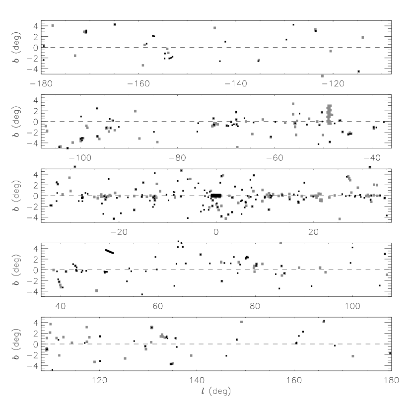
Figure 1.— The locations of archival observations used for this survey. Black squares are Chandra observations, schematically represented with boxes that have an area equal to that of the ACIS-I. Grey rectangles are XMM-Newton observations, schematically represented with boxes that have an area equal to that of one EPIC MOS.

2. Observations

We attempted to identify new magnetars by searching for sources with periodic X-ray pulsations in archival Chandra and XMM-Newton observations of the Galactic plane. We included observations with a Galactic latitude $|b|$$<$5^∘ that were public as of January 2007. For both observatories, we required that some of the data were taken in an imaging mode. For Chandra, we further rejected observations taken with the gratings in place. For XMM-Newton, we rejected all observations shorter than 10 ks, because they were often affected by background flares throughout their entire duration. In total, we searched 506 Chandra observations, and 441 XMM-Newton observations. The coverage on the sky is illustrated in Figure 1. Within a Galactic longitude of $|l|$$<$10^∘ and a latitude $|b|$$<$5^∘, which encloses about half of the mass of the Galaxy (e.g., using the model in Launhardt, Zylka, & Mezger 2002), these observations cover about 6% of the sky. Closer to the Galactic plane, within $|l|$$<$10^∘ and $|b|$$<$0.5^∘, the observations cover 25% of the sky.

The raw event lists and calibration data were downloaded from the High Energy Astrophysics Science Archive Research Center. We processed the event lists produced by each observatory in the standard manner, in order to extract events for sources that we could search for periodic variability.

2.1. Chandra Data Preparation

The Chandra data were processed using CIAO version 3.4. As we were only interested in the arrival times of events, we did not apply the latest calibration. We started with the default level 2 event files, and removed any time intervals during which flares from the particle background caused the total event rate from the detectors to increase by more than 2$\sigma$ above the mean event rate. We then generated exposure maps at a fiducial energy of 1.5 keV (i.e., the peak of the detector effective area), and binned the event lists to produce images in the 0.5–8.0 keV band. These were used to search for point sources using the routine wavdetect (Freeman et al., 2002). For computational efficiency, we searched a series of three images using sequences of wavelet scales that increased by a factor of $\sqrt{2}$: a central, un-binned image of 8.5′ by 8.5′ searched over scales of 1–4 pixels, an image binned by a factor of two to cover 17′ by 17′ searched over scales of 1–8 pixels, and an image binned by a factor of four to cover the entire field searched over scales of 1–16 pixels. The source lists from each image were combined for each observation, favoring the positions derived from the images with the highest spatial resolution for sources detected at multiple scales. We did not attempt to discriminate real sources from detector artifacts, such as the boundaries of the individual charge-coupled devices (CCDs), at this stage of the algorithm.

We then extracted events from each source, using a radius defined to enclose 90% of the point spread function (PSF) at 4.5 keV. In this case, a relatively higher energy was used so that we would not exclude photons from sources with hard spectra. The radius was dependent on the offset from the aim point in arcminutes ($\theta$), and was parameterized based on simulations with the CIAO tool mkpsf as

$$r=3.27+0.342\theta+0.020\theta^{2}+0.019\theta^{3},$$ (1)

where $r$ is the radius in pixels (0$\farcs$492). We corrected the arrival times of the events to the Solar System barycenter using the tool axbary.

2.2. XMM Data Preparation

The XMM-Newton event lists from the European Photon Imaging Camera (EPIC) were analyzed using version 7.0 of the Science Analysis Software, CIAO 3.4, and the High Energy Astrophysics Software version 6.3.0. We examined the lists from each active imaging detector separately, starting with the files from the archive. For most observations, the same field was observed with three independent cameras: one pn CCD array and two metal-oxide-silicon [MOS] CCD arrays. We removed time intervals during which particle events caused the event rate from the detector to flare more than two standard deviations above the mean rate. This selection was generally successful at removing particle flares, but in many cases the entire observation for a given camera was affected by flares, which rendered this automatic algorithm useless. We discarded data from individual cameras (usually the pn) for observations too badly affected by flares.

We then created images of the 0.2–12 keV events, binned to 4″ resolution. The standard data selection was applied to make the images, in order to remove events near the edges of the detector chips and bad pixels, and to reject events that were likely to be cosmic rays (pattern $\geq$4 for the pn and $\geq$12 for the MOS). We then generated matching exposure maps. We searched for point sources using the routine ewavelet, separately for each observation. At this stage of the algorithm, we did not attempt to discriminate real sources from detector artifacts, nor did we attempt to verify that sources detected in one camera were present in the others. We extracted event lists from individual sources using the radius produced by ewavelet, which generally was $\approx$15″ and enclosed $\approx$50% of the PSF. The arrival times of the photons were corrected to the solar system barycenter using the tool barycen.

2.3. Identifying Candidate Signals

For sources with at least 100 total events from either observatory (including background), we computed Fourier periodograms to search for periodic signals. The range of periods searched for both instruments was designed to encompass those of known magnetars with X-ray pulsations, 5–12 s (Woods & Thompson, 2006). However, we note that after our analysis was completed, Camilo et al. (2007) announced the discovery at radio wavelengths of 2 s pulsations from 1E 1547.0-5408. Periods this short would generally only be identifiable in XMM-Newton EPIC-pn data with our search.

For the Chandra data, we used the Rayleigh statistic ($Z_{1}^{2}$; Bucceri et al., 1983). We searched for signals with frequencies between 1.5 times the Nyquist frequency (i.e., $1.5\times 1/2t_{\rm bin}$, where $t_{\rm bin}$ is the interval at which the data were read out) and 10% of the inverse of the total time interval of the observation (i.e., $0.1/T_{\rm exp}$) to avoid red noise. We used a frequency step corresponding to the inverse of the total time interval ($1/T_{\rm exp}$). For most observations, the data were read out every $t_{\rm bin}$=3.1 s, so the highest frequencies searched correspond to periods of 4.1 s. Observations typically lasted between 1.2 ks and 120 ks, so we could identify signals with periods at the upper range of at least 120 s, and in some cases 12,000 s.

For the XMM-Newton data, the Rayleigh Statistic was computationally inefficient to compute for pn observations of bright sources, so we computed discrete fast Fourier transforms. The data were padded so that the number of points in the transform was a power of 2, so the frequency resolution was generally finer than $1/T_{\rm exp}$. The maximum frequency considered was the Nyquist frequency for the data. The pn data was taken with a time resolution of at least 73.4 ms, providing sensitivity to periods as short as 0.15 s. The MOS data was taken with a time resolution of at least 2.4 s, and so our search was sensitive to periods as short as 4.8 s. The lowest frequency considered was 0.1/$T_{\rm exp}$.

The confidence with which we could exclude that any given signal was produced by random noise depended upon the number of trial signals examined, $N_{\rm trial}$. The typical Chandra observation lasted 20 ks, and contained 3 sources with $>$100 counts, and had a time resolution of 3.1 s, so that there were $N_{\rm trial}$$\approx$20,000 trial frequencies in the ensemble of periodograms from each observation. The typical XMM-Newton observation also lasted 20 ks, and contained $\approx$25 sources per camera with $>$100 counts. For each MOS detector, with a time resolution of 2.4 s, the typical set of periodograms contained $N_{\rm trial}$$\approx$200,000 trial periods per observation. For the pn detector, with a time resolution of 73.4 ms, the typical set of periodograms contained $N_{\rm trial}$$\approx$$1.8\times 10^{8}$ trial periods. In total, we searched $1.7\times 10^{11}$ trial periods, the vast majority of which were from the high-time-resolution data taken with the EPIC pn.

The powers produced by random noise in a periodogram in which $n$ measurements have been averaged are distributed as a chi-squared function with $2n$ degrees of freedom. Following (Ransom et al., 2002), we refer to the measured Fourier powers with $n$=1 as $P_{\rm meas}$, and normalize them so that the mean power produced by white noise is 1. The chance probability that noise would produce a signal larger than $P_{\rm meas}$ can be determined from an exponential distribution:

$${\rm prob}=1-(1-e^{-P_{\rm meas}})^{N_{\rm trial}}\approx N_{\rm trial}e^{-P_{\rm meas}},$$ (2)

where the approximation is valid for $P_{\rm meas}$$\gg$1 (Ransom et al., 2002). Given the large number of trials for our entire search, a signal that had a $<$0.1% chance of resulting from noise must have a power $P_{\rm meas}$$>$32.8. Such a signal would be detected at a confidence level equivalent to 3$\sigma$ over the entire search, or 8$\sigma$ in a single trial.

However, a signal could also be considered significant if it was detected with a lower power in multiple observations, as one might hope would occur given that XMM-Newton has three separate cameras that observe the same patch of the sky. For instance, given two signals $P_{\rm meas,1}$ and $P_{\rm meas,2}$ at the same frequency, the chance probability that their sum exceeds some value is a chi-squared distribution with 4 degrees of freedom:

$${\rm prob}\approx N_{\rm trial}(1+P_{\rm meas,1}+P_{\rm meas,2})e^{-(P_{\rm meas,1}+P_{\rm meas,2})}$$ (3)

(see Ransom et al., 2002, for the general form for summing an arbitrary number of signals). If we take $P_{\rm meas,1}=P_{\rm meas,2}$, for example, a signal has a $<$0.1% of resulting from noise if it appeared with $P_{\rm meas,1}$$>$17 in both observations. In principle, one could devise an algorithm that searched through all of the periodograms from the same source, and sum the powers at each frequency to search for signals that repeat in the data. In practice, however, the periodograms were not all computed with the same frequency resolution, which makes such an effort difficult. Moreover, when considering observations separated in time, one also has to be concerned that some candidate signals drifted in frequency, either because of the spin-down of an isolated pulsar, or Doppler shifts for a pulsar in a binary (see, e.g., Vaughan et al., 1994, for further discussion).

Therefore, we have adopted a simplified approach in examining candidate signals, by recording all signals with powers with less than a 1% chance of resulting from noise in a search of a single source. For Chandra ACIS, the threshold power is generally $P_{\rm meas}$$>$17. For the XMM-Newton MOS, the threshold power is typically $P_{\rm meas}$$>$19, whereas for the pn the power is $P_{\rm meas}$$>$26. Any candidate signal was inspected to determine its significance.

With these search criteria, our results up to this point were dominated by signals that are non-periodic noise or detector artifacts. In both Chandra and XMM-Newton data, we detected low-frequency noise from astrophysical flares in the count rates of individual sources such as pre-main-sequence stars, and from background flares that our filtering algorithm failed to remove. From Chandra ACIS, we detected signals from sources that fell near chip boundaries, at the harmonics and beat periods of the satellite dither (700s in the $x$-direction, 1000s in the $y$). For the XMM-Newton EPIC, particularly the pn, we found signals with a range of periods that appeared to be related to hot columns and chip boundaries, particularly in observations with high particle background. We are not certain of the origin of these signals from the EPIC. The spurious signals introduced by the detector generally shared the feature that they could be found in multiple sources at the exact same frequency during an observation. Therefore, we have removed from consideration any signals that appeared in two or more sources on the same detector in the same observation. After removing such signals, we found 358 sources with candidate signals in the Chandra observations, and 1380 sources (some of which are duplicates) with signals from XMM-Newton.

These signals still turned out to be dominated by low-frequency noise and detector artifacts, which could be quickly determined by visually inspecting the power spectrum. Therefore, for the final step, we scrutinized $\approx$1700 power spectra by eye to remove the remaining examples that were clearly noisy, and to remove sources that appeared to be detector artifacts. We defined a signal as significant if it had a power $P_{\rm meas}$$>$32.8 in a single observation or had a power larger than the single-observation threshold in two or more observations. We found a few sources with significant periodic signals that we could not attribute to noise or detector artifacts. We describe the previously-known and new sources separately below.

Table 1Candidate Periodic Signals

Source	ObsID	Detector	Counts	$T_{\rm exp}$	Period	$P_{\rm meas}$
				(ks)	(s)
CXOU J174728.0–321445	4567	ACIS-S	2076	42.1	4910$\pm$20	199
	4566	ACIS-S	1489	28.3	4790$\pm$50	81.9
CXOU J182531.4–144036	5341	ACIS-I	548	18.0	780$\pm$3	36.4
					5000$\pm$100	42.8
XMMU J124429.7–630407	010948101	pn	491	49.0	475.0$\pm$0.6	21.3
		MOS-1	187	52.0	474.6$\pm$0.8	14.4
		MOS-2	162	52.0	474.5$\pm$1.0	3.5
	010948401	pn	403	39.3	475.1$\pm$0.5	23.5
		MOS-1	145	41.7	476.7$\pm$1.7	11.1
		MOS-2	141	41.1	473.9$\pm$1.2	11.8
XMMU J185330.7–012815	0201500301	pn	20637	20.0	238.2$\pm$0.1	74.2
		MOS-1	6781	20.1	238.4$\pm$0.2	39.1
		MOS-2	6953	20.2	238.4$\pm$0.2	26.3

Note. — The columns are as follows: the source names; the identifiers of the observations in which the signals were found; the detector with which the sources were observed; the total number of counts extracted for the source (includes background); the exposure times of the observations; the periods, which were computed by tracking the phases of the oscillations; and the power which the source was identified in the initial power spectrum.

2.3.1 Known Sources

Most of the signals were from previously-identified pulsars. These confirmed that our algorithm worked as intended. In our Chandra observations, we identified the high-mass X-ray binary (HMXB) 4U 1145–619 (White et al., 1978; Rutledge et al., 2005), CXOU J164710.2–455216 (Muno et al., 2006), and two sources toward the Galactic center (CXOC J174532.3–290251 and GXOGC J174532.7–290552; Muno et al., 2003). In the XMM-Newton observations, we identified the pulsars Geminga (Halpern & Holt, 1992; Jackson & Halpern, 2005) and PSR J1513–5908 (Seward & Harnden, 1982), the HMXB Sct X-1 (Koyama et al., 1991; Kaplan et al., 2007), and the magnetars 1E 1048.1–5937 (Seward, Charles, & Smale, 1986; Tiengo et al., 2005), 1RXS J170849.0–400910 (Sugizaki et al., 1997; Rea et al., 2005), SGR 1806-20 (Murakami et al., 1994; Mereghetti et al., 2005), SGR 1900+14 (Hurley et al., 1999; Mereghetti et al., 2006a), XTE J1810–197 in outburst (Ibrahim et al., 2004; Halpern & Gotthelf, 2005), and 1E 2259+586 (Fahlman & Gregory, 1981). The list above includes 7 of the 12 confirmed magnetars in the Galaxy.

It is notable, however, that several magnetars were not detected in our search, despite being the targets of archival Chandra and XMM-Newton observations. Here, we summarize the difficulties encountered identifying several examples:

1E 2259+586 was not identified with Chandra because it saturated the detector during an imaging observation.

1E 1048.1–5937 and 1RXS J170849.0–400910 were not identified with Chandra because they were only observed with the gratings in place. These cases are not a serious concern, because such bright sources are rare, and so almost never are found serendipitously in the fields of Chandra and XMM-Newton.

SGR 1806–20 and SGR 1900+14 were not identified by Chandra while in quiescence. Although their signals were present in the data, their powers were below our search threshold. All of the above sources were identified with XMM-Newton.

4U 0142+61 was not identified with either Chandra or XMM-Newton. This is partly because the source had a small pulse fraction (4% rms), but also because of the detector modes with which the source was observed. With Chandra the source either saturated the detector during imaging observations, or was observed with the gratings in place. With XMM-Newton, only the MOS2 camera was active, and the magnetar only produced a signal above the single-observation threshold ($P_{\rm meas}$$>$18) in one of the two observations. That signal ($P_{\rm meas}$=24.7) was below the threshold for our entire search, and so can not be considered a detection as part of our blind search. However, had that source been observed with the pn active, we would have identified it.

1E 1841–045 also was not identified with Chandra or XMM-Newton. With a fractional rms amplitude of 13% rms, it did not produce a significant signal in the Chandra data. The XMM-Newton observations of this source were too short ($<$10 ks) to be included in our search. A longer XMM-Newton observation would almost certainly have identified this source.

SGR 1627–41, AX J1845.0–0258, and XTE J1810–197 in quiescence were all too faint to produce detectable pulsations, even in searches targeted at their known or suspected spin periods (Gotthelf et al., 2004; Tam et al., 2006; Mereghetti et al., 2006b). These objects, and possibly the newly-identified magnetar 1E 1547.0-5408, represent a class of magnetars from which pulsations could only be detected intermittently, or perhaps not at all, in a search like ours.

2.3.2 Newly-Identified Sources

Four sources produced periodic signals that have not been previously reported. In Table 1 we have listed basic information about each source and signal. Figures 2 and 4 contain the Fourier power spectra in which the candidate signals were discovered. The power spectra provided initial estimates of the pulse periods. We then refined the periods by (1) computing pulse profiles from non-overlapping intervals between 1000 and 10,000 s long (depending upon the number of counts from the source), (2) measuring their phases by fitting a sinusoid to the data, and (3) modeling the differences between the assumed and measured phases using first-order polynomials. The pulse profiles are displayed in Figures 3 and 5. Below we remark on some peculiarities to each source:

Figure 2.— Power spectra from sources with periodic variability in archival Chandra observations. The left panels display power spectra from the two observations of CXOU J174728.0–321445, and the right panel displays it from CXOU J182531.4–144036. The downward-pointing arrows denote the fundamental and two harmonics of the $\approx$700 s and $\approx$1000 s dither periods for the satellite. The $\approx$700 s dither period, along with beat periods between that and the 5000 s signal, are evident in the data from CXOU J174728.0–321445, because the source lay at the edge of the detector.

Figure 3.— Profiles of the periodic signals detected in archival Chandra observations. Two cycles are repeated in each pane. The left panels display the profiles of the $\approx$5000 s signals from the two observations of CXOU J174728.0–321445. The right panels display the profiles of the 780 s (top panel) and 5000 s (bottom panel) signals from CXOU J182531.4–144036. The period is printed at the bottom of each panel.

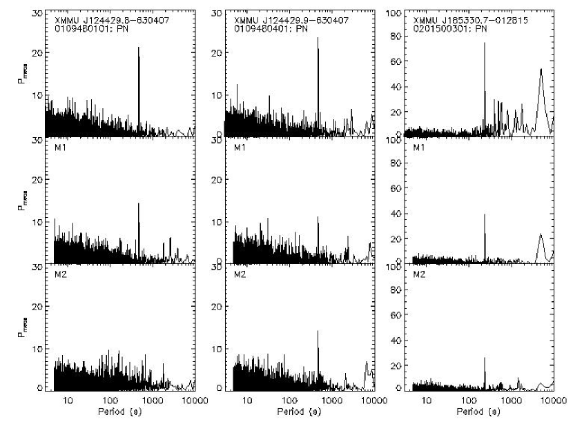
Figure 4.— Power spectra from sources with periodic variability in archival XMM-Newton observation. From left to right, we display power spectra from the first and second observations of XMMU J124429.7–630407, and from the one observation of XMMU J185330.7–012815. From top to bottom, we display data from the EPIC-pn, MOS1, and MOS2.

Figure 5.— Profiles of the periodic signals detected in archival Chandra observations. Two cycles are repeated in each panel, and data from all of the pn, MOS1, and MOS2 have been combined. From left to right, we display data from first and second observations of XMMU J124429.7–630407, and from the one observation of XMMU J185330.7–012815.

CXOU J174728.0–321445: The $\approx$5000 s period from this source is longer than 10% of the exposure time, so it would not have been identified in our search were it not for the facts that the signal has a strong harmonic near 2500 s. The source is detected in two observations. In both observations, it lies near the edge of a detector. The 707.4 s dither period is clearly detected in the data, but the $\approx$1000 s dither period (specifically, 1010.9 s in observation 4567 and 989.9 s in observation 4566) is not seen because of the orientation of the detector. In addition, signals are detected at the difference between the frequencies of the dither and the 5000 s signal. The periods from the phase connection analysis differ at the 2$\sigma$ level, so this signal may not be strictly coherent.

CXOU J182531.4–144036: This source was identified for its 780 s period. The signal is unrelated to the dither periods, which in this observation were at 999.7 s and 707.6 s. Oddly, a $\approx$5000 s period is also present in this source. We have confirmed that this 5000 s period does not appear in most sources observed with Chandra, and the profile of the 5000 s signal is more sinusoidal in this source than in CXOU J174728.0–321445. However, only 4 cycles of the 5000 s signal were covered by the observation, so this signal may be low-frequency non-periodic noise that randomly produced a strong peak in the power spectrum.

XMMU J124429.7–630407: A 475 s period was detected from this source in 5 of 6 trial power spectra from two different observations. The source is faint, and the non-detection with the MOS2 in observation 010948101 can be ascribed to unfavorable noise.

XMMU J185330.7–012815: This source, also known as AX J1853.3-0128, exhibited a 238 s period in all three detectors in the one observation of it. The analysis of the phases of this source indicate the signal is not coherent, as the phases vary by $\approx$0.1 cycles with a time scale of $\approx$5000 s. The periodic signal from this source was identified independently by J. Halpern and E. Gotthelf, who also carried out spectroscopy of its optical counterpart, and suggest that it is a cataclysmic variable (private communication).

We note that it is curious that the period of the signal from XMMU J124429.7–630407 is within 2$\sigma$ of being a factor of 2 longer than the period of the signal from XMMU J185330.7–012815. We have not been able to identify any systematic effect that might explain both signals. In our search, we did not find similar significant signals from any of the thousands of other sources that we examined. The signals are unlikely to be detector artifacts, because they are detected in the pn and both MOS cameras. Having failed to identify any causes intrinsic to the spacecraft, on-board computers, or data processing, we believe that they are astrophysical, and that the factor of two difference between them is simply a coincidence.

3. Discussion

The periodic signals that we have detected from previously-unidentified sources all have periods longer than 100 s. Although there is a chance that some of these systems are neutron stars, we expect that most of them belong to the much-larger population of magnetically-accreting white dwarfs, either polars or intermediate polars (e.g., Norton & Watson, 1989; Schwarz et al., 2002; Ramsay & Cropper, 2003; Muno et al., 2003). Accreting white dwarfs typically have luminosities of $10^{30}-10^{32}$ erg s^-1, so that given their count rates, they could be located as close as 50 pc (for XMMU J185330.7–012815) or as far as 5 kpc (for XMMU J124429.7–630407). As members of the local Galactic neighborhood they will be distributed over the entire sky, not just within $|b|$$<$5^∘, our targeted survey of the Galactic plane is not particularly efficient at finding cataclysmic variables. Therefore, we do not discuss them further.

In the context of a search for magnetars, it is notable that no new source was found to exhibit periodic variability with periods in the range of known magnetars that are pulsed in X-rays, 5–12 s. To understand the lack of detections of obvious candidate neutron stars, we need to compute the fraction of the Galaxy that was covered by our survey. If the properties of magnetars as a population were bettern known, we would do so by assuming distributions for their luminosities and pulse amplitudes, and carry out a maximum-likelihood or Monte-Carlo calculation to model the observed population (e.g., Faucher-Giguère & Kaspi, 2006; Lorimer et al., 2006). However, the intrinsic distributions for the luminosities and pulse fractions of magnetars are poorly constrainted. Some guidance can be obtained from models that explain the pulsations as originating from single bright spots on their surfaces. Özel (2002) find that the fractional amplitudes of pulsations are largest when the hot spot is located on the equator, and viewed from the equator. However, the amplitude drops by $\approx$50% when the spot and viewer have a latitude $>$50^∘. Therefore, we roughly estimate that any given magnetar will be easily detectable over $\approx$65% of the sky.

Unfortuntely, as we describe below, the luminosities of magnetars are highly variable, and cannot be predicted by first principles because the mechanism causing the variability is not understood (e.g., Woods et al., 2004; Muno et al., 2007). Therefore, in the following we only present some representative cases. The total Galactic populations for our fiducial examples are then calculated in two steps, first computing the depth along the line-of-sight through the Galaxy to which our observations were sensitive, and second estimating the fraction of the stellar mass in the Galactic spiral arms that was enclosed by our observations.

3.1. Depth of the Survey

We compute the depth ($D$) through the Galaxy that each observation was sensitive for any given luminosity ($L_{\rm X}$) and limiting total number of counts ($C_{\rm lim}$) from:

$$C_{\rm lim}/T_{\rm exp}=\xi_{\rm det}(N_{\rm H}[l,b,D])\frac{L_{\rm X}}{4\pi D^{2}},$$ (4)

where $\xi_{\rm det}(N_{\rm H}[l,b,D])$ is the conversion factor between flux and count rate for each detector. This factor depends additionally upon the Galactic absorption $N_{\rm H}$, which in turn is a function of the distance $D$ to a source and its position in the Galactic plane, $l,b$. We computed $f(N_{\rm H})$ for both the Chandra ACIS-I and for the XMM-Newton EPIC pn behind the medium filter using the Portable, Interactive Multi-Mission Simulator, assuming several trial spectra and a range of $N_{\rm H}$. We have neglected some other factors that do not significantly affect our results, the choice of filters for XMM-Newton (an $\approx$5% effect on $\xi$), and hydrocarbon build-up on the ACIS (negligible for sources with $N_{\rm H}$$\gtrsim$$10^{22}$ cm^-2).

Vignetting as a function of offset from the aim point is a small effect for Chandra, reducing the count rate from a source by $\approx$20% at an offset of 8′. We have neglected vignetting in our Chandra observations. However, it is a large effect for XMM-Newton, reducing the count rate by 50% at an offset of 10′. Therefore, we have accounted for vignetting in our XMM-Newton observations by reducing the flux-to-counts conversion $\xi$ by 33% from the on-axis value obtained from PIMMS, which is the mean reduction over the inner 10′. We estimate that our simple treatment of the vignetting introduces an uncertainty of $<$15% on the depth of the survey.

The spectra of magnetars are generally described as the sum of a blackbody component with a temperature of $kT$$\approx$0.6 keV and a soft power-law tail with photon index $\Gamma$$\approx$3 (e.g., Woods & Thompson, 2006). The overall spectrum can be roughly approximated as a $\Gamma$=2 power law, so we take that as our fiducial spectrum. Choosing instead a softer $\Gamma$=3 power law results in values of $D$ that are up to 30% smaller (depending upon the absorption through the line of sight; see below), while choosing a harder $kT$=0.6 keV blackbody increases $D$ by up to 20%.

We estimated the absorption as a function of distance along different lines of sight using models for Galactic optical and infrared extinction. For most of the Galactic plane, we linearly interpolated visual extinction values ($A_{V}$) from the model of Drimmel et al. (2003), and converted them to $K$ band extinction values using the relation $A_{K}/A_{V}=0.11$ (Rieke & Lebofsky, 1985; Mathis, 1990). However, within the central 25^∘ of the Galaxy the model extinction from Drimmel et al. (2003) was significantly lower than that observed (e.g., Launhardt et al., 2002), so instead we interpolated values of the $K_{s}$ band extinction from the table in Marshall et al. (2006). We then converted the $K$ band extinction (ignoring the 5% difference in $A_{K}$ and $A_{K_{s}}$) into a column density using $N_{\rm H}=1.6\times 10^{23}A_{K}$ cm² (Rieke & Lebofsky, 1985; Predehl & Schmitt, 1995). Absorption through the Galactic plane can reduce the flux observed from a source by up to a factor of 30 compared to the value without absorption. We tested different values for $N_{\rm H}/A_{K}$ in the range $(1.2-2.1)\times 10^{22}$ cm² (representing values from, e.g., Glass, 1999; Tan & Draine, 2004), and found that the uncertainty in $D$ introduced by our choice of absorption model is $\approx$15%.

The depth of our survey depends strongly upon the assumed luminosity and the fractional root-mean-squared (rms) amplitude of the pulsations ($A_{\rm rms}$) for which we are searching. The rms amplitude enters consideration because it determines $C_{\rm lim}$:

$$A_{\rm rms}=1.13\left(\frac{2P_{\rm sig}}{C_{\rm lim}}\right)^{1/2}{\rm sinc}^{-1}\left(\frac{\pi}{2}\frac{\nu}{\nu_{\rm Nyq}}\right),$$ (5)

where $P_{\rm sig}$ is the intrinsic power of a detectable signal, the factor of 1.13 is an average correction that accounts for the fact that signals will often fall between independent Fourier bins, and the ${\rm sinc}$ term takes into account the attenuation of the power of a signal as its frequency $\nu$ approaches the Nyquist value $\nu_{\rm Nyq}$ (Vaughan et al., 1994). The intrinsic power $P_{\rm sig}$ detectable in a search must be determined using the distribution of noise powers, as described in Vaughan et al. (1994). For a search threshold of $P_{\rm meas}$=32.8, the expected value (50% confidence) is $P_{\rm sig}$=31.8, and the power detectable in 90% of trials is $P_{\rm sig}$=48.0. In the following we will use the 90% confidence level, $P_{\rm sig}$=48.0. The value of $D$ computed for $P_{\rm sig}$=31.8 is $\approx$10–20% larger than the value for $P_{\rm sig}$=48.0.

For our depth calculation, we use two extremes as examples. The first is an easily-detectable magnetar. As our model for this, we use a faint pulsar with a high pulse fraction, such as CXOU J164710.2–455216 in Westerlund 1 (Muno et al., 2006), which had a luminosity of $L_{\rm X}$=$3\times 10^{33}$ erg s^-1 (0.5–10 keV) and a fully-modulated sinusoidal pulse profile with $A_{\rm rms}$=0.71. Pulsations like this could be detected in 90% of trials with as few as $\approx$120 photons. The depth probed by any given observation scales as $L_{\rm X}^{1/2}$ and linearly with $A_{\rm rms}$, so the easily-detectable example is equivalent to a bright magnetar like SGR 1900+14, with $L_{\rm X}$=$10^{35}$ erg s^-1 (0.5–10 keV) and a sinusoidal pulse profile with $A_{\rm rms}$=0.12 (Hurley et al., 1999). In the top panel of Figure 6, we plot the depth at which each observation would have been sensitive as a function of exposure time for our easily-detectable example. Only 10% of the Chandra observations and 20% of the XMM-Newton observations probe the entire depth of the Galactic plane to a distance of 24 kpc from Earth.

The other extreme is a barely-detectable pulsar, with a low luminosity $L_{\rm X}$=$3\times 10^{33}$ erg s^-1 and a small pulse fraction $A_{\rm rms}$=0.15. This example is chosen to have been just detectable in observations comparable to those of XTE J1810–197 in quiescence, for which $L_{\rm X}$=$2\times 10^{33}$ erg s^-1 (0.5–10 keV), and from which pulsations were not detected to a limit of $A_{\rm rms}$$<$17% (Gotthelf et al., 2004). A source with $A_{\rm rms}$=0.15 would require 2800 photons to be identified in 90% of trials. Consequently, a search sensitive to our barely-detectable pulsar would cover a factor of $\approx$5 less depth than a search for easily-detectable magnetars like the one in Westerlund 1. We display the depth of a survey for a barely-detectable magnetar in the bottom panel of Figure 6. None of the archival observations would probe the entire Galaxy when searching for our barely-detectable pulsar.

Figure 6.— The depth through the Galaxy that each observation sampled, plotted as a function of its exposure time. Triangles illustrate Chandra ACIS observations, and circles XMM-Newton EPIC-pn observations. The EPIC-pn has a larger effective area than ACIS, so the XMM-Newton observations are systematically deeper for a given exposure. Filled symbols indicate the depth at which we are sensitive to an easily-detectable pulsar with $L_{\rm X}=3\times 10^{33}$ erg s^-1 and $A_{\rm rms}$=70%. Open symbols indicate the depth at which we are sensitive to a barely-detectable pulsar with $L_{\rm X}=3\times 10^{33}$ erg s^-1 and $A_{\rm rms}$=15%. The dashed line at a depth of 24 kpc demarks observations that proble the entire Galaxy; larger depths are no longer meaningful because they extend beyond the distribution of young stars.

3.2. Fraction of Young Stars Enclosed by the Survey

In order to estimate the number of magnetars in the Galaxy and their birth rates, we need to know the fraction of the Galaxy that we have meaningfully surveyed for magnetars. Magnetars have massive progenitors: neutron stars form from stars within inital masses $>$8$M_{\odot}$ (Heger et al., 2003), and there is evidence that magnetars form from $>$30 $M_{\odot}$ stars (Gaensler et al., 2005; Figer et al., 2005; Muno et al., 2006). The lifetimes of magnetars are thought to be $\sim$$10^{4}$ yr (Kouveliotou et al., 1999; Gaensler et al., 1999), so even if some magnetars receive kicks of $\sim$1000 km s^-1, they will be found within $\sim$10 pc of their birth place. Most massive stars are concentrated in the Galaxy’s spiral arms, so we have calculated the fraction of the stellar mass in the spiral arms that our observations have covered.

We use the model for the stellar mass in the spiral arms from Wainscoat et al. (1992).The locations of the arms are defined as a logarithmic spiral:

$$\theta(R)=\alpha\log(R/R_{\rm min})+\theta_{\rm min},$$ (6)

where $R$ is the radial distance from the Galactic center, $\theta$ is the azimuthal angle in radians (with $\theta$=0 along the line connecting the Earth to the Galactic center, and 0$\leq$$\theta$$<$$\pi$ for $\sin l$$\leq$0), $R_{\min}$ is the radial distance at which the arms start, $\theta_{\rm min}$ is the angle at which the arms start, and $\alpha$ is the winding constant. We define four main spiral arms, and one smaller, “local arm.” Each arm is assumed to extend through an angle $\theta_{\rm ext}$, out to a maximum radial distance of $R_{\rm max}$=15 kpc. The values of $\alpha$, $R_{\rm min}$, $\theta_{\rm min}$, and $\theta_{\rm ext}$ are listed in Table 2, taken directly from Wainscoat et al. (1992). The parameters assume the Earth is 8.5 kpc from the Galactic center.

Table 2Spiral Arm Parameters

Arm	$\alpha$	$R_{\rm min}$	$\theta_{\rm min}$	$\theta_{\rm ext}$
	(radians)	(kpc)	(radians)	(radians)
1	4.25	3.48	0.000	6.00
1′	4.25	3.48	3.141	6.00
2	4.89	4.90	2.525	5.47
2′	4.89	4.90	5.666	5.47
L	4.57	8.10	5.847	0.55

The stellar density along the spiral arms is given by an exponential distribution with radius $R$ and height above the plane $z$ (Wainscoat et al., 1992):

$$\rho=\rho_{0}\exp\left(-R/h-|z|/h_{z}\right),$$ (7)

where $h$=3.5 kpc is the radial scale length, $h_{z}$=90 pc is the scale height of the youngest stars in the Galactic plane, and $\rho_{0}$ is a normalization for which the exact value is unimportant, because we will divide by the total mass to obtain the fraction of the arms encompassed by the survey. The density of the spiral arms is assumed to be constant for any given $R$ within $\pm$375 pc of the center of the arm, and zero outside that radial extent. This model for the spiral arms is illustrated schematically in Figure 7. In that figure, we also plot the depth through the Galaxy for which we would detect easily- and barely-detectable pulsars in 90% of trials ($P_{\rm sig}$=48.0) for each of our archival observations. The 50% completeness level would incorporate about 20% more of the Galaxy, but using it would add the complication that a larger fraction of magnetars with $L_{\rm X}$ and $A_{\rm rms}$ above our stated limits would be missed.

For each observation, we integrated the mass enclosed along the line of sight out to the depths defined in §3.1. We assumed a field of view of 17′$\times$17′ for Chandra, which corresponds to the full ACIS-I array. We assumed a field-of-view of 20′$\times$20′ for XMM-Newton, which corresponds to the region where vignetting still provides $>$50% of the on-axis count rate for a source. The fractional mass of the spiral arms enclosed by each observation is plotted as a function of Galactic longitude in Figure 8, for the cases of easily- and barely-detectable pulsars.

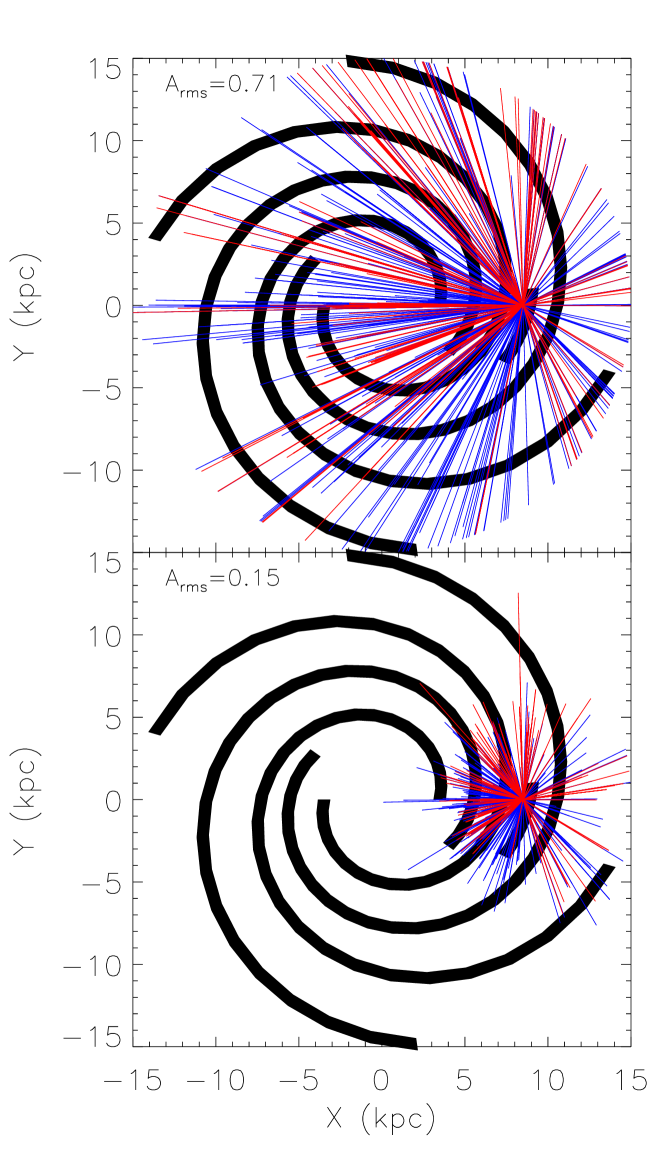
Figure 7.— The model for the Galactic spiral arms, viewed from above the north Galactic Pole, overlaid by the depth of the observations in the survey. The black lines are the model from Wainscoat et al. (1992). The blue lines represent Chandra observations, and the red XMM-Newton observations. The top panel illustrate the depth to which we are sensitive to easily-detectable pulsars, and the bottom to barely-detectable ones.

To compute the total fractional mass enclosed by the survey, we identified duplicate observations as those within 12′ of each other, and kept only the deepest of the duplicates. Then, we summed the fractional masses of the unique observations in Figure 8. We estimated uncertainties on the total fractional masses by comparing the results of the calculations made with different values for the fiducial spectrum and for the conversion between infrared extinction and X-ray absorption (§3.1). We find that our survey is 90% complete ($P_{\rm sig}$=48.0) for easily-detectable pulsars ($L_{\rm X}$=$3\times 10^{33}$ erg s^-1, $A_{\rm rms}$=71%) for 5% of the Galactic spiral arms under our standard model. The XMM-Newton and Chandra observations are about equally efficient, with Chandra surveying 2% of the spiral arms, and XMM-Newton 3% of the spiral arms. Using reasonable alternative spectra and absorption values described in §3.2, the total mass fraction surveyed can range between 3% and 7%. For barely-detectable pulsars ($L_{\rm X}$=$3\times 10^{33}$ erg s^-1, $A_{\rm rms}$=15%) our survey is complete for 0.4% of the spiral arms, with a range of 0.2–0.6% if we choose different input values. XMM-Newton and Chandra each surveyed 0.2% of the spiral arms on their own.

We note that this model for the spiral arms does not include any young stars in the central 150 pc of the Galaxy, which has been surveyed by Wang et al. (2002) and Muno et al. (in prep). For the easily-detectable magnetar case, our archival survey of this region reaches the Galactic center (Figure 7). This region contains $\sim$1% of the Galactic mass (Launhardt et al., 2002), but the star formation rate is still under debate. Figer et al. (2004) modeled the stellar population observed in the infrared there, and concluded that the star formation rate is $\sim$1% of the Galactic value. However, it is possible that star formation is skewed toward massive stars (Morris, 1993). This is suggested by indirect measurements of the Ly$\alpha$ flux in the region, which could be 10% of the total Galactic value (Cox & Laureijs, 1989; Figer et al., 1999). Depending upon the true star formation rate, the central 2^∘$\times$1^∘of the Galaxy could contribute more than half of the massive stars studied in this project.

Figure 8.— The fraction of the mass of the spiral arms surveyed by each observation, plotted as a function of Galactic longitude. Triangles illustrate Chandra ACIS observations, and circles XMM-Newton EPIC-pn observations. The EPIC-pn has a larger effective area than ACIS, so the XMM-Newton observations are systematically deeper for a given exposure. The top panel, with filled symbols, indicates the mass surveyed for which we are sensitive to an easily-detectable pulsar, with $L_{\rm X}=3\times 10^{33}$ erg s^-1 and $A_{\rm rms}$=70%. The bottom panel, with open symbols, indicates the mass surveyed for which we are sensitive to a barely-detectable pulsar with $L_{\rm X}=3\times 10^{33}$ erg s^-1 and $A_{\rm rms}$=15%.

3.3. Constraints on the Population of Magnetars

The main uncertainty in the birth rate of magnetars in the Galaxy is what the “typical” magnetar looks like. Most known examples are easily-identifiable in Chandra and XMM-Newton observations, by which we mean that they are either: (1) luminous ($L_{\rm X}$$\sim$$10^{35}$ erg s^-1) with a modest pulse fraction ($A_{\rm rms}$$\gtrsim$$13$%) or (2) faint ($L_{\rm X}$$\approx$$3\times 10^{33}$ erg s^-1) with a large pulse fraction ($A_{\rm rms}$$\approx$$70$%). Indeed 7 of 12 Galactic examples were identified blindly in our search (§2.4). However, pulsations are only intermittently-detectable from three transient magnetars — SGR 1627–41 (Mereghetti et al., 2006b), AX J1845.0–0258 (Tam et al., 2006), and XTE J1810–197 (Gotthelf et al., 2004). A fourth, 1E 1547.0–5408, has recently been identified as a magnetar through its radio emission (Camilo et al., 2007), but X-ray pulsations have not yet been confirmed (Gelfand & Gaensler, 2007). The limits on their luminosities and pulse fraction serve as guides for our barely-detectable pulsars. Therefore, there could be a significant number of magnetars that can only be identified in a blind search intermittently, when they produce outbursts.

For the purposes of this discussion, we will divide magnetars into three types: (1) the standard AXP-like sources, which are persistently bright and can be detected with pointed observations at any time, (2) the SGR-like magnetars, which can be identified by wide-field gamma-ray burst monitors from anywhere in the galaxy whenever they produce outbursts consisting of multiple soft gamma-ray bursts or occasional giant gamma-ray flares, and (3) the transient AXPs, which can only be identified by pointed observations when they produce outbursts reaching a luminosity of $\gtrsim$$10^{35}$ erg s^-1 (0.5–10 keV). This is not to suggest that these groups are mutually exclusive. For instance, the standard AXP 1E 2259+586 exhibits both short time scale bursts that appear similar to (although much fainter than) SGR bursts, and variability in its mean intensity that could be interpreted as a transient outburst with with time scales of months (Woods et al., 2004). Moreover, in addition to its soft gamma-ray bursts, SGR 1627–41 also exhibits large (factor of 20) variations in its persistent X-ray luminosity between bursts (Woods et al., 1999; Hurley et al., 2000; Mereghetti et al., 2006a), which could be interpreted as an outburst like those seen from transient AXPs (Woods et al., 2001; Kouveliotou et al., 2003; Woods et al., 2006). Instead, we use these classifications to highlight the relative ease or difficulty with which different magnetars could be detected, and thereby to answer the question, If there are many more magnetars in the Galaxy, what must they look like?

In the subsections below, we use the results of surveys most sensitive to each class of object. For standard AXPs, we use our own survey of Chandra and XMM-Newton data. For SGRs, the best constraints are provided by all-sky gamma-ray burst monitors. For transient AXPs, similar results are found using our own archival survey, and past surveys with RXTE and ASCA.

3.3.1 The Number of Standard AXPs

The standard AXPs are the easiest population to constrain, because they are easily-detectable throughout the Galaxy. Our survey of archival Chandra and XMM-Newton observations is 90% complete for finding standard AXPs for $\approx$5% of the young stellar population in the Galaxy.

Before estimating a total number of standard AXPs, however, we need to establish how many known examples lie within our random survey of the Galaxy. Only one source was identified in an observation in which it was not the target: CXOU J164710.2–455216 in Westerlund 1 (Muno et al., 2006). The other sources detected in our survey were observed as the targets of Chandra and XMM-Newton observations because they were previously known, and some thought must be taken before they can be considered as part of a random sample. Three of the standard AXPS originally were identified serendipitously during observations of other sources: 1E 1048.1–5937 during Einstein observations of the Carina nebula (Seward, Charles, & Smale, 1986), 1E 2259+586 during Einstein observations of a supernova remnant (Fahlman & Gregory, 1981), and 1E 1841–045 during ASCA observations of a supernova remnant (Vashisht & Gotthelf, 1997). In the first case, the separation on the sky between the magnetar and the central position of the original target were $\gtrsim$0.5^∘, which makes it unlikely that the magnetar would have serendipitously fallen in the field of view of a Chandra or XMM-Newton observation. In the latter two cases, the magnetars are close enough to the supernova remnants that one could have discovered them with Chandra or XMM-Newton observations, if one makes the reasonable assumption that the supernova remnant would be a sufficiently compelling target to have been observed. Therefore, we claim that 3 known magnetars lie in the random sample of the Galaxy that we surveyed.

Knowing that there are 3 easily-detectable magnetars that can be found in our search of 5% of the young stars in the Galaxy, we can determine the most likely total number of such objects in the Galaxy using the binomial distribution. The probability that $n$ pulsars out of a total population $N$ would lie in a fraction $f$ of the Galaxy is:

$${\rm prob}(n|f,N)=f^{n}(1-f)^{(N-n)}{{N!}\over{n!(N-n)!}}.$$ (8)

This can be inverted using Bayes’ theorem to give the total number of magnetars $N$, given that $n$=3 magnetars are found with the fraction $f$=0.05 of the Galaxy:

$${\rm prob}(N|f,n)=\frac{{\rm prob}(n|f,N)}{\sum_{N=n}^{\infty}{\rm prob}(n|f,N)},$$ (9)

The most likely value and 90% confidence interval for the total number of easily-detectable magnetars is $59^{+92}_{-32}$. Given that the number of known Galactic magnetars is 12, there could be $47^{+92}_{-32}$ waiting to be discovered.

The Galactic rate of core-collapse supernovae is $\sim$0.01–0.04 yr^-1 (Cappallaro et al., 1993; van den Bergh & McClure, 1994), and the radio pulsar birth rate has been recently estimated to be between $\approx$0.014 yr^-1 (Lorimer et al., 2006) and $\approx$0.03 yr^-1 (Faucher-Giguère & Kaspi, 2006). If magnetars have typical lifetimes of $\sim$$10^{4}$ yr (Kouveliotou et al., 1999; Gaensler et al., 1999), then with somewhere between 27 and 160 in the Galaxy, the magnetar birth rate would be between 0.003 and 0.016 yr^-1. The lower bound is considerably smaller than the pulsar birth rate, as would be expected if magnetars descend from $>$30$M_{\odot}$ stars (e.g., Gaensler et al., 2005). However, at the upper range, magnetars that resemble the standard AXPs could have a birth rate nearly equal to that of radio pulsars.

Figure 9.— The number of SGRs that could be present in the Galaxy, as a function of the rate at which year-long outbursts (consisting of multiple, $\lesssim$1 s soft gamma-ray bursts) recur. The solid lines shows the most likely number, given that 3 Galactic SGRs have been identified in the last 25 years, and the dashed lines show the 90% confidence limit on that number.

3.3.2 The Number of SGRs

An SGR can be identified if it produces multiple bright soft gamma-ray bursts ($\gtrsim$$10^{40}$ erg s^-1, e.g., Aptekar et al., 2001). Over the course of $\approx$25 years of monitoring, 3 Galactic SGRs have been confirmed (and one in the LMC Woods & Thompson, 2006). Their bursts typically last $\sim$0.1 s (Göğüş et al., 2001), so they are bright enough to be detected from anywhere in the Galaxy. Therefore, to estimate their total number, we only need to determine the rate at which SGRs produce detectable bursts.

For any monitoring period of length $T$, if we define an “outburst” as containing multiple individual soft gamma-ray bursts, an SGR will be identified if it produces one or more outbursts. According to Poisson statistics, if the outburst rate $r$ (where we take $r$ to have units such that the expected number of outbursts in a time $T$ is $rT$), the chance that any given source is detected will be

$${\rm prob}_{\rm det}=1-e^{-rT}.$$ (10)

Given an ensemble of $n$ sources, the probability that $m$ sources will be detected (and $n-m$ not detected) is

$${\rm prob}(m|n,rT)=(1-e^{-rT})^{m}(e^{-rT})^{(n-m)}{{n!}\over{m!(n-m)!}}.$$ (11)

This is simply a binomial distribution, which can be inverted using Bayes’ theorem to obtain ${\rm prob}(n|m,rT)$ in the same way as Equation 9.

We can receive some guidance about the rate at which SGRs are active by noting that, out of 25 years of monitoring, SGR 1806–20 has been active for $\approx$7 years, SGR 1900+14 for $\approx$4 years, SGR 0526–66 (in the LMC) for $\approx$2 years, and SGR 1627–41 for $\approx$2 months (Aptekar et al., 2001; Woods & Thompson, 2006). The bursts tend to be associated with periods of activity lasting months to years. It is clear that the activity level is variable from source to source, so we consider a range of rates.

Given $m$=3 and $T$=25 years, in Figure 9 we plot for a range of $r$ the most-likely value and 90% confidence limit for $n$. If on average one outburst is expected every 10 years, which is near the mean of the sample that has already been identified, then with 90% confidence we should have already detected all of the Galactic SGRs. However, if an SGR only becomes active once per 100 years, there could be $13^{+18}_{-7}$ in total in the Galaxy. Our best estimate is therefore that the number of Galactic SGRs is much smaller than that of standard AXPs, unless SGRs are active less frequently than once per several hundred years.

Figure 10.— The number of transient AXPs that could be present in the Galaxy, as a function of the rate at which year-long outbursts (in which the X-ray luminosity is at least $10^{35}$ erg s^-1) recur. The number of Galactic examples is calculated based on observations with ASCA, RXTE, Chandra, and XMM-Newton, which surveyed $\approx$2% of the Galaxy each year for 11 years, and discovered two transient AXPs. The solid lines shows the most likely number, and the dashed lines show the 90% confidence limit.

3.3.3 The Number of Transient AXPs

Transient AXPs would be the most difficult to identify, and could comprise the majority of the magnetars. We define an AXP as transient if it has a luminosity of $\lesssim$$10^{33}$ erg s^-1 (0.5–10 keV) for most of its current life, but increases in luminosity to $\sim$$10^{35}$ erg s^-1 for durations of on order a year (e.g., Gotthelf et al., 2004; Tam et al., 2006). We define the “outburst” as the year-long period when the AXP is luminous. Three transient AXPs are known (XTE J1810–197, CXOU J164710.2–455216, and 1E 1547.0–5408), along with one candidate (AX J1845.0–0258).

Our archival Chandra and XMM-Newton survey provides the most sensitive search for transient AXPs in quiescence. Nonetheless, when looking for a pulsar with $L_{\rm X}$=$3\times 10^{33}$ erg s^-1 (0.5–10 keV) and $A_{\rm rms}$=15%, our survey is only 90% complete for $\approx$0.4% of the Galactic young stellar population. The simple calculation (Eq. 9) assuming no new barely-detectable magnetars in $f$=0.005 of the Galaxy, implies that with 90% confidence there could be up to 540 waiting to be discovered. Unfortunately, this estimate is not a strict upper bound, because quiescent AXPs could be less luminous or have lower pulsed fractions than we have assumed.

An AXP in outburst could be detected over a larger fraction of the Galaxy, but it still requires an observation with a pointed X-ray observatory. To constrain their numbers based on AXPs in outburst, we must account for both the fraction of the young stars in the Galaxy that can be surveyed by a given observatory (Eq. 8), and the chance that AXPs in the region will produce an outburst (Eq 11). We assume that there is a population of $N$ magnetars in the Galaxy with an outburst rate $r$, and that we searched for them with a survey of duration $T$ that covered a fraction $f$ of the magnetar birth places. Then, the probability that $m$ magnetars will be found is the joint probability that $n$ out of $N$ magnetars will lie in the survey region, and that $m$ out of $n$ will produce outbursts:

$${\rm prob}(m|rT,f,N) =$$

$$\sum_{n=m}^{N} (1-e^{-rT})^{m}(e^{-rT})^{(n-m)}\frac{n!}{m!(n-m)!}$$ (12)

$$\times f^{n}(1-f)^{(N-n)}\frac{N!}{n!(N-n)!}.$$

This can be inverted using Bayes’ theorem, in order to derive the probability that there are $N$ magnetars given that $m$ are found with outbursts at a rate $r$ in a fraction $f$ of the Galaxy, ${\rm prob}(N|m,rT,f)$, as in Equation 9. Here, because we are dealing with transient sources, $f$ represents the fraction of the young Galactic population searched per year, which is the duration of a typical outburst.

We can estimate the rate of outbursts from transient AXPs from the four known examples (here we assume that the candidate is a genuine example). AX J1845.0–0258 and XTE J1810–197 have each exhibited only one outburst each, in 1993 and 2002 respectively, which in both cases led to their discoveries (Torii et al., 1998; Ibrahim et al., 2004; Gotthelf et al., 2004; Tam et al., 2006). In contrast, CXOU J164710.2–455216 entered into outburst only a year after its discovery (Muno et al., 2006, 2007; Israel et al., 2007), and 1E 1547.0–5408 has brightened to $\sim$$10^{35}$ erg s^-1 (0.5–10 keV) on at least two occasions in the last 10 years (Gelfand & Gaensler, 2007; Camilo et al., 2007). Taken together, these results suggest that the mean recurrence time is about once every 8 years. As we did for SGRs, we consider below a range of rates around this value.

To compute the fraction of the young Galactic population that has been searched for transient AXPs, we need to take into account how the known examples were discovered. Two transient AXPs were discovered serendipitously: XTE J1810–197 in an RXTE observation of SGR 1806-20 (Ibrahim et al., 2004), and AX J1845.0–0250 in an ASCA observation of Kes 75 (Torii et al., 1998). We consider these to be useful examples for estimating the total Galactic population. The other two probably would not have been idenitified as transient AXPs were it not for unusual circumstances. The outburst from CXOU J164710.2–455216 was identified because it produced a hard X-ray burst that was detected by Swift, but that burst probably would have been ignored if the source had not been previously identified in quiescence (Israel et al., 2007). We have taken into account objects like CXOU J164710.2–455216 to the Galactic population in §3.3.1, so we do not include it here. 1E 1547.0–5408 was positively dentified as a magnetar through radio observations of a variable, point-like X-ray source in a supernova remnant that was studied deliberately (Gelfand & Gaensler, 2007; Camilo et al., 2007). X-ray pulsations have not yet been confirmed from this source, so we do not consider it here.

Based on the above considerations, we now calculate the fraction of young stars that RXTE, ASCA, Chandra, and XMM-Newton surveyed per year during their lifetimes, in the same manner as in §3.1–3.2. We assume that the target magnetar would have $L_{\rm X}$=$10^{35}$ erg s^-1 (0.5–10 keV), and a net number of counts determined by the observations in which XTE J1810–197 and AX J1845.0–0258 were identified. For RXTE  XTE J1810–197 was detected with $\approx$6 counts s^-1 in a 2.6 ks observation with the Proportional Counter Array (PCA; Ibrahim et al., 2004), so we assume that a pulsar would require $1.6\times 10^{4}$ total counts to be identifiable. We take the PCA field-of-view to be 50′$\times$50′, and use a count-to-flux conversion that is 33% of the on-axis value. We find that the RXTE PCA has surveyed $\approx$2% of the Galaxy down to this sensitivity during the last 11 years, and $\approx$0.7% in any given year. For ASCA  AX J1845.0–0258 was detected with $\approx$1000 net counts in each Gas Imaging Spectrometer (Torii et al., 1998). Vignetting drastically reduces the count rates from sources off-axis, so we assume a field-of-view of only 20′$\times$20′, and use a flux-to-count conversion that is 33% smaller than the on-axis value. We find that ASCA observations were sensitive to bright magnetars over $\approx$3% of the Galaxy during its 7 year lifetime, and $\approx$1% of the Galaxy per year. Finally, we find that Chandra surveyed $\approx$0.5% of the Galaxy per year over the last 7 years, and that XMM-Newton surveyed $\approx$1% of the Galaxy per year over the last 6 years. Taken together, and accounting for overlaps, we find that over the last 11 years (since the launch of RXTE), $\approx$2% of the Galaxy has been surveyed by a pointed X-ray observatory each year.

In Figure 10, we plot the constraints on the total number of transient AXPs, given that two were identified during observations of $f$=0.02 of the young Galactic population each year for $T$=11 yr. Transient AXPs are probably the largest undiscovered population of magnetars. For instance, if the average transient AXP produces outbursts at a rate of one per 10 years, then there could be $190^{+390}_{-110}$ of them in the Galaxy. The upper bound is comparable to the number of quiescent magnetars that we estimate could be present based on archival Chandra and XMM-Newton observations. For a lifetime of $10^{4}$ yr (Kouveliotou et al., 1999; Gaensler et al., 1999), this implies a brigh rate of 0.008–0.06 yr^-1. The lower bound is $\approx$50% of the radio pulsar birth rate, whereas the upper bound exeeds the higher estimate of the pulsar birth rate from Faucher-Giguère & Kaspi (2006). The higher rate would be large compared to the estimated Galactic supernova rate. However, it is possible that transient magnetars have significantly longer lifetimes than have been estimated based on the energy budgets of the persistent examples (e.g., Kouveliotou et al., 1999; Gaensler et al., 1999), in which case the birth rates would be correspondingly lower.

4. Conclusions

We have serached archival Chandra and XMM-Newton observations for X-ray pulsars, in order to constrain the Galactic population of magnetars. Although we found four objects with periodic variability on time scales of 200–5000 s (Figs. 2–5 and Table 1), we found no sources that were obviously magnetars. The archival observations that we used covered a moderate fraction of the young stellar populations from which magnetars descend. Our search was sensitive to the standard, easily-detectable AXP-like magnetar ($L_{\rm X}$=$10^{35}$ erg s^-1 [0.5–10 keV] and a sinusoidal pulse profile with $A_{\rm rms}$=0.12, or equivalently $L_{\rm X}$=$3\times 10^{33}$ erg s^-1 and $A_{\rm rms}$=0.7) with 90% completeness for $\approx$5% of the mass in the Galactic spiral arms. Searching for transient AXPs in quiescence ($L_{\rm X}$=$3\times 10^{33}$ erg s^-1 and $A_{\rm rms}$=0.15), however, we were only sensitive over 0.4% of the Galactic spiral arms.

Based on the number of known Galactic magnetars, we then placed constraints on the total population. Our archival search placed strict constraints on the number of standard, persistent AXPs, which number $59^{+92}_{-32}$ with 90% confidence. We also placed constraints on the number of SGR-like magnetars as a function of the rate at which they produce outbursts (Fig. 9), and find that for a likely recurrence rate of 0.01 $yr^{-1}$, there would be $13^{+18}_{-7}$ in the Galaxy. However, these populations may be dwarfed by the number of transient AXPs similar to XTE J1810–197 (see also Ibrahim et al., 2004). No new examples were detected in archival Chandra and XMM-Newton observations, so up to 540 quiescent AXPs could be present in the Galaxy. We also considered the fact that two transient AXPs have been discovered in outburst by ASCA and RXTE. The fact that ASCA, RXTE, Chandra, and XMM-Newton together have surveyed 2% of the Galaxy each year for the last 11 years allows us to constrain the number of transients as a function of their recurrence time (Fig. 10). For a recurrence time of once every 10 years, this calculation suggests there are between 80 and 580 transient AXPs, with 90% confidence. Assuming a lifetime of $10^{4}$ yr for persistent magnetars (Kouveliotou et al., 1999; Gaensler et al., 1999), their birth rate is at least 10% of that of radio pulsars, and could equal the radio pulsar birth rate (e.g., Lorimer et al., 2006; Faucher-Giguère & Kaspi, 2006). The birth rate of transient magnetars could exceed those of radio pulsars, unless their lifetimes are significantly longer than $10^{4}$ years.

The main uncertainty in the number of Galactic magnetars is introduced by the unknown activity level of transient examples. Further monitoring of known transient AXPs would constrain their duty cycles and reduce this uncertainty, so long as the known examples can be taken as representative of all magnetars. Ultimately, though, a wide-field monitoring campaign is needed to identify more transient AXPs in outburst. This can be accomplished in principle in the X-ray band, although the sensitivity of current and planned wide-field monitors ($\approx$$2\times 10^{-11}$ erg cm^-2 s^-1, 0.5–10 keV; Levine et al., 1996; Remillard et al., 2000; Braga & Mejía, 2006) is only sufficient to barely detect a $10^{35}$ erg s^-1 magnetar to a distance of 4 kpc from Earth. On the other hand, the detections of XTE J1810–197 (Camilo et al., 2006) and 1E 1547.0–5408 (Camilo et al., 2007) in the radio with characteristic intensities of $\gtrsim$100 mJy kpc² suggests that future radio surveys with the Low-Frequency Array, the Mileura Wide-field Array, or the Square Kilometer Array (e.g., Cordes, Lazio, & McLaughlin, 2004) could provide the best constraints on the numbers of magnetars in the Galaxy.

References

- Aptekar et al. (2001) Aptekar, R. L., Fredericks, D. D., Golenetskii, S. V., Il’inskii, V. N., Mazets, E. P., Pal’shin, V. D., Butterwort, P. S., & Cline, T. 2001, ApJ, 137, 227
- Bildsten et al. (1997) Bildsten, L. et al. 1997, ApJS, 113, 367
- Braga & Mejía (2006) Braja, J. & Mejía, J. 2006, Proc SPIE, 6266, 17
- Bucceri et al. (1983) Buccheri, R. et al. 1983, A&A, 128, 245
- Camilo et al. (2006) Camilo, F. Ramsom, S. M., Halpern, J. P., Reynolds, J., Helfand, D. J, Zimmerman, N., & Sarkissian, J. 2006, Nature, 442, 892
- Camilo et al. (2007) Camilo, F., Ransom, S. M., Halpern, J. P., & Reynolds, J. 2007, ApJ, 666, L93
- Cappallaro et al. (1993) Cappallaro, E., Turatto, M., Berette, S., Tsvetkov, D. Y., Bartunov, O. S., Makarova, I. N. 1993, A&A, 273, 383
- Chakrabarty et al. (2001) Chakrabarty, D., Pivovaroff, M. J., Hernquist, L. E., Heyl, J. S., & Narayan, R. 2001, ApJ, 548, 800
- Cline et al. (2000) Cline, T. Fredericks, D. D., Golenetskii, S., Hurley, K., Kouveliotou, C., Mazets, E., & van Paradijs, J. 2000, ApJ, 531, 407
- Cordes, Lazio, & McLaughlin (2004) Cordes, J. M., Lazio, T. J. W., & McLaughlin, M. A. 2004, NewAR, 48, 1459
- Cox & Laureijs (1989) Cox, P., & Laureijs, R. 1989, in IAU Symp. 136, The Center of the Galaxy, ed. M. Morris (Dordrecht: Kluwer), 121
- Donati et al. (2002) Donati, J.-F., Babel, J., Harries, T. J., Howarth, I. D., Petit, P., & Semel, M. 2002, MNRAS, 333, 55
- Donati et al. (2006a) Donati, J.-F., Howarth, I. D., Bouret, J.-C., Petit, P., Catala, C., & Landstreet, J. 2006a, MNRAS, 365, L6
- Donati et al. (2006b) Donati, J.-F. et al. 2006b, MNRAS, 370, 629
- Drimmel et al. (2003) Drimmel, R., Cabrera-Lavers, A., & López-Corredoira, M. 2003, A&A, 409, 205
- Edge et al. (2004) Edge, W. R. T., Coe, M. J., Galache, J. L., McBride, V. A., Corbet, R. H. D., Markwardt, C. B., & Laycock, S. 2004, MNRAS, 353, 1286
- Eikenberry et al. (2004) Eikenberry, S. S. et al. 2004, ApJ, 616, 506
- Fahlman & Gregory (1981) Fahlman, G. G. & Gregory, P. C. 1981, Nature, 293, 204
- Faucher-Giguère & Kaspi (2006) Faucher-Giguère, C.-A. & Kaspi, V. M. 2006, ApJ, 643, 332
- Ferrario & Wickramasinghe (2006) Ferrario, L. & Wickramasinghe, D. T. 2006, MNRAS, 367, 1323
- Figer et al. (1999) Figer, D. F., Kim, S. S., Morris, M., Serabyn, E., Rich, R. M., & McLean, I. S. 1999, ApJ, 525, 750
- Figer et al. (2004) Figer, D. F., Rich, M. R., Kim, S. S., Morris, M., & Serabyn, E. 2004, ApJ, 601, 319
- Figer et al. (2005) Figer, D. F., Najarro, F., Geballe, T. R., Blum, R. D., & Kudritzki, R. P. 2005, ApJ, 622, L49
- Freeman et al. (2002) Freeman, P. E., Kashyap, V., Rosner, R., & Lamb, D. Q. 2002, ApJS, 138, 185
- Fuchs et al. (1999) Fuchs, Y. Mirabel, F., Chaty, S., Claret, A., Cesarsky, C. J., & Cesarsky, D. A. 1999, A&A, 350, 891
- Gaensler et al. (1999) Gaensler, B. M., Gotthelf, E. V., Vasisht, G. 1999, ApJ, 526, L37
- Gaensler et al. (2005) Gaensler, B. M., McClure-Griffiths, N. M., Oey, M. S., Haverkorn, M., Dickey, J. M., & Green, A. J. 2005, ApJ, 620, L95
- Gelfand & Gaensler (2007) Gelfand, J. D. & Gaensler, B. M. 2007, ApJ in press, arXiv:0706.1054
- Glass (1999) Glass, I. S. 1999, Handbook of Infrared Astronomy, Highlights in Astronomy (Cambridge University Press)
- Göğüş et al. (2001) Göğüş, E., Kouveliotou, C., Woods, P. M., Thompson, C., Duncan, R. C., Briggs, M. S. 2001, ApJ, 558, 228
- Gotthelf et al. (2004) Gotthelf, E. V., Halpern, J. P., Buxton, M., & Bailyn, C. 2004, ApJ, 605, 368
- Haberl (2007) Haberl, F. 2007, AP&SS, 308, 181
- Halpern & Gotthelf (2005) Halpern J. P. & Gotthelf, E. V. 2005, ApJ, 618, 874
- Halpern & Holt (1992) Halpern, J. P. & Holt, S. S. 1992, Nature, 357, 222
- Heger et al. (2003) Heger, A., Fryer, C. L., Woosley, S. E., Langer, N., & Hartmann, D. H. 2003, ApJ, 591, 288
- Heger et al. (2005) Heger, A., Woosley, S. E. & Spruit, H. C. 2005, ApJ, 626, 350
- Hurley et al. (1999) Hurley, K., Kouveliotou, C., Woods, P., Cline, T., Butterworth, P., Mazets, E., Golenetskii, S., & Frederiks, D. 1999, ApJ, 510, L111
- Hurley et al. (2000) Hurley, K. et al. 2000, ApJ, 528, L21
- Ibrahim et al. (2004) Ibrahim A. I. et al. 2004, ApJ, 609, L21
- Israel et al. (2007) Israel, G. L, Campana, S., Dall’Osso, S., Muno, M. P., Cummings, J., Perna, R., & Stella, L. 2007, ApJ, 664, 448
- Jackson & Halpern (2005) Jackson, M. S. & Halpern, J. P. 2005, ApJ, 633, 1114
- Kaplan et al. (2007) Kaplan, D. L., Levine, A. M., Chakrabarty, D., Morgan, E. H., Erb, D. K., Gaensler, B. M., Moon, D.-S., & Cameron, P. B. 2007, submitted to ApJ, astro-ph/0701092
- Kouveliotou et al. (1999) Kouveliotou, C. et al. 1999, Nature, 368, 125
- Kouveliotou et al. (2003) Kouveliotou, C. et al. 2003, ApJ, 569, L79
- Koyama et al. (1991) Koyama, K., Kunieda, H., Takeuchi, Y., & Tawara, Y. 1991, ApJ, 370, L77
- Kroupa (2002) Kroupa, P. 2002, Science, 295, 82
- Launhardt et al. (2002) Launhardt, R., Zylka, R., & Mezger, P. G. 2002, A&A, 384, 112
- Levine et al. (1996) Levine, A. M., Bradt, H., Cui, W., Jernigan, J. G., Morgan, E. H., Remillard, R., Shirey, R. E., & Smith, D. A. 1996, ApJ, 469, L33
- Lorimer et al. (2006) Lorimer, D. R. et al. 2006, MNRAS, 372, 777
- Macomb et al. (2003) Macomb, D. J., Fox, D. W., Lamb, R. C., & Prince, T. A. 2003, ApJ, 584, L79
- Marshall et al. (2006) Marshall, D. J., Robin, A. C., Reylé, C., Schiltheis, M., & Picaud, S. 2006, A&A, 453, 635
- Mathis (1990) Mathis, J .S. 1990, ARA&A, 28, 37
- McLaughlin et al. (2006) McLaughlin, M. A. 2006, Nature, 439, 817
- Mereghetti et al. (2005) Mereghetti, S. et al. 2005, ApJ, 620, 938
- Mereghetti et al. (2006a) Mereghetti, S. et al. 2006, ApJ, 653, 1423
- Mereghetti et al. (2006b) Mereghetti, S. et al. 2006b, A&A, 450, 759
- Morii et al. (2003) Morii, M., Sato, R., Kataoka, J. & Kawai, N. 2003, PASJ, 55, L45
- Morris (1993) Morris, M. 1993, ApJ, 408, 496
- Muno et al. (2003) Muno, M. P., Baganoff, F. K., Bautz, M. W., Brandt, W. N., Garmire, G. P., & Ricker, G. R. 2003, ApJ, 599, 465
- Muno et al. (2006) Muno, M. P. et al. 2006, ApJ, 636, L41
- Muno et al. (2007) Muno, M. P., Gaensler, B. M., Clark, J. S., de Grijs, R., Pooley, D., Stevens, I. R., & Portegies Zwart, S. F. 2007, MNRAS, 378, L44
- Murakami et al. (1994) Murakami, T., Tanaka, Y., Kulkarni, S. R., Ogasaka, Y., Sonobe, T., Ogawara, Y., Aoki, T., & Yoshida, A. 1994, Nature, 368, 127
- Norton & Watson (1989) Norton, A. J. & Watson, M. G. 1989, MNRAS, 237, 853
- Özel (2002) Özel, F. 2002, ApJ, 575, 397
- Pavlov, Sanwal, & Teter (2004) Pavlov, G. G., Sanwal, D. & Teter, M. A. 2004, IAUS, 218, 239
- Pivovaroff, Kaspi, & Gotthelf (2000) Pivovaroff, M. J., Kaspi, V. M., & Gotthelf, E. V. 2000, ApJ, 528, 436
- Popov et al. (2006) Popov, S. B., Turolla, R., & Possenti, A. 2006, MNRAS, 369, L23
- Predehl & Schmitt (1995) Predehl, P. & Schmitt, J. H. M. M. 1995, A&A, 293, 889
- Ramsay & Cropper (2003) Ramsay, G. & Cropper, M. 2003, MNRAS, 338, 219
- Ransom et al. (2002) Ransom, S. M., Eikenberry, S. S., & Middleditch, J. 2002, AJ, 124, 1788
- Rea et al. (2005) Rea, N., Oosterbroek, T., Zane, S., Turolla, R., Méndez, M., Israel, G. L., Stella, L., & Haberl, F. 2005, MNRAS, 361, 710
- Remillard et al. (2000) Remillard, R. A., Levine, A. M., Boughan, E. A., Bradt, H. V., Morgan, E. H., Becker, U. J., Nenonen, S. A., & Vilhu, O. R. 2000, Proc SPIE, 4140, 178
- Rieke & Lebofsky (1985) Reike, G. H. & Lebofsky, M. J. 1985, ApJ, 288, 618
- Rutledge et al. (2005) Rutledge, R. E., Bildsten, L., Brown, E. F., Chakrabarty, D., Pavlov, G. G., & Zavlin, V. E. 2005, ApJ, 658, 514
- Schwarz et al. (2002) Schwarz, R., Greiner, J., Tovmassian, G. H., Zharikov, S. V., & Wenzel, W. 2002, A&A, 392, 505
- Seward & Harnden (1982) Seward, F. D. & Harnden, F. R. 1982, ApJ, 256, L45
- Seward, Charles, & Smale (1986) Seward, F. D., Charles, P. A., & Smale, A. P. 1986, ApJ, 305, 814
- Seward et al. (2003) Seward, F. D., Slane, P. O., Smith, R. K., & Sun, M. 2003, ApJ, 584, 414
- Strohmayer & Bildsten (2006) Strohmayer, T. & Bildsten, L. 2006, in Compact Stellar X-ray Source, eds. W. Lewin & M. van der Klis, Cambridge University Press, pp. 113-156
- Sugizaki et al. (2001) Sugizaki, M., Mitsuda, K., Kaneda, H., Matsuzaki, K., Yamauchi, S., & Koyama, K. 2001, ApJS, 134, 77
- Sugizaki et al. (1997) Sugizaki, M., Nagase, F., Torii, K., Kinugasa, K., Adanuma, T., Matsuzaki, K., Koyama, K., & Yamauchi, S. 1997, PASJ, 49, L25
- Tam et al. (2006) Tam, C. R., Kaspi, V. M., Gaensler, B. M., & Gotthelf, E. V. 2006, ApJ, 652, 548
- Tan & Draine (2004) Tan, J. C. & Draine, B. T. 2004, ApJ, 606, 296
- Thompson & Duncan (1993) Thompson, C. & Duncan, R. C. 1993, ApJ, 408, 194
- Thomspon, Lyutikov, & Kulkarni (2002) Thomposn, C., Lyutikov, M., & Kulkarni, S. R. 2002, ApJ, 574, 332
- Tiengo et al. (2005) Tiengo, A., Mereghetti, S., Turolla, R., Zane, S., Rea, N., Stella, L., & Israel, G. L. 2005, A&A, 437, 997
- Torii et al. (1998) Torii, K., Kinugasa, K., Katayama, K., Tsunemi, H. & Yamauchi, S. 1998, ApJ, 503, 843
- van den Bergh & McClure (1994) van den Bergh, S. & McClure, R. D. 1994, ApJ, 425, 205
- Vashisht & Gotthelf (1997) Vasisht, G. & Gotthelf, E. V. 1997, ApJ, 486, L133
- Vaughan et al. (1994) Vaughan, B. A. et al. 1994, ApJ, 435, 362
- Vink & Kuiper (2006) Vink, J. & Kuiper, L. 2006, MNRAS, 370, L14
- Vrba et al. (2000) Vrba, F. J., Henden, A. A., Luginbuhi, C. B., Guetter, H. H., Hartmann, D. H., & Klose, S. 2000, ApJ, 533, L17
- Wainscoat et al. (1992) Wainscoat, R. J., Cohen, M., Volk, K., Walker, H. J., & Schwartz, D. E. 1992, ApJS, 93, 111
- Walter et al. (1996) Walter, F. M., Wolk, S. J., & Neuhauser, R. 1996, Nature, 379, 233
- Wang et al. (2002) Wang, Q. D., Gotthelf, E. V., & Lang, C. C. 2002, Nature, 415, 148
- White et al. (1978) White, N. E., Parkes, G. E., Sanford, P. W., Mason, K. O., & Murdin, P. G. 1978, Nature, 274, 664
- Wijnands & van der Klis (1998) Wijnands, R. & van der Klis, M. 1998, Nature, 394, 344
- Woods et al. (1999) Woods, P. M. et al. 1999, ApJ, 519, L193
- Woods et al. (2004) Woods, P. M. et al. 2004, ApJ, 605, 378
- Woods et al. (2001) Woods, P. M., Kouveliotou, C., Göğüş, E., Finger, M. H., Swank, J., Smith, D. A., Hurley, K., & Thompson, C. 2001, ApJ, 552, 748
- Woods et al. (2006) Woods, P. M., Kouveliotou, C., Finger, M. H., Göğüş, E. Wilson, C. A., Patel, S. K., Hurley, K., & Swank, J. H. 2006, ApJ, 654, 470
- Woods & Thompson (2006) Woods, P. M. & Thompson, C. 2006, in Compact Stellar X-ray Source, eds. W. Lewin & M. van der Klis, Cambridge University Press, pp. 547-586