Gluon mass and freezing of the QCD coupling

Abstract

Infrared finite solutions for the gluon propagator of pure QCD are obtained from the gauge-invariant non-linear Schwinger-Dyson equation formulated in the Feynman gauge of the background field method. These solutions may be fitted using a massive propagator, with the special characteristic that the effective “mass” employed drops asymptotically as the inverse square of the momentum transfer, in agreement with general operator-product expansion arguments. Due to the presence of the dynamical gluon mass the strong effective charge extracted from these solutions freezes at a finite value, giving rise to an infrared fixed point for QCD.

1 Introduction

The systematic study of Schwinger-Dyson equations (SDE) in the framework of the pinch technique (PT) has led to the conclusion that the non-perturbative QCD dynamics generate an effective, mometum-dependent mass for the gluon, while preserving the local $SU(3)_{c}$ invariance of the theory [1, 2, 3]. This picture is further corroborated by lattice simulation and a variety of theoretical and phenomenological works [4]. One of the most important consequences of this picture is that this dynamical mass tames the Landau singularity associated with the perturbative $\beta$ function, giving rise to a strong effective charge “freezing” at a finite value in the infrared. In this talk we report recent progress in the study of a non-linear SDE for the gluon propagator [3].

2 The non-linear SDE

The relevant SDE for $\Delta_{\mu\nu}(q)$ is shown in Fig.(1). Due to the special properties of the truncation scheme based on the PT [1, 5](and its connection with the Feynman gauge of the background field method (BFM) [6]), this equation is gauge-invariant despite the omission of ghost loops or higher order graphs [2]. Dropping for simplicity the longitudinal momenta, i.e. setting $\Delta_{\mu\nu}(q)=-ig_{\mu\nu}\Delta(q^{2})$, one looks for solutions where $\Delta(q^{2})$ reaches a finite (non-vanishing) value in the deep infrared; such solutions may be fitted by “massive” propagators of the form $\Delta^{-1}(q^{2})=q^{2}+m^{2}(q^{2})$, where $m^{2}(q^{2})$ is not “hard”, but depends non-trivially on the momentum transfer $q^{2}$.

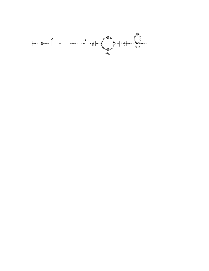
Figure 1: The gluonic “one-loop dressed” contributions to the SDE.

The tree-level expressions for the three- and four-gluon vertices appearing in the two graphs of Fig.(1) are given in the first item of [6]. For the full three-gluon vertex, $\widetilde{{\rm I}\Gamma}$, denoted by the white blob in graph $({a_{1}})$, we employ a gauge technique Ansatz, expressing it as a functional of $\Delta$, in such a way as to satisfy (by construction) the all-order Ward identity

$$q^{\mu}\widetilde{{\rm I}\Gamma}_{\mu\alpha\beta}(q,p_{1},p_{2})=i[{\Delta}^{-1}_{\alpha\beta}(p_{1})-{\Delta}^{-1}_{\alpha\beta}(p_{2})]\,,$$ (1)

characteristic of the PT-BFM. Specifically, we use the following closed form for the vertex [3]:

$$\widetilde{{\rm I}\Gamma}^{\mu\alpha\beta} = \widetilde{\Gamma}^{\mu\alpha\beta}+ig^{\alpha\beta}\,\frac{q^{\mu}}{q^{2}}\,\left[{\Pi}(p_{2})-{\Pi}(p_{1})\right]-i\frac{c_{1}}{q^{2}}\left(q^{\beta}g^{\mu\alpha}-q^{\alpha}g^{\mu\beta}\right)\left[{\Pi}(p_{1})+{\Pi}(p_{2})\right]$$ (2)

$$-ic_{2}\left(q^{\beta}g^{\mu\alpha}-q^{\alpha}g^{\mu\beta}\right)\left[\frac{{\Pi}(p_{1})}{p_{1}^{2}}+\frac{{\Pi}(p_{2})}{p_{2}^{2}}\right]\,.$$

with $\widetilde{\Gamma}_{\mu\alpha\beta}(q,p_{1},p_{2})=(p_{1}-p_{2})_{\mu}g_{\alpha\beta}+2\,q_{\beta}g_{\mu\alpha}-2\,q_{\alpha}g_{\mu\beta}$, and $i\Pi(q^{2})=\Delta^{-1}(q^{2})-q^{2}$.

Defining the renormalization-group invariant quantity [5] ${d}(q^{2})=g^{2}\Delta(q^{2})$, we arrive at

$$d^{-1}(x)=K^{\prime}x+\tilde{b}\sum_{i=1}^{8}{\widehat{A}}_{i}(x)\,+d^{-1}(0)\,,$$ (3)

with

$${\widehat{A}}_{1}(x) = -\left(1+\frac{6c_{2}}{5}\right)x\int_{x}^{\infty}\!\!\!dy\,y\,{\cal L}^{\,2}(y)d^{\,2}(y)\,,$$

$${\widehat{A}}_{2}(x) = \frac{6c_{2}}{5}x\int_{x}^{\infty}\!\!\!dy\,{\cal L}(y)d(y)\,,$$

$${\widehat{A}}_{3}(x) = -\left(1+\frac{6c_{2}}{5}\right)x\,{\cal L}(x)d(x)\int_{0}^{x}\!\!\!dy\,y\,{\cal L}(y)d(y)\,,$$

$${\widehat{A}}_{4}(x) = \left(-\frac{1}{10}-\frac{3c_{2}}{5}+\frac{3c_{1}}{5}\right)\int_{0}^{x}\!\!\!dy\,y^{2}\,{\cal L}^{\,2}(y)d^{\,2}(y)\,,$$

$${\widehat{A}}_{5}(x) = -\frac{6}{5}\bigg{(}1+c_{1}\bigg{)}{\cal L}(x)d(x)\int_{0}^{x}\!\!\!dy\,y^{2}\,{\cal L}(y)d(y)\,,$$

$${\widehat{A}}_{6}(x) = \frac{6c_{2}}{5}\int_{0}^{x}\!\!\!dy\,y\,{\cal L}(y)d(y)\,,$$

$${\widehat{A}}_{7}(x) = \frac{2}{5}\,{\cal L}(x)\,\frac{d(x)}{x}\int_{0}^{x}\!\!\!dy\,y^{3}\,{\cal L}(y)d(y)\,,$$

$${\widehat{A}}_{8}(x) = \frac{1}{5x}\int_{0}^{x}\!\!\!dy\,y^{3}\,{\cal L}^{\,2}(y)d^{\,2}(y)\,,$$ (4)

where $x=q^{2}$. The renormalization constant $K^{\prime}$ is fixed by the condition $d^{-1}(\mu^{2})=\mu^{2}/g^{2}$, (with $\mu^{2}\gg\Lambda^{2}$), and ${\cal L}(q^{2})\equiv\tilde{b}\ln\left(q^{2}/\Lambda^{2}\right)$, where $\Lambda$ is QCD mass scale. Due to the poles contained in the Ansatz for $\widetilde{{\rm I}\Gamma}^{\mu\alpha\beta}$, $d^{\,-1}(0)$ does not vanish, and is given by the (divergent) expression

$$d^{\,-1}(0)=\frac{3\tilde{b}}{5\pi^{2}}\Bigg{[}2(1+c_{1})\int d^{4}k\,{\cal L}(k^{2})\,d(k^{2})-(1+2c_{1})\int\,d^{4}k\,k^{2}\,{\cal L}^{\,2}(k^{2})\,d^{\,2}(k^{2})\Bigg{]}\,,$$ (5)

which can be made finite using dimensional regularization, and assuming that $m^{2}(q^{2})$ drops sufficiently fast in the UV [2].

3 Results

The way to extract from $d(q^{2})$ the corresponding $m^{2}(q^{2})$ and $g^{2}(q^{2})$ is by casting the numerical solutions into the form [1]

$$d(q^{2})=\frac{g^{2}(q^{2})}{q^{2}+m^{2}(q^{2})}\,,\quad g^{2}(q^{2})=\bigg{[}\tilde{b}\ln\left(\frac{q^{2}+f(q^{2},m^{2}(q^{2}))}{\Lambda^{2}}\right)\bigg{]}^{-1}\,.$$ (6)

with

$$f(q^{2},m^{2}(q^{2}))=\rho_{\,1}m^{2}(q^{2})+\rho_{\,2}\frac{m^{4}(q^{2})}{q^{2}+m^{2}(q^{2})}+\rho_{\,3}\frac{m^{6}(q^{2})}{[q^{2}+m^{2}(q^{2})]^{\,2}}\,,$$ (7)

The functional form used for the running mass is

$$m^{2}(q^{2})=\frac{m^{4}_{0}}{q^{2}+m^{2}_{0}}\Bigg{[}\ln\left(\frac{q^{2}+\rho\,m^{2}_{0}}{\Lambda^{2}}\right)\Big{/}\ln\left(\frac{\rho\,m^{2}_{0}}{\Lambda^{2}}\right)\Bigg{]}^{\gamma_{2}-1}\,,$$ (8)

where $\gamma_{2}=\frac{4}{5}+\frac{6c_{1}}{5}$; $\rho$, $\rho_{1}$, $\rho_{2}$, and $\rho_{3}$ are adjustable constants. Evidently, $m^{2}(q^{2})$ is dropping in the deep ultraviolet as an inverse power of the momentum, as expected from general operator-product expansion calculations [7]. Note that $f(q^{2},m^{2}(q^{2}))$ is such that $f(0,m^{2}(0))>0$; as a result, $g^{2}(q^{2})$ reaches a finite positive value at $q^{2}=0$, leading to an infrared fixed point [1, 8, 9].

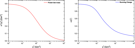
Figure 2: Left: dynamical mass with power-law running, for $m_{0}^{2}=0.5\;\mbox{GeV}^{\,2}$ and $\rho=1.046$ in Eq.(8). Right: the running charge, $\alpha(q^{2})=g^{2}(q^{2})/4\pi$.

3.1 Acknowledgments

This work was supported by the Spanish MEC under the grants FPA 2005-01678 and FPA 2005-00711, and the Fundación General of the University of Valencia.

References

References

[1]
J. M. Cornwall,
Phys. Rev. D 26, 1453 (1982);
J. M. Cornwall and W. S. Hou,
Phys. Rev. D 34, 585 (1986).
[2]
A. C. Aguilar and J. Papavassiliou,
JHEP 0612, 012 (2006).
[3]
A. C. Aguilar and J. Papavassiliou,
arXiv:0708.4320 [hep-ph].
[5]
J. M. Cornwall and J. Papavassiliou,
Phys. Rev. D 40 (1989) 3474;
D. Binosi and J. Papavassiliou,
Phys. Rev. D 66, 111901 (2002);
J. Phys. G 30, 203 (2004).
[6]
L. F. Abbott,
Nucl. Phys. B 185, 189 (1981);
R. B. Sohn,
Nucl. Phys. B 273, 468 (1986);
A. Hadicke,
JENA-N-88-19.
[7]
M. Lavelle,
Phys. Rev. D 44, 26 (1991).
[8]
A. C. Aguilar, A. A. Natale and P. S. Rodrigues da Silva,
Phys. Rev. Lett. 90, 152001 (2003);
A. C. Aguilar, A. Mihara and A. A. Natale,
Phys. Rev. D 65, 054011 (2002);
Int. J. Mod. Phys. A 19 (2004) 249.