Two-dimensional kinematics of SLACS lenses – I. Phase-space analysis of the early-type galaxy SDSS J2321$-$097 at $\mn@boldsymbol{z\approx 0.1}$

Abstract

We present the first results of a combined VLT VIMOS integral-field unit and Hubble Space Telescope (HST)/ACS study of the early-type lens galaxy SDSS J2321$-$097 at $z=0.0819$, extending kinematic studies to a look-back time of 1 Gyr. This system, discovered in the Sloan Lens ACS Survey, has been observed as part of a VLT Large Programme with the goal of obtaining two-dimensional stellar kinematics of 17 early-type galaxies to $z\approx 0.35$ and Keck spectroscopy of an additional dozen lens systems. Bayesian modelling of both the surface brightness distribution of the lensed source and the two-dimensional measurements of velocity and velocity dispersion has allowed us, under the only assumptions of axisymmetry and a two-integral stellar distribution function (DF) for the lens galaxy, to dissect this galaxy in three dimensions and break the classical mass–anisotropy, mass-sheet and inclination–oblateness degeneracies. Our main results are that the galaxy (i) has a total density profile well described by a single power-law $\rho\propto r^{-\gamma^{\prime}}$ with $\gamma^{\prime}=2.06^{+0.03}_{-0.06}$; (ii) is a very slow rotator (specific stellar angular momentum parameter $\lambda_{\mathrm{R}}=0.075$); (iii) shows only mild anisotropy ($\delta\approx 0.15$); and (iv) has a dark-matter contribution of $\sim 30$ per cent inside the effective radius. Our first results from this large combined imaging and spectroscopic effort with the VLT, Keck and HST show that the structure of massive early-type galaxies beyond the local Universe can now be studied in great detail using the combination of stellar kinematics and gravitational lensing. Extending these studies to look-back times where evolutionary effects become measurable holds great promise for the understanding of formation and evolution of early-type galaxies.

1 Introduction

Within the hierarchical galaxy formation scenario, early-type galaxies are assumed to be the end-products of major mergers with additional accretion of smaller galaxies (e.g. Burkert & Naab 2004 for a review). As such the study of their structure, formation and evolution is an essential step in understanding galaxy formation and the standard $\Lambda$ cold dark matter ($\Lambda$CDM) paradigm, in which the hierarchical galaxy formation model has its foundations. Early-type galaxies are observed to follow tight scaling relations between their stellar population, dark matter, kinematic and black hole properties, the origins of which are still not well understood (e.g. Djorgovski & Davis, 1987; Dressler et al., 1987; Magorrian et al., 1998; Bolton et al., 2007).

Considerable observational progress has been made in the last decades in our understanding of the relative contributions of baryonic (mostly stellar), dark matter and black hole constituents of early-type galaxies through stellar dynamical tracers and X-ray studies (e.g. Fabbiano 1989; Mould et al. 1990; Saglia, Bertin, & Stiavelli 1992; Bertin et al. 1994; Franx, van Gorkom, & de Zeeuw 1994; Carollo et al. 1995; Arnaboldi et al. 1996; Rix et al. 1997; Matsushita et al. 1998; Loewenstein & White 1999; Gerhard et al. 2001; Seljak 2002; Borriello, Salucci, & Danese 2003; Romanowsky et al. 2003). More recently, the SAURON collaboration (de Zeeuw et al., 2002) has extensively studied a large and uniform sample of early-type galaxies in the local Universe (i.e. $z\la 0.01$), combining SAURON integral-field spectroscopy (IFS) on the William Herschel Telescope with high-resolution Hubble Space Telescope (HST) imaging to obtain a three-dimensional picture of these galaxies in terms of their mass and kinematic structure (Emsellem et al., 2004, 2007; Cappellari et al., 2006, 2007).

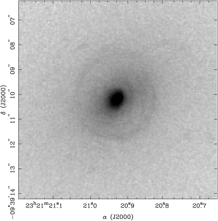
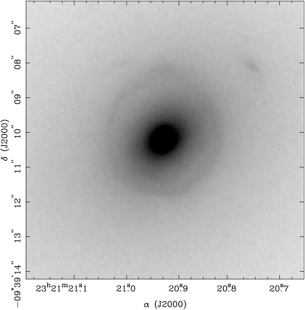
Figure 1: HST/ACS images of SDSS J2321$-$097, taken through the F435W (left-hand panel) and F814W (right-hand panel) filters. The images are single exposures with an integration time of $420\,\mathrm{s}$; the pixel scale is $0.05\,\mathrm{arcsec}$. A full description of these observations and the data-reduction process is given in Bolton et al. (2006).

Despite making a great leap forward, the complex modelling of the SAURON systems and the unknown dark matter content and total mass of these galaxies still require some assumptions to be made about their gravitational potential [e.g. constant stellar mass-to-light ratio ($M/L$) from stellar population models] and inclination. These issues can be partly overcome in discy systems where the inclination can be determined from the photometry or possibly from dust lanes. However, systems with lower ellipticity can show stronger degeneracies (e.g. Cappellari et al., 2007). Also, near the effective radius dark matter becomes a major contributor to the stellar kinematics (Gerhard et al., 2001; Treu & Koopmans, 2004) and it is not yet clear what impact its neglect has, even though it is estimated to be not too severe (Cappellari et al., 2006).

At higher redshifts, the extraction of detailed kinematic information from early-type galaxies becomes increasingly more difficult because of the decrease in apparent size and cosmological surface brightness dimming. However, galaxies at higher redshifts are much more likely to act as gravitational lenses on background galaxies (e.g. Turner, Ostriker, & Gott, 1984). The additional information obtained from gravitational lensing on, for example, the enclosed mass and the density profile has been shown to break some of the classical degeneracies in stellar kinematics and lensing, namely the mass–anisotropy and the mass-sheet degeneracies, respectively (e.g. Treu & Koopmans, 2002a; Koopmans et al., 2003; Koopmans & Treu, 2003; Treu & Koopmans, 2004; Koopmans et al., 2006; Barnabè & Koopmans, 2007, hereafter BK07).

In order to use gravitational lensing and stellar dynamics in a systematic way, the Lenses Structure & Dynamics (LSD) Survey was started in 2001, combining HST imaging data on lens systems with stellar kinematics obtained with Keck (Koopmans & Treu, 2002, 2003; Treu & Koopmans, 2002a, b, 2003, 2004). This project and its results, predominantly at $z\approx 0.5\!\!-\!\!1.0$, have shown the validity of this methodology and its effectiveness at higher redshifts. These high-redshift systems, however, are relatively rare and hard to follow up, which has limited studies to the use of luminosity-weighted stellar velocity dispersions (e.g. Koopmans & Treu, 2002; Treu & Koopmans, 2002b) or long-slit spectroscopy in a few large apertures along the major axes (e.g. Koopmans & Treu, 2003; Treu & Koopmans, 2004).

The Sloan Lens ACS Survey (SLACS, Bolton et al., 2005, 2006) was begun to extend the sample of lens galaxies suitable for joint lensing and dynamical studies. SLACS lens candidates were selected from the SDSS Luminous Red Galaxy sample (Eisenstein et al., 2001) and a quiescent subsample [defined by $\mathit{EW}(\mathrm{H}\alpha)<1.5\,$Å] of the MAIN SDSS galaxy sample (Strauss et al., 2002) by an inspection of their SDSS fibre spectroscopy (Bolton et al., 2004). Galaxies whose spectra presented emission lines at a higher redshift than the redshift of the galaxy itself were observed in an HST snapshot programme to check whether the source of the emission lines was a gravitationally lensed background galaxy. To date, SLACS has confirmed around 80 lens systems (Bolton et al., in preparation). In contrast to most earlier lens surveys which drew their candidate systems from catalogues of potential sources (e.g. quasi-stellar objects or radio sources as in the CLASS survey, Browne et al., 2003), SLACS is a lens-selected survey and as such preferentially finds systems with bright lens galaxies but comparatively faint sources. It is therefore an ideal starting point for detailed investigations into the properties of the lens galaxies.

In this paper we introduce a follow-up project to SLACS which aims at combining the lensing information with detailed two-dimensional kinematic information obtained with the VIMOS integral-field unit (IFU) mounted on the VLT. The full sample comprises 17 systems. In this paper we demonstrate the available data and the analysis methodology on one system, SDSS J2321$-$097. The lens in this system is an early-type galaxy at $z=0.0819$. The SDSS spectrum shows additional [O ii] and H$\beta$ emission from a gravitationally lensed blue galaxy at $z_{\mathrm{s}}=0.5342$ (Bolton et al., 2006). In HST imaging (Fig. 1) the lensed source is shown to form an almost complete Einstein ring of radius $1.68\,\mathrm{arcsec}$, corresponding to an Einstein radius of $R_{\mathrm{Einst}}=2.6\,\mathrm{kpc}$ at the lens redshift. The projected mass enclosed within the Einstein radius is $M(<R_{\mathrm{Einst}})=1.3\times 10^{11}\,M_{\sun}$. Details on this system are listed in Table 1.

In Section 2, we describe the VIMOS and HST observations that form the basis of this analysis. The IFU data are presented in Section 3, with a description of the data reduction in Section 3.1 and of the extraction of two-dimensional kinematic maps in Section 3.2. In Section 3.3 we determine several commonly used parameters from the kinematic data alone, in a way that is directly comparable to earlier studies, for example from the SAURON collaboration. We apply the joint lensing and dynamics analysis developed by BK07 in Section 4. In Section 5 we present a physical argument that explains why gravitational lensing and stellar dynamics can break the degeneracy between oblateness and inclination. We discuss our results and conclude in Section 6. We use a concordance $\Lambda$CDM model throughout this paper, described by $\Omega_{\mathrm{M}}=0.3$, $\Omega_{\Lambda}=0.7$ and $H_{0}=100\,h\,\mathrm{km\,s^{-1}\,Mpc^{-1}}$ with $h=0.7$ unless stated otherwise. At the redshift of SDSS J2321$-$097, $1\,\mathrm{arcsec}$ corresponds to $1.1\,h^{-1}\,\mathrm{kpc}=1.5\,\mathrm{kpc}$.

Table 1: Basic data for SDSS J2321$-$097. The data are taken from Treu et al. (2006a) and Koopmans et al. (2006).

$\alpha_{\mathrm{J2000}}$	$23^{\mathrm{h}}21^{\mathrm{m}}20\aas@@fstack{s}93$
$\delta_{\mathrm{J2000}}$	$-09\degr 39\arcmin 10\aas@@fstack{\prime\prime}2$
$z_{\mathrm{l}}$	$0.0819$
$z_{\mathrm{s}}$	$0.5342$
$\sigma_{\mathrm{ap}}$	$(236\pm 7)$	$\mathrm{km\,s^{-1}}$
$\sigma_{\mathrm{c}}$	$(245\pm 7)$	$\mathrm{km\,s^{-1}}$
$R_{\mathrm{Einst}}$	$1.68\,\mathrm{arcsec}=2.59$	$\mathrm{kpc}$
$R_{\mathrm{eff},B}$	$(8.47\pm 0.11)$	$\mathrm{kpc}$
$M_{B}$	$-21.72\pm 0.05$
$R_{\mathrm{eff},V}$	$(7.93\pm 0.07)$	$\mathrm{kpc}$
$M_{V}$	$-22.59\pm 0.05$
$q_{\mathrm{iso,2D}}$	$0.77$
$\vartheta_{\mathrm{PA},\star}$	$126\aas@@fstack{\circ}5$

Notes: $z_{\mathrm{l}}$ and $z_{\mathrm{s}}$ are the redshifts of SDSS J2321$-$097 and the gravitationally lensed background galaxy, respectively. $\sigma_{\mathrm{ap}}$ is the velocity dispersion measured from the 3-arcsec-diameter SDSS fibre, $\sigma_{\mathrm{c}}$ is the derived central velocity dispersion (Treu et al., 2006b). $R_{\mathrm{Einst}}$ is the Einstein radius. $R_{\mathrm{eff}}$ and $M$ are the effective radii and absolute magnitudes determined by fitting de Vaucouleurs profiles to the $B$- and $V$-band ACS images (Treu et al., 2006b). $q_{\mathrm{iso,2D}}$ and $\vartheta_{\mathrm{PA},\star}$ are isophotal axial ratio and position angle of the major axis, respectively (Koopmans et al., 2006).

2 Observations

In this section, we briefly discuss the VLT VIMOS/IFU spectroscopic and the HST imaging observations, which form the basic data sets for the subsequent modelling.

2.1 Integral-field spectroscopy

We have obtained integral-field spectroscopic observations of 17 systems using the IFU of VIMOS (Le Fèvre et al., 2001) mounted on the VLT UT3 (Melipal). The observations were conducted in two parts: three systems were observed in a pilot programme (ESO programme 075.B-0226; PI: Koopmans) and the remaining 14 systems in a large programme (177.B-0682; PI: Koopmans) with a slightly different observational setup. Observations were carried out in service mode throughout to ensure uniform observing conditions. In this paper we report in detail on the observations of the pilot programme and the analysis of one system, SDSS J2321$-$097. The observations of the large programme and the analysis of the full sample will be presented in forthcoming papers in this series.

The IFU head of VIMOS consists of a square array of $80\times 80$ microlenses with a sampling of $0.67\,\mathrm{arcsec}$ per spatial element (‘spaxel’) at the Nasmyth focus of the telescope. In high-resolution mode only the central 1600 lenses are used, resulting in a field of view of $27\times 27\,\mathrm{arcsec^{2}}$. The lenses are coupled to optical fibres which transmit the light to pseudo-slit masks, each of which contains 400 fibres and corresponds to a quadrant of the original field. The seeing limit for the observations was set to $0.8\,\mathrm{arcsec}$, so that each fibre of the IFU gives a spectrum that is essentially independent of its neighbours.

For the pilot programme, we employed the HR-Blue grism which covers a wavelength range from $4000$ to $6200$ Å (the exact wavelength range varies slightly from quadrant to quadrant). The spectral resolution of the HR-Blue grism is $\lambda/\Delta\lambda=2550$, where $\Delta\lambda$ is the full width at half-maximum (FWHM) of the instrument profile. The mean dispersion on the CCD is $0.5$ Å per pixel. Three exposures of $555\,\mathrm{s}$ integration time were obtained per observing block (a one-hour sequence of science and calibration exposures); the telescope was shifted by about $3.5\,\mathrm{arcsec}$ between the exposures to fill in on dead fibres. The number of observing blocks spent on each lens system was adjusted so as to reach approximately equal signal-to-noise ratios ($S/N$) across the sample. For the system described in this paper, SDSS J2321$-$097, five observing blocks were carried out for a total integration time of $8325\,\mathrm{s}$. For the large programme, we switched to the HR-Orange grism which covers a wavelength range from $5250$ to $7400$ Å at a similar spectral resolution of $\lambda/\Delta\lambda=2650$ and a dispersion of $0.6$ Å per pixel. The spectral resolution translates to a rest-frame velocity resolution $\Delta v$ varying between $107$ and $85\,\mathrm{km\,s^{-1}}$, improving as the redshift of our sample lens galaxies increases from $0.08$ to $0.35$.

2.2 HST imaging

High-resolution imaging with HST/ACS or HST/WFPC2 has been or is being obtained for all confirmed SLACS lenses (Bolton et al., 2006; Gavazzi et al., 2007). The data used here come from the ACS snapshot survey described by Bolton et al. (2005) and consist of single $420\,\mathrm{s}$ exposures through the F435W and F814W filters, respectively. Fig. 1 shows the images of SDSS J2321$-$097. The lens modelling requires as input a clean estimate of the brightness distribution of the lensed images, so the smooth brightness distribution of the lens galaxy has to be subtracted from the images. Bolton et al. (2006) tried a variety of commonly used modelling techniques (e.g. fitting of Sersic profiles), but settled on the more flexible B-spline technique. The galaxy-subtracted image in the F814W filter is shown in the top right-hand panel of Fig. 7.

3 IFU data analysis

3.1 Data reduction

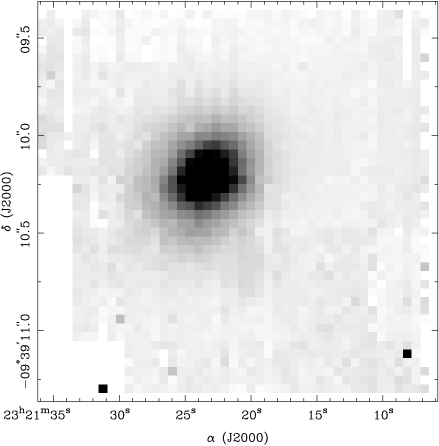
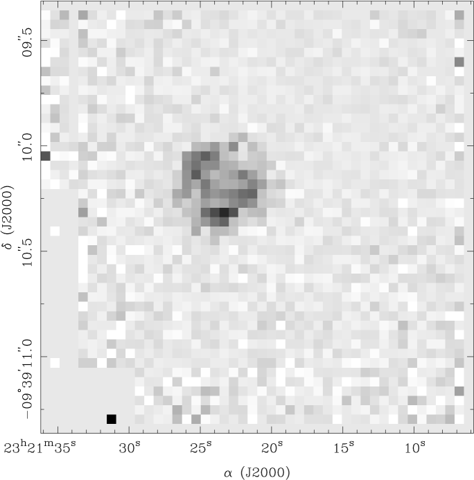
Figure 2: Left-hand panel: VLT VIMOS/IFU image reconstruction of SDSS J2321$-$097, obtained by integrating along the individual fibre spectra from 4400 to 6100 Å. Right-hand panel: map of the strength of the [O ii] doublet from the lensed source.

The VLT VIMOS/IFU data were reduced using the vipgi package which was developed within the framework of the VIRMOS consortium and the VVDS project. vipgi has been described in detail by Scodeggio et al. (2005) and Zanichelli et al. (2005); here, we restrict ourselves to a brief summary of the main reduction steps performed by vipgi.

The four quadrants of the IFU are treated independently up to the combination of all exposures into the final data cube. For each night on which observations were carried out, five bias exposures were obtained which are median-combined and subtracted from the data. The observed halogen-lamp illuminated screen flats are used to locate the traces of the individual spectra on the CCD, starting from interactively adjusted first guesses of the layout of the fibres. This includes a shift correction and an identification of ‘bad’ fibres. The position of the peak of each spectrum in the spatial direction is then modelled as a quadratic polynomial function of the position in the dispersion direction. vipgi does not perform a CCD pixel-to-pixel flat-field correction (Scodeggio et al., 2005).

The wavelength calibration is subsequently done using helium and neon lamp observations taken immediately after the science exposures. With about 20 lines spread between $\sim 4000$ and $\sim 6200$ Å, the rms deviations from the polynomial fit are roughly Gaussian-distributed around a mean of $\sim 0.075$ Å and a dispersion of $\sim 0.02$ Å. The velocity error introduced by uncertainties in the wavelength calibration is thus of the order of $5\,\mathrm{km\,s^{-1}}$, significantly smaller than the spectral resolution and negligible in our analysis.

Figure 3: Spectrum of SDSS J2321$-$097 integrated from the VIMOS/IFU data cube over a circular aperture of diameter $3\,\mathrm{arcsec}$. The inset on the right-hand side shows a zoom on the [O ii] doublet of the lensed background galaxy at $z_{\mathrm{s}}=0.5342$, next to the FeCa $\lambda 5268$ line of the lens. The inset on the left-hand side shows a zoom on the weak but clearly detected [O ii] line of the lens galaxy. Several other spectral features of the lens are marked.

The individual spectra are extracted using the optimal extraction scheme of Horne (1986), that is, by averaging the flux across the spectral trace of the fibre, weighted by a fit to its spatial profile. In order to correct for the transmissivity variations from fibre to fibre (‘spaxel-to-spaxel flat-fielding’), the flux under a sky emission line is measured and scaled relative to a reference fibre. We use [O i] at $\lambda=5577$ Å for this purpose.

Spectrophotometric standard stars were observed during most nights. Since the stellar light only covers a small fraction of the fibres in the IFU field whereas the calibration is applied to all fibres, the spectrophotometric calibration only accurately corrects the relative wavelength dependence of the sensitivity function (assuming that this is the same for all fibres), while the absolute flux levels are determined with a much larger uncertainty due to residuals from the correction of the varying fibre transmissivities.

The VIMOS IFU does not have dedicated sky fibres, but the field of view is large enough for a sufficient number of fibres to essentially measure pure sky. vipgi identifies these fibres in a statistical way by integrating the flux in each fibre over a large wavelength range and selecting as sky fibres those with a flux within $\pm 0.1$ per cent of the mode of the resulting distribution.

Finally, the four quadrants of all the individual exposures are combined into a single data ‘cube’ after correction for the dithering between exposures. The final data are in row-stacked form, where each row corresponds to the spectrum from one fibre. A fits table extension gives the translation from row number to the spatial coordinate of the fibre.

The left-hand panel of Fig. 2 shows an image of SDSS J2321$-$097, reconstructed from the reduced data cube using the program sadio by integrating along the wavelength direction from $4400$ to $6100\,$Å. The galaxy surface brightness distribution agrees well with that seen in the HST/ACS F435W and F814W snapshot images, although it is not as precise due to the complexities involved in the spectral calibration, in particular of the relative fibre transmissivity. In the modelling of the lens galaxy brightness distribution, we therefore use the HST images. The imperfect absolute flux calibration of the IFU data has no effect on the measurements of the stellar kinematics which do not depend on the overall scaling of each fibre spectrum.

Following Bolton & Burles (2007), we can use the IFU data to obtain an image of the lensed source by isolating its redshifted [O ii] emission line at $5710\,$Å. The [O ii] doublet is modelled as the sum of two Gaussians with separation $4.5$ Å (taking into account the redshift of the source) and relative strength 3:2. In regions with significant light from the lens galaxy the best-fitting kinematic model (Section 3.2) was subtracted prior to the fit; elsewhere a polynomial fit was subtracted to remove a remaining continuum level. The map of the line strength of the [O ii] line obtained in this manner is presented in the right-hand panel panel of Fig. 2. The map clearly shows the ring-like structure of the lensed galaxy (cf. the higher resolution galaxy-subtracted ACS image in the top right-hand panel of Fig. 7) and demonstrates that the [O ii] line used for the inclusion of this system in the SLACS sample indeed originates from a gravitationally lensed background galaxy.

The spectral energy distribution of SDSS J2321$-$097 is essentially that of a typical early-type galaxy with strong metal lines, as seen in Fig. 3 which shows the spectrum integrated over a circular aperture of $3\,\mathrm{arcsec}$ diameter (i.e. the SDSS aperture). We note, however, that this spectrum shows weak but significant [O ii] emission ($\mathrm{EW}\sim-4\,$Å) as well as H$\delta$ absorption from the lens galaxy. This might indicate residual star formation or active galactic nucleus activity at a low level.

3.2 Kinematic analysis

We extract two-dimensional maps of systematic velocity $v(\mn@boldsymbol{R})$ and line-of-sight velocity dispersion $\sigma(\mn@boldsymbol{R})$ using a direct pixel-fitting method implemented in the statistical language r (R Development Core Team, 2007). Since the analysis is done on spectra from individual IFU fibres, the spectra have relatively low signal-to-noise ratio, in particular in the outskirts of the lens galaxy where the surface brightness drops rapidly. We therefore restrict the model to a Gaussian line-of-sight velocity distribution (LOSVD) and do not attempt to measure higher order moments, such as the Gauss–Hermite coefficients $h_{3}$ and $h_{4}$ commonly used in kinematic studies of low-redshift early-type galaxies (e.g. van der Marel & Franx, 1993; Cappellari & Emsellem, 2004).

The observed galaxy spectrum $d_{i}(\lambda)$ is modelled, for each fibre $i$ separately, by the convolution of a high-resolution stellar template spectrum $t(\ln\lambda)$ with a Gaussian kernel $g_{i}(\ln\lambda)$ with dispersion $\sigma_{v,i}/c$:

$$d_{i}(\lambda)=f_{i}(\lambda)\,[t\otimes g_{i}](\ln\lambda)+n_{i}(\lambda)\;.$$ (1)

We assume Gaussian noise $n(\lambda)$ on the spectrum. Since the accuracy of the spectrophotometric calibration is not perfect for both our spectra and the chosen template spectra (see below and Valdes et al., 2004) there remain small relative tilts between the continua of the galaxy and template spectra. We model this difference by the linear correction function $f(\lambda)=a+b\lambda$ whose parameters are determined by a linear fit nested within the non-linear optimization for the kinematic parameters $v_{i}$ and $\sigma_{v,i}$.

The template spectrum is first resampled to a logarithmic wavelength scale with step $\Delta\ln\lambda=\Delta v/c$, where we use a velocity step of $\Delta v=25\,\mathrm{km\,s^{-1}}$. The convolution kernel is a Gaussian with dispersion $\sigma_{\mathrm{G}}=\sigma_{v}/\Delta v$, extending to $\pm 8\sigma_{\mathrm{G}}$. The galaxy spectrum is corrected for the mean redshift of the lens galaxy, $z=0.0819$ in the case of SDSS J2321$-$097, taken from the SDSS data base. The model is then resampled on to the wavelength grid of the galaxy spectrum, a linear wavelength scale $\lambda_{\mathrm{obs}}/(1+z_{\mathrm{SDSS}})$ in our case. This avoids further resampling of the data beyond what was done in the data reduction. Similar methods typically resample both model and data to the same logarithmic wavelength grid before comparing (e.g. van der Marel, 1994; Cappellari & Emsellem, 2004).

Remaining cosmic rays, emission lines, and remnants of sky lines are masked automatically by $3\sigma$-clipping of the residuals from a preliminary fit without mask. Fig. 4 shows an example of a fit to a spectrum from a fibre near the centre of SDSS J2321$-$097. Error analysis is performed through a Monte Carlo technique by adding Gaussian noise to the best-fitting model at the noise level given by the residuals between model and data, and using 1000 realizations to determine the spread of the best-fitting parameters.

The choice of a good template spectrum is important for accurate kinematic measurements from galaxy spectra. For SDSS J2321$-$097, we started by experimenting with a set of eight stellar template spectra obtained with the Echelle Spectrograph and Imager (ESI) on the Keck II telescope (Koopmans & Treu, 2002) applied to the global spectrum of SDSS J2321$-$097. These spectra have a velocity resolution of $\Delta v_{\mathrm{ESI}}=22.4\,\mathrm{km\,s^{-1}}$ (ESI manual) and cover a range of spectral types G0 to K4, luminosity class III. Fitting to the integrated spectrum of SDSS J2321$-$097 it was found that four templates for stellar types between G7 and K0 gave consistent results for the velocity dispersion within $\pm 10\,\mathrm{km\,s^{-1}}$, which also agreed with the measurement from the SDSS. Cooler template stars (K2 and K4) resulted in a significantly higher velocity dispersion while hotter templates (G0 and G5) gave lower values. On the basis of the visual appearance of the fit and the shape of the galaxy spectrum it was decided to use the K0 star HR 19 as the template star for SDSS J2321$-$097.

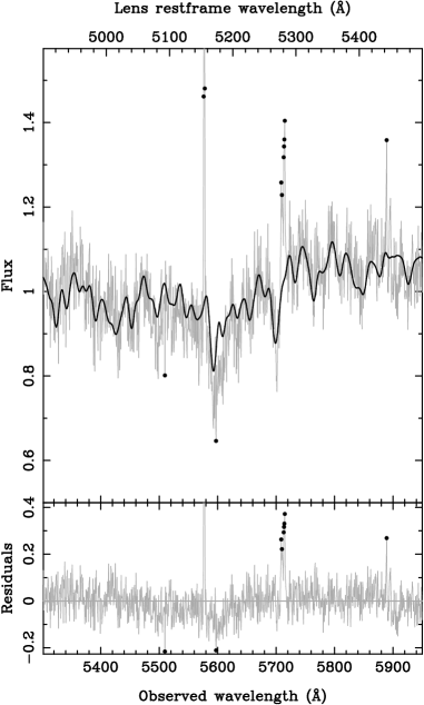
Figure 4: Spectrum from a single fibre near the centre of SDSS J2321$-$097, with the overlaid best-fitting model (top panel). The bottom panel shows the residuals of the fit. The [O ii] doublet from the source at $5710\,$Å ($z_{\mathrm{s}}=0.5342$) and the residual of the [O i] sky line at $5577\,$Å were masked automatically (indicated by the points).

We subsequently exchanged the ESI spectrum of HR 19 for the corresponding spectrum from the Indo-US library of Coudé feed stellar spectra (Valdes et al., 2004). The Indo-US library contains spectra for 1273 stars covering a wide range of stellar parameters. The spectra have a resolution of $\sim 1\,$Å FWHM and for the majority of stars cover a wavelength range of $3460$ to $9464$ Å. While the resolution of the Indo-US spectra is somewhat lower than that of the ESI spectra, this disadvantage is offset by the large number of spectra available, which will provide freedom of choice for the analysis of our full sample. We have checked that the kinematic results obtained with the Indo-US and the ESI templates are indeed consistent.

Fig. 4 shows an important limitation of any use of observed stellar spectra as templates in kinematic analyses, namely the differing abundance ratios between stars in the solar neighbourhood and early-type galaxies (Barth, Ho, & Sargent, 2002). While the strengths of the Fe i/Ca i $\lambda 5268$ lines agree, the Mg $b$ $\lambda 5174$ line is significantly enhanced in the galaxy spectrum. Barth et al. (2002) recommend masking the Mg $b$ line before fitting. Doing this increases the velocity dispersion only by a few per cent and does not significantly improve the fit outside the Mg $b$ region.

3.3 Results from the observed stellar kinematics

A fit of a kinematic model to the global spectrum (Fig. 3) following the procedure described in Section 3.2 results in a velocity dispersion of $\sigma_{\mathrm{tot}}=240\pm 8\,\mathrm{km\,s^{-1}}$, which is consistent with the value $\sigma_{\mathrm{SDSS}}=236\pm 7\,\mathrm{km\,s^{-1}}$ listed in the SDSS data base (Bolton et al., 2006). Note that the error estimates are not directly comparable because of differences in the estimation method. We believe our Monte Carlo estimate to be more reliable, although it might still underestimate the real error due to the assumption of Gaussian noise in the spectrum (de Bruyne et al., 2003).

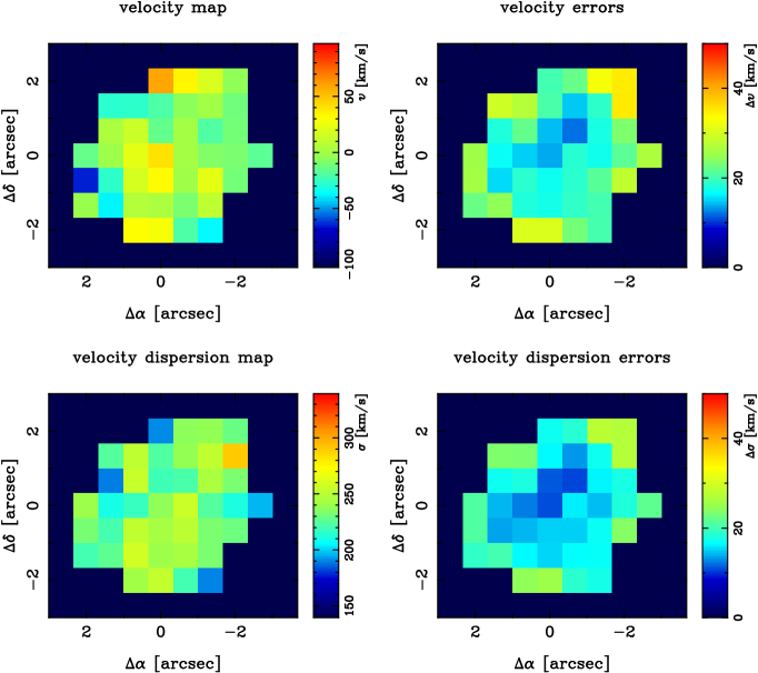
Figure 5: Kinematic maps of SDSS J2321$-$097. The top left-hand panel shows systematic velocity relative to the mean redshift of the lens galaxy; the bottom left-hand panel shows the velocity dispersion. The panels on the right-hand side visualize the corresponding $1\sigma$ errors on the measurements. Spaxel size is $0.67\,\mathrm{arcsec}$ and only spectra with $S/N>8$ were analysed.

The two-dimensional maps of the velocity and velocity dispersion are shown in Fig. 5. Only fibres in which the spectrum has an $S/N$ per pixel in the rest-frame wavelength range from 5350 Å to 5450 Å (a flat part of the spectrum) of $S/N>8$ are used in these maps and the subsequent analysis. Spectra with lower $S/N$ were found not to yield reliable kinematic fits.

Neither the velocity nor the velocity dispersion map shows significant structure. The velocity map might hint at a pattern of slight rotation, although within the noise the map is consistent with no rotation at all.

In order to quantify the amount of rotation in a galaxy from two-dimensional maps of line-of-sight stellar velocity $v$ and velocity dispersion $\sigma_{v}$, Emsellem et al. (2007) defined a stellar angular momentum parameter $\lambda_{\mathrm{R}}$ by

$$\lambda_{\mathrm{R}}=\frac{\langle R\,|v|\rangle}{\langle R\sqrt{v^{2}+\sigma_{v}^{2}}\rangle}\;,$$ (2)

where $R$ is the projected distance from the galaxy centre. We find $\lambda_{\mathrm{R}}=0.075$, which in combination with the absolute magnitude $M_{B}=-21.72$ places SDSS J2321$-$097 among the slowly rotating galaxies at the high-luminosity end of the SAURON sample (cf. fig. 7 of Emsellem et al., 2007).

Following the prescription of Binney (2005) and Cappellari et al. (2007), we find a low value for the ratio between systematic velocity and velocity dispersion of $(\langle v^{2}\rangle/\langle\sigma_{v}^{2}\rangle)^{1/2}=0.1$, which in combination with the observed ellipticity of $\epsilon_{\mathrm{iso,2D}}=1-q_{\mathrm{iso,2D}}=0.23$ from isophote fitting places SDSS J2321$-$097 well below the curve for an isotropic rotating oblate galaxy in an $\epsilon\!\!-\!\!(v/\sigma_{v})$ diagram. From the tensor virial theorem the global anisotropy parameter (Binney, 2005) is found to be $\delta\sim 0.15$, where no correction for inclination has been made yet. In Section 4, we calculate the same quantity from the reconstructed stellar DF and find effectively the same result. Again, SDSS J2321$-$097 compares well with the high-luminosity galaxies from the SAURON sample (Cappellari et al., 2007) in that its ellipticity requires an anisotropic velocity distribution and is not due to rotation.

Figure 6: Velocity (top panels) and velocity dispersion (bottom panels) as a function of position along the major (left-hand panels) and minor (right-hand panels) axes. Spectra from fibres within $1\,$arcsec of the respective axis were used here.

The velocity dispersion is nearly constant across the field as one would expect for a nearly isothermal total mass distribution. Fig. 6 shows the velocity and velocity dispersion as a function of position along the major and minor axes (fibres within $1\,\mathrm{arcsec}$ of the respective axis were used). The major axis velocity cut shows a hint of the S-shape expected from rotation around the minor axis, although at a very low level. The velocity dispersion along the major axis is perfectly flat, whereas the minor axis cut shows a slight decline outwards.

To quantify this, we perform a linear fit to the velocity dispersion profile as a function of the elliptical radius $\mu^{2}=x^{2}+y^{2}/q_{\mathrm{iso,2D}}^{2}$, with $q_{\mathrm{iso,2D}}=0.77$ obtained by ellipse fitting to the light distribution. The linear slope is $\mathrm{d}\sigma/\mathrm{d}\mu=(-7.3\pm 4.5)\,\mathrm{km\,s^{-1}\,arcsec^{-1}}$, consistent with being fully isothermal.

4 Joint self-consistent gravitational lensing and stellar dynamics analysis

In this section, we combine the information from the gravitationally lensed image with the surface brightness distribution from HST observations and the projected velocity moment maps derived from VLT observations of the lens galaxy SDSS J2321$-$097 in order to constrain the total mass density profile of this galaxy. The analysis is carried out by making use of the cauldron algorithm, presented in BK07: we refer to that paper for a detailed description of the method.

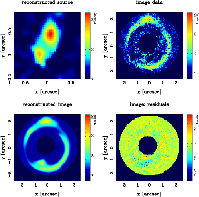
Figure 7: Best model lens image reconstruction for the system SDSS J2321$-$097. From the top left-hand to bottom right-hand panel: reconstructed source model; HST/ACS data showing the lensed image after subtraction of the lens galaxy; lensed image reconstruction; residuals.

4.1 Mass model and overview of the joint analysis

The key idea of a self-consistent joint analysis is to adopt the same total gravitational potential $\Phi$ for both the gravitational lensing and the stellar dynamics modelling of the data. As shown in BK07, these two modelling problems, although different from a physical point of view, can be expressed in an analogous way as a single set of coupled (regularized) linear equations. For any given choice $\mn@boldsymbol{\eta}$ of the non-linear potential parameters, the equations can be solved non-iteratively to simultaneously obtain as the best solution for the chosen potential model the unlensed source surface brightness distributions and the weights of the elementary stellar dynamics building blocks (e.g. orbits or two-integral components, TICs, Schwarzschild, 1979; Verolme & de Zeeuw, 2002). This linear optimization scheme is consistently embedded in the framework of Bayesian statistics. As a consequence, it is possible to objectively assess the probability of each model by means of the evidence merit function and, therefore, to rank different models (see MacKay, 1992, 1999, 2003). In this way, by maximizing the evidence, the set of non-linear parameters $\mn@boldsymbol{\eta}$ which corresponds to the best potential model, given the data, can be recovered.

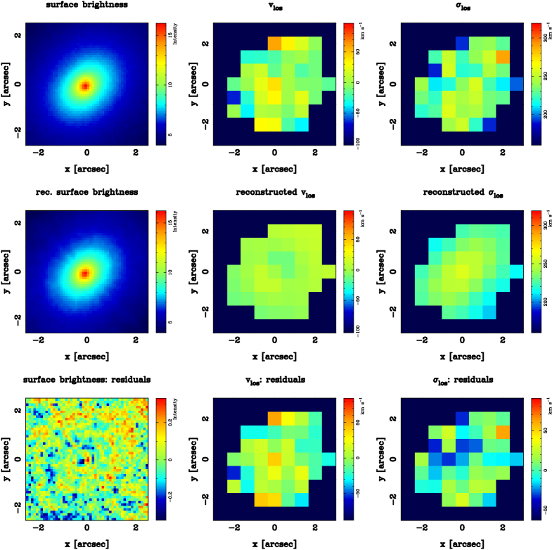
Figure 8: Best dynamical model for the galaxy SDSS J2321$-$097. First row: observed surface brightness distribution, projected line-of-sight velocity and line-of-sight velocity dispersion. Second row: corresponding reconstructed quantities for the best model. Third row: residuals. The low-level ripples in the surface brightness residuals are due to the discrete nature of the TICs.

While the method is completely general, its practical implementation (in the cauldron algorithm) is more restricted to make it computationally efficient and applies specifically to axisymmetric potentials, $\Phi(R,z)$, and two-integral DFs $f=f(E,L_{z})$. Under these assumptions, the dynamical model can be constructed by making use of the fast BK07 numerical implementation of the two-integral Schwarzschild method developed by Cretton et al. (1999) and Verolme & de Zeeuw (2002), whose building blocks are not orbits (as in the classical Schwarzschild method) but TICs. Among the outcomes of the joint analysis presented in this section is the weights map of the TIC superposition, which can be related to the weighted two-integral DF (see BK07).

As a first-order model and in order to allow a straightforward comparison with the results of the preliminary analysis of Koopmans et al. (2006), we adopt as the total mass density distribution of the galaxy a power law stratified on axisymmetric homoeoids:

$$\rho(m)=\frac{\rho_{0}}{m^{\gamma^{\prime}}},\quad 0<\gamma^{\prime}<3,$$ (3)

where $\rho_{0}$ is a density scale, $\gamma^{\prime}$ will be referred to as the (logarithmic) slope of the density profile, and

$$m^{2}=\frac{R^{2}}{a^{2}}+\frac{z^{2}}{c^{2}}=\frac{R^{2}}{a^{2}}+\frac{z^{2}}{a^{2}q^{2}},$$ (4)

with $a\geq c$ and $c/a\equiv q$.

The (inner) gravitational potential associated with a homoeoidal density distribution $\rho(m)$ is given by Chandrasekhar’s formula (Chandrasekhar 1969; see also e.g. Merritt & Fridman 1996 and Ciotti & Bertin 2005). We find, for $\gamma^{\prime}\neq 2$,

$$\Phi(R,z)=-\Phi_{0}\int_{0}^{+\infty}\frac{[1/(\gamma^{\prime}-2)]\,{\tilde{m}}^{2-\gamma^{\prime}}}{(1+\tau)\sqrt{q^{2}+\tau}}\,\mathrm{d}\tau\;,$$ (5)

where $\Phi_{0}=2\pi Gqa^{2}\rho_{0}$ and

$$\tilde{m}^{2}=\frac{R^{2}}{a^{2}(1+\tau)}+\frac{z^{2}}{a^{2}(q^{2}+\tau)}.$$ (6)

For $\gamma^{\prime}=2$ we have

$$\Phi(R,z)=-\Phi_{0}\int_{0}^{+\infty}\frac{\log(1/\tilde{m})}{(1+\tau)\sqrt{q^{2}+\tau}}\,\mathrm{d}\tau.$$ (7)

There are three free non-linear parameters in the potential to be determined via the evidence maximization: $\Phi_{0}$ (or equivalently, through equation [B4] of BK07, the lens strength $\alpha_{0}$), the slope $\gamma^{\prime}$ and the axial ratio $q$. One can also easily include a core radius $R_{\mathrm{s}}$ by modifying the definition of the homoeoidal radius $m$, but for the purpose of the present analysis it was kept fixed to a negligibly small value. In addition to the previously mentioned parameters, there are four additional parameters which determine the geometry of the observed system: the position angle $\vartheta_{\mathrm{PA}}$, the inclination $i$ and the coordinates of the centre of the lens galaxy with respect to the sky grid.

The cauldron algorithm is run on the data sets (and the corresponding covariance matrices) described in the previous sections.

1. The lensed image surface brightness distribution is defined on a $100\times 100$ grid ($1~{}\mathrm{pixel}=0.05\,\mathrm{arcsec}$) on which the innermost and outermost low-$S/N$ regions have been masked out, and the source is reconstructed on a $40\times 40$ grid. To include the effects of seeing in the modelling, the lensing matrix is blurred with a blurring operator which takes into account the HST/ACS F814W point spread function (PSF) obtained with tiny tim (Krist, 1993).

2. The lens galaxy surface brightness distribution is given on a $50\times 50$ grid ($1~{}\mathrm{pixel}=0.10\,\mathrm{arcsec}$), while the kinematics data are given on a $9\times 9$ grid ($1~{}\mathrm{pixel}=0.67\,\mathrm{arcsec}$), but masking out all the points with $S/N$ less than $8$. The dynamical modelling employs $100$ TICs, each one populated with $N_{\mathrm{TIC}}=1\times 10^{5}$ particles. The TICs are selected by considering $N_{E}=10$ elements logarithmically sampled in the radius $R_{\mathrm{c}}$ of the circular orbit with energy $E_{\mathrm{c}}=E(R_{\mathrm{c}})$, and $N_{L_{z}}=5$ elements linearly sampled in angular momentum, mirrored for negative $L_{z}$. The PSF is modelled as Gaussians with $0.10$ and $0.90\,\mathrm{arcsec}$ FWHM for the two grids, respectively.

A curvature regularization (as described in Suyu et al. 2006 and appendix A of BK07) is adopted for both the gravitational lensing and the stellar dynamics reconstructions. As discussed in BK07, the initial guess values of the hyperparameters (which set the level of the regularization) are chosen to be quite large, since the convergence to the maximum is faster when starting from an overregularized system. Moreover, in order to further speed up the reconstruction, the position angle $\vartheta_{\mathrm{PA}}$ and the coordinates of the lens galaxy centre $\mn@boldsymbol{\xi}_{\mathrm{c}}=(x_{\mathrm{c}},y_{\mathrm{c}})$ are fairly accurately determined by means of a preliminary optimization run and subsequently kept fixed or allowed to vary only within a limited range around the determined values. The position angle $\vartheta_{\mathrm{PA}}=135\aas@@fstack{\circ}5$ obtained in this way is very close to both the observed value for the light distribution $\vartheta_{\star}=126\aas@@fstack{\circ}5$ and the position angle $\vartheta_{\mathrm{SIE}}=136\aas@@fstack{\circ}2$ obtained for the singular isothermal ellipsoid lensing model in Koopmans et al. (2006).

4.2 Results

Table 2: SDSS J2321$-$097: non-linear parameters for the best power-law model $\rho\propto m^{-\gamma^{\prime}}$ (equation 3).

Model: power law		$\mathcal{M}_{\mathrm{best}}$
	$i$	$67\aas@@fstack{\circ}8$
Non-linear	$\alpha_{0}$	$0.468$
parameters	$\gamma^{\prime}$	$2.061$
	$q$	$0.739$
	$\log\lambda_{\mathrm{len}}$	$-2.344$
Hyperparameters	$\log\lambda^{\mathrm{dyn}}_{L}$	$-0.023$
	$\log\lambda^{\mathrm{dyn}}_{E}$	$1.810$
	$\mathcal{E}_{\mathrm{len}}$	$-78\,480$
Evidence	$\mathcal{E}_{\mathrm{dyn}}$	$-14\,558$
	$\mathcal{E}_{\mathrm{tot}}$	$-93\,038$

The non-linear parameters of the best-fitting model obtained from the combined gravitational lensing and stellar dynamics reconstruction are presented in Table 2, together with the best-recovered hyperparameters and the values of the evidence. The recovered inclination angle is $i=67\aas@@fstack{\circ}8$. The lens strength, proportional to the normalization constant of the potential $\Phi_{0}$ (see appendix B of BK07), is $\alpha_{0}=0.468$. The logarithmic slope and the axial ratio of the total density distribution of the power-law model are $\gamma^{\prime}=2.061$ and $q=0.739$, respectively.

The reconstructed observables corresponding to the best-fitting model are shown and compared to the data in Figs 7 and 8 for, respectively, gravitational lensing and stellar dynamics. Fig. 7 also displays the reconstructed source model, while the reconstruction of the weighted two-integral DF of the lens galaxy is given in Fig. 9.

The presence of an external shear was also examined, giving results consistent with zero. Furthermore, in order to assess the possible effect of a faint galaxy located at $(2\aas@@fstack{\prime\prime}55,2\aas@@fstack{\prime\prime}10)$ north-west of the centre of the lens galaxy on the sky (Fig. 1), a singular isothermal sphere (SIS) centred on the corresponding position was added to the model, but the best reconstruction unambiguously excluded any relevance of this component (its lens strength is not significant).

As a sanity check, we also performed the reconstruction with a different set-up for the dynamics, that is, employing a larger number of TICs ($N_{E}=18$ and $N_{L_{z}}=9$) or increasing the number of populating particles to $N_{\mathrm{TIC}}=12\times 10^{5}$ while maintaining the same number of TICs. In both cases, the obtained values for the non-linear parameters do not differ significantly from the ones presented in Table 2. There is an improvement in the total evidence mainly because of the slightly better fit to the surface brightness distribution.

The most remarkable result of the reconstruction is the logarithmic slope $\gamma^{\prime}\simeq 2$, making the total density profile very close to isothermal. This is in good agreement with the previous finding of $\gamma^{\prime}\simeq 1.9$ obtained by Koopmans et al. (2006) for the same system. The fact that Koopmans et al. (2006) achieved robust results with a simpler and not fully self-consistent joint lensing and dynamics analysis (in which they only used the average $\sigma_{\mathrm{los}}$ from the SDSS fibre spectroscopy as a constraint for the dynamics and solved the spherical Jeans equations) is a strong indication of the effectiveness of the combined analysis in pinning down the characteristics of the total potential.

It should be stressed that the role of the kinematic constraints is crucial in breaking the ample degeneracies that would arise from a reconstruction limited to the lensing data: in particular, the fairly constant line-of-sight velocity dispersion map unyieldingly rules out values for the slope which are significantly far from isothermal, but which would turn out to be perfectly reasonable (even based on the quantitative evidence) if lensing alone was considered.

The lens galaxy surface brightness distribution together with the line-of-sight projected velocity map (which shows a slight indication of rotation of the system) provide important information on the flattening and the inclination of the system, although these quantities remain the most difficult to disentangle. The weak (of the order of a few per cent) but discernible pattern in the residuals of the surface brightness reconstruction can be ascribed to the effect of the discreteness of the adopted TIC library, but could also be an indication of a slight offset in the orientation between the luminous matter distribution and the total potential: when the reconstruction is limited to lensing alone, the obtained position angle is typically a few degrees larger than $\vartheta_{\mathrm{PA}}$ found for the joint reconstruction.

Much information about the best reconstructed dynamical model is contained in the weighted two-integral DF presented in Fig. 9 (refer to appendix D of BK07 for a precise definition of the weights $\gamma_{j}$ which are the quantity shown in this plot). Since all the original TICs have equal mass by construction, each pixel in the integral space provides the relative contribution in mass of the corresponding TIC. The weighted DF is only slightly asymmetric around $L_{z}/L_{\mathrm{max}}=0$, which is reflected in the very low values of the rotation velocity of the best model system (cf. central panel of Fig. 8). The very weak indication of counter-rotation which can be detected in the same panel is also more clearly exhibited in the weighted DF: for the higher $R_{\mathrm{c}}$ the TICs with negative $L_{z}$ (the red pixels) show larger values than the corresponding (mirrored) TICs with positive $L_{z}$, while the opposite behaviour is displayed for $R_{\mathrm{c}}\la 1$. Given the low $S/N$, however, we do not place much significance on this possible counter-rotation, although SAURON has discovered several systems with such a behaviour (Emsellem et al., 2004).

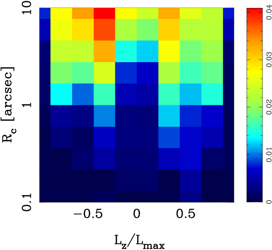
Figure 9: Reconstruction of the weighted two-integral DF of the lens galaxy SDSS J2321$-$097 obtained from the best-fitting model. Each pixel in the two-integral space gives the relative contribution of the corresponding TIC to the total mass of the modelled system. Here, $L_{\mathrm{max}}$ indicates the maximum value of the angular momentum along the $z$ axis: $L_{\mathrm{max}}=R_{\mathrm{c}}v_{\mathrm{c}}$, where $R_{\mathrm{c}}$ is the circular radius and $v_{\mathrm{c}}(R_{\mathrm{c}})$ is the circular velocity corresponding to a total energy $E(R_{\mathrm{c}})=\Phi_{\mathrm{eff}}(R_{\mathrm{c}},0)=\Phi(R_{\mathrm{c}},0)+v_{\mathrm{c}}^{2}/2$.

4.3 Inferences from the phase-space distribution

From the best reconstructed DF we calculate the axial ratio $q_{\mathrm{\star,3D}}$ of the three-dimensional light distribution, which does not need to coincide with the axial ratio of the total density distribution $\rho(m)$ since in our approach mass is not required to follow light. We adopt the definition

$$q_{\mathrm{\star,3D}}^{2}=2\frac{\int\rho_{\star}z^{2}\,\mathrm{d}V}{\int\rho_{\star}R^{2}\,\mathrm{d}V},$$ (8)

where $R$ and $z$ are the usual cylindrical coordinates and $V$ is the volume. This definition has been chosen such that a density distribution which is a function of the elliptical radius $\ell^{2}=R^{2}+z^{2}/{q_{\mathrm{ell}}}^{2}$ (e.g. a prolate or oblate ellipsoid of axial ratio $q_{\mathrm{ell}}$) gives $q_{\mathrm{\star,3D}}=q_{\mathrm{ell}}$. For our best model we obtain an axial ratio $q_{\mathrm{\star,3D}}=0.847$, which is rounder than the $q$ of the total density distribution. From the observed isophotal two-dimensional axial ratio $q_{\mathrm{iso,2D}}=0.77$ (measured by fitting ellipses to the surface brightness contours of the galaxy, Table 1) and from the best model inclination of $67\aas@@fstack{\circ}8$, one obtains a three-dimensional axial ratio of the stellar density of $q_{\mathrm{iso,3D}}=0.72$. This does not coincide with the value of $q_{\mathrm{\star,3D}}$ calculated from the second moments of the luminosity density of the galaxy (equation 8). The disagreement might indicate that the recovered three-dimensional light distribution is not constant on ellipsoidal surfaces or that there is a change in ellipticity as a function of radius.

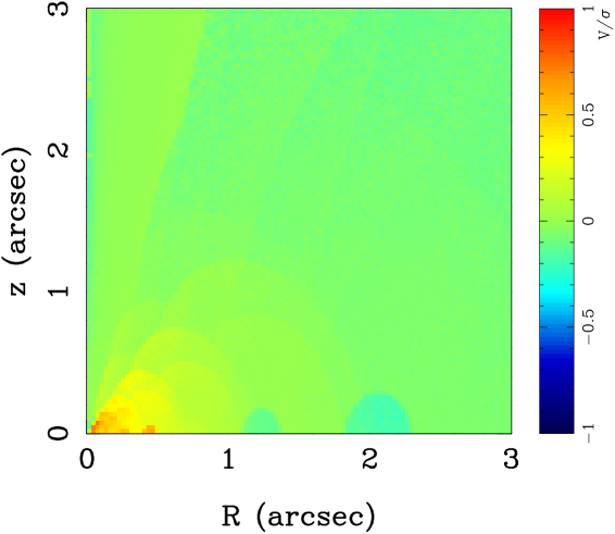
Figure 10: Ratio $\langle v_{\varphi}\rangle/\bar{\sigma}$ of the first and second velocity moments for the best reconstructed model of galaxy SDSS J2321$-$097, plotted in the positive quadrant of the meridional plane.

Following Cappellari et al. (2007), we plot in Fig. 10 the ratio $\langle v_{\varphi}\rangle/\bar{\sigma}$ in the meridional plane between the mean rotation velocity around the $z$-axis and the local mean velocity dispersion $\bar{\sigma}^{2}=(\sigma_{R}^{2}+\sigma_{\varphi}^{2}+\sigma_{z}^{2})/3$. This quantity provides an indication of the importance of the rotation with respect to the random motions for each position $(R,z)$ in the galaxy. From the analysis of Fig. 10, SDSS J2321$-$097 appears to be an overall slow rotator, although rotation seems to play a more significant role in the inner regions. Two small regions characterized by slight counter-rotation are located around the equatorial plane ($z\!=\!0$). Due to the assumption of a two-integral DF, the cross-section of the velocity dispersion ellipsoids would be circular for every position on the meridional plane.

Figure 11: Upper panel: mass enclosed within a radius $r$. The thick solid line shows the total mass of the galaxy as a function of $r$ obtained from the best reconstructed model. The thick dashed line shows the same quantity for the luminous component obtained from the reconstructed DF and rescaled to the value which maximizes the contribution of luminous over dark matter (‘maximum bulge’). As a comparison, the dash–dotted and dotted lines show the quantity $M(r)$ for, respectively, a Jaffe and a Hernquist profile, normalized to the total luminous mass. Lower panel: logarithm of circularized mass density as a function of radius. The line styles have the same meaning as above.

Another helpful way to quantify the anisotropy of an axisymmetric galaxy is provided by the three global anisotropy parameters defined in Binney & Tremaine (1987) and Cappellari et al. (2007):

$$\beta\equiv 1-\frac{\Pi_{zz}}{\Pi_{RR}},$$ (9)

$$\gamma\equiv 1-\frac{\Pi_{\varphi\varphi}}{\Pi_{RR}},$$ (10)

$$\delta\equiv 1-\frac{2\Pi_{zz}}{\Pi_{RR}+\Pi_{\varphi\varphi}}=\frac{2\beta-\gamma}{2-\gamma},$$ (11)

where

$$\Pi_{kk}=\int\rho\sigma^{2}_{k}\,\mathrm{d}^{3}x$$ (12)

and $\sigma_{k}$ denotes the velocity dispersion along the direction $k$ at any given location in the galaxy. For nearly spherical systems it can be convenient to consider the anisotropy parameter $\beta_{r}$ defined as

$$\beta_{r}\equiv 1-\frac{\Pi_{tt}}{\Pi_{rr}}$$ (13)

in the spherical coordinates $(r,\theta,\varphi)$. Here $\Pi_{tt}=(\Pi_{\theta\theta}+\Pi_{\varphi\varphi})/2$.

For a two-integral DF, as mentioned above, $\sigma_{R}^{2}=\sigma_{z}^{2}$ everywhere, which implies $\Pi_{RR}=\Pi_{zz}$. Therefore, the value of $\beta$ is always zero, while $\gamma$ and $\delta$ have opposite signs. Moreover, under this assumption it is easy to show that $\beta_{r}=\gamma/2$.

Calculating the non-zero anisotropy parameters for the best reconstructed model, we find $\gamma=-0.32$, which indicates a slight tangential anisotropy, and $\delta=0.14$. The latter value agrees well with the corresponding value determined directly from the observed data in Section 3.3. The anisotropy parameters found for SDSS J2321$-$097 have values which are consistent with the findings of Cappellari et al. (2007) for their most luminous galaxies. It should be pointed out, however, that the comparison is not immediately straightforward, since their use of a three-integral Schwarzschild orbit-superposition method gives more flexibility to the models.

We compared the radial profile of the total mass density of the galaxy (given by equation 3 by inserting the best-fitting model parameters) with the density of the stellar component alone, as obtained directly from the reconstructed DF. The axisymmetric density distribution was circularized by averaging over spherical shells. The stellar density profile has been normalized by using as a constraint the value $M_{\mathrm{eff}}\simeq 2.0\times 10^{11}M_{\sun}$ for the luminous mass inside the effective radius, which is obtained from the observations when assuming an average $M/L$ of $5.2~{}(M/L)_{\sun,B}$. This ‘maximum bulge’ rescaling (analogous to the maximum disc approach for spiral galaxies) maximizes the contribution of the luminous component with respect to the total mass. The density and the enclosed mass as a function of radius are plotted in Fig. 11, together with the same functions for the spherical Jaffe and Hernquist profiles (Jaffe, 1983; Hernquist, 1990) normalized to the total mass $2M_{\mathrm{eff}}$. While very simple, these models appear to provide a reasonably good approximation to the light distribution. From the diagrams, one can note that the total mass density distribution follows the light in the inner regions up to a distance of about 5 kpc, where the contribution of the dark matter component starts to become significant: at 5 kpc the non-visible mass represents about 15 per cent of the total mass, rising to $\sim 30$ per cent at 10 kpc (the distance for which the enclosed stellar mass approximately equals $M_{\mathrm{eff}}$, i.e. the distance corresponding to the unprojected effective radius) and $\sim 40$ per cent at 15 kpc.

The spatial coverage of the data might appear quite limited when it comes to the study of the total density profile at radii of the order of 10 kpc, since the Einstein radius $R_{\mathrm{Einst}}\simeq 2.6\,\mathrm{kpc}$, the effective radius $R_{\mathrm{eff}}$ is of the order of 8 kpc (which however becomes $\sim 10$ kpc when unprojected) and the integral-field kinematics does not extend much farther than 3 kpc. However, one should note that a fair amount of information comes also from those distant regions of the galaxy that are seen in projection along the line of sight. In order to verify this, we consider the intersection between a sphere of radius $r$, centred on the galaxy, and a cylinder oriented along the line of sight which has a radius equal to, respectively, the Einstein radius and the effective radius. In the first case, it is found that for $r=R_{\mathrm{Einst}}$ the mass enclosed within this volume corresponds to approximately 75 per cent of $M_{\mathrm{Einst}}$ (the total mass within the Einstein radius). In other words, one-fourth of the contribution to the gravitational lensing comes from matter which is located farther than 2.6 kpc but falls, in projection, within the Einstein radius. In the second case, we obtain that for $r=R_{\mathrm{eff}}$ the enclosed light is about 77 per cent of $L_{\mathrm{eff}}$, that is, again almost one-fourth of the luminosity enclosed within the cylinder of radius $R_{\mathrm{eff}}$ comes from regions at a radial distance $r>R_{\mathrm{eff}}$ from the centre of the galaxy. Any changes in the density distribution at radial distances larger than $R_{\mathrm{Einst}}$ or $R_{\mathrm{eff}}$ which still influence the data model inside those projected radii will have an effect which is reflected statistically in the evidence (or in the likelihood), allowing to discriminate between different models. Clearly, the effect becomes progressively weaker with increasing radial distances.

We also explored a constant-$M/L$ model, by considering a double power-law density distribution which approximates the reconstructed luminous density profile of Fig. 11: this density profile is nearly isothermal in the inner regions but the slope becomes significantly steeper ($\gamma^{\prime}_{\mathrm{out}}\sim 3.3$) outwards. The $M/L$ is $5.9\,(M/L)_{\sun,B}$. We find that the constant-$M/L$ model, while able to reproduce the data, fits the dynamics somewhat worse: the $\chi^{2}$ per pixel for the velocity dispersion is $\sim 2.2$, higher than in the case of the single power-law model ($\chi^{2}$ per pixel $\sim 1.4$). For the lensing and the surface brightness distribution, instead, the values of $\chi^{2}$ per pixel of the two models are comparable (with the double power law being just a few per cent higher). In conclusion, under the considered assumptions, the nearly isothermal single power-law model is slightly preferred by the data over a constant-$M/L$ model with no dark matter. It should be noted, however, that the difference between the constant-$M/L$ model and the power-law model (for which mass does not need to follow light) is relatively small. It is possible that much or all of this discrepancy could disappear if one allowed for more sophisticated three-integral dynamical models.

4.4 Uncertainties

Table 3: Summary of the model uncertainties, determined by considering 128 random realizations of the best model data sets. The reconstructed parameters obtained for the best model $\mathcal{M}_{\mathrm{best}}$ are also reported for comparison.

		Median	Mean	68 per cent confidence interval	95 per cent confidence interval	$\mathcal{M}_{\mathrm{best}}$
	$i$	$66\aas@@fstack{\circ}1$	$65\aas@@fstack{\circ}2$	[$60\aas@@fstack{\circ}0$, $68\aas@@fstack{\circ}9$]	[$55\aas@@fstack{\circ}1$, $75\aas@@fstack{\circ}8$]	$67\aas@@fstack{\circ}8$
Non-linear	$\alpha_{0}$	0.472	0.472	[0.467, 0.475]	[0.463, 0.479]	0.468
parameters	$\gamma^{\prime}$	2.061	2.046	[1.996, 2.085]	[1.894, 2.142]	2.061
	$q$	0.739	0.730	[0.688, 0.760]	[0.657, 0.802]	0.739

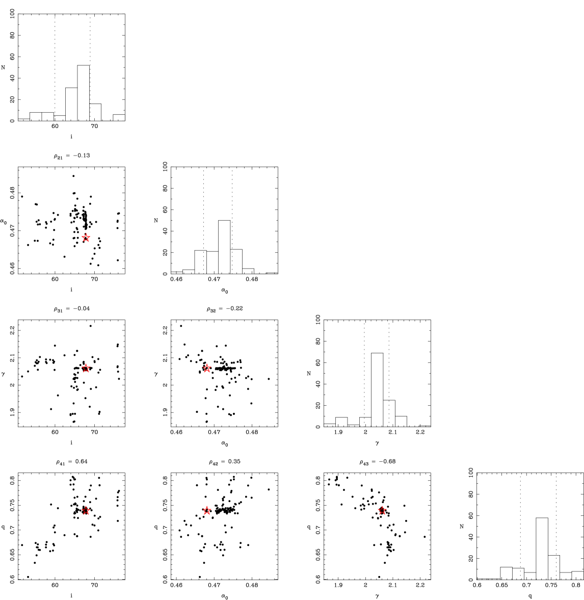
Figure 12: Graphical visualization of the lower triangle of the (symmetric) correlation matrix for the parameters recovered from the non-linear reconstruction of 128 random realizations of the best model data sets. The panels on the main diagonal present the distribution of the four non-linear parameters $i$, $\alpha_{0}$, $\gamma^{\prime}$ and $q$ over the realizations. In the remaining panels the non-linear parameters are plotted two by two against each other; for each panel, the corresponding value $\rho_{ij}$ of the correlation matrix is also indicated. The dotted vertical lines indicate the 68 per cent confidence interval. The red stars indicate the locations of the parameters obtained from the best model reconstruction $\mathcal{M}_{\mathrm{best}}$ (cf. Table 2).

The model uncertainties, that is, the scatter in the recovered non-linear parameters $i$, $\alpha_{0}$, $\gamma^{\prime}$ and $q$, were determined by considering 128 random realizations of the datasets and rerunning the cauldron algorithm for each of them. Table 3 summarizes the results of the statistical analysis and shows the 68 and 95 per cent confidence intervals for the four non-linear parameters. Fig. 12 shows a graphical visualization of the correlation matrix, displaying the parameters plotted against each other, while the histograms on the main diagonal present the distribution of the four parameters over the realizations. These distributions, which provide the error bars for the best-fitting model parameters, can immediately be seen to be generally non-Gaussian.

As highlighted in BK07, there appears to be a partial degeneracy between the inclination $i$ and the axial ratio $q$, which is however limited only within a certain interval in the parameters. The lens strength $\alpha_{0}$ is quite tightly constrained, and the logarithmic slope $\gamma^{\prime}$ spans over an interval of values all very close to the isothermal $\gamma^{\prime}=2$ case.

5 Breaking degeneracies: oblateness and inclination

When combining stellar kinematic and gravitational lensing data of an early-type galaxy, even under the simplifying assumption of spherical symmetry, it has been shown that the degeneracies between mass, orbital anisotropy and total density slope can effectively be broken (e.g. Treu & Koopmans, 2002a; Koopmans et al., 2003; Koopmans & Treu, 2003; Treu & Koopmans, 2004; Koopmans et al., 2006). More recently, the theoretical basis of this methodology was made self-consistent and extended to include flattened axisymmetric mass distributions and the modelling of the stellar two-integral phase-space DF $f(E,L_{z})$ (BK07). It was shown that under the assumptions of axisymmetry and two-integral DFs not only the degeneracy between mass, mass slope and anisotropy can be broken, but also that between the flattening (i.e. oblateness) of the mass distribution and its inclination with respect to an observer. The latter degeneracy poses a restriction on most current dynamical modelling efforts, which often have to assume some (range of) inclination (e.g. Emsellem et al., 2007; Cappellari et al., 2007).

By combining the information from lensing and dynamics we have found a well-defined mass slope (consistent with Koopmans et al. 2006), inclination and oblateness for the early-type lens galaxy SDSS J2321$-$097 (see e.g. Fig. 12). In this section, we show why the degeneracy between oblateness and inclination can, in principle, be broken. As in all of this paper, we assume axisymmetry and restrict the phase-space density distribution to be a function of the two classical integrals of motion, $E$ and $L_{z}$ (these assumptions hold well in the system considered in this paper). In this case, it can be shown from symmetry arguments (Binney & Tremaine, 1987) that at any point in the galaxy the two-dimensional cut through the stellar velocity ellipsoid in the meridional plane $(R,z)$ is round (i.e. $\sigma_{R}=\sigma_{z}$). For an observer located in the meridional plane, the line-of-sight component of the stellar velocity dispersion from any given point on the same plane will therefore appear independent of inclination. The luminosity-weighted integral of the stellar velocity dispersion over the entire meridional plane is then also independent of inclination. Because an observer is always situated in the meridional plane spanned by himself and the minor axis of an axisymmetric galaxy, we state that:

The surface brightness weighted integral over the line-of-sight stellar velocity dispersion along the minor axis of an axisymmetric galaxy with a DF that depends only on energy and angular momentum, $f(E,L_{z})$, is independent of inclination. This also holds in the case of streaming motions which are perpendicular to the minor axis.

This can be formally proved as follows. The luminosity-weighted stellar velocity dispersion integrated over the meridional plane of a galaxy with inclination $i=0$ is given by

$$\langle\sigma_{\mathrm{mp}}^{2}\rangle(i=0)=\frac{\int_{-\infty}^{\infty}\int_{-\infty}^{\infty}\sigma^{2}_{\mathrm{los}}(R,z)\,\rho_{\star}(R,z)\,\mathrm{d}R\,\mathrm{d}z}{\int_{-\infty}^{\infty}\int_{-\infty}^{\infty}\rho_{\star}(R,z)\,\mathrm{d}R\,\mathrm{d}z}\,.$$ (14)

Under a rotation, denoted by the orthogonal rotational matrix $\mathbf{R}(i)$ with $\det\mathbf{R}(i)=\det\mathbf{R}^{-1}(i)=1$, the coordinate system can be transformed as $\mn@boldsymbol{x}^{\prime}=\mathbf{R}(i)\mn@boldsymbol{x}$ with $\mn@boldsymbol{x}\equiv(R,z)$ and $\mn@boldsymbol{x}^{\prime}\equiv(R^{\prime},z^{\prime})$. The above equation can then, after coordinate transformation, be written as

$$\langle\sigma_{\mathrm{mp}}^{2}\rangle(i)=\frac{\int_{-\infty}^{\infty}\int_{-\infty}^{\infty}\sigma^{2}_{\mathrm{los}}(R^{\prime},z^{\prime})\,\rho_{\star}(R^{\prime},z^{\prime})\,\det\mathbf{R}^{-1}(i)\,\mathrm{d}R^{\prime}\,\mathrm{d}z^{\prime}}{\int_{-\infty}^{\infty}\int_{-\infty}^{\infty}\rho_{\star}(R^{\prime},z^{\prime})\,\det\mathbf{R}^{-1}(i)\,\mathrm{d}R^{\prime}\,\mathrm{d}z^{\prime}}.$$ (15)

Because rotation does not alter the line-of-sight velocity dispersion of a given point in the meridional plane if the potential is axisymmetric and the DF is only a function of $E$ and $L_{z}$, it is easy to see that $\sigma^{2}_{\mathrm{los}}(R^{\prime},z^{\prime})=\sigma^{2}_{\mathrm{los}}(R,z)$ for any inclination $i$. Also the scalar $\rho_{\star}$ is invariant under rotation, hence $\rho_{\star}(R^{\prime},z^{\prime})=\rho_{\star}(R,z)$. Given the fact that $\det\mathbf{R}^{-1}(i)=1$, it immediately follows that

$$\langle\sigma_{\mathrm{mp}}^{2}\rangle(i)\equiv\langle\sigma_{\mathrm{mp}}^{2}\rangle(i=0),$$ (16)

proving the above statement. Hence, $\langle\sigma_{\mathrm{mp}}^{2}\rangle(i)$ effectively becomes a function only of the density profile, mass and flattening of the mass distribution. Since the former two are well constrained by gravitational lensing alone and even better in combination with the stellar kinematics, $\langle\sigma_{\mathrm{mp}}^{2}\rangle(i)$ reduces further to a function of mostly the oblateness: for a given mass and mass profile, a more oblate galaxy will have a larger value of $\langle\sigma_{\mathrm{mp}}^{2}\rangle(i)$. Because $q_{\mathrm{\star,3D}}$ and inclination are restricted by the observed brightness distribution of the galaxy, and the oblateness by the value of $\langle\sigma_{\mathrm{mp}}^{2}\rangle$, one can solve for the inclination and oblateness simultaneously.

From the IFU data the value of $\langle\sigma_{\mathrm{mp}}^{2}\rangle$ can be inferred (because of the limited field of view, we cannot integrate over the entire minor axis and $\langle\sigma_{\mathrm{mp}}^{2}\rangle$ might therefore still be a weak function of $i$) and in combination with the observed flattening of the galaxy brightness distribution, the inclination can be inferred. It is clear that this can only be done when the stellar velocity dispersion along the entire minor axis is known and that the inclination cannot be inferred from a total luminosity-weighted stellar velocity dispersion.

We again emphasize here that the above result only holds in axisymmetric two-integral situations. To what extent it remains valid in cases where a third integral of motion is allowed (or axisymmetry is broken), remains a subject of further study.

6 Discussion and conclusions

In this paper we have presented the first results from an integral-field spectroscopic survey of early-type lens galaxies from SLACS. The combination of integral-field spectroscopy from VIMOS/IFU mounted on the VLT with high-resolution imaging from HST/ACS has enabled us to conduct the first in-depth study of the structure of a luminous elliptical galaxy beyond the local Universe, SDSS J2321$-$097 at $z=0.0819$. We have applied a new analysis method that combines the kinematic and lensing information in a fully self-consistent way and have shown how this combination breaks some of the degeneracies that limit the separate application of these two methods.

The galaxy that we have studied here turns out to be a fairly ordinary elliptical with properties similar to those of local galaxies of comparable luminosity, such as those studied by the SAURON collaboration (Emsellem et al., 2007; Cappellari et al., 2007). SDSS J2321$-$097 is a slow rotator in the classification of Emsellem et al. (2007) with an angular momentum parameter of $\lambda_{\mathrm{R}}=0.075$. The velocity dispersion map is flat to the limit where we were able to measure the kinematic parameters reliably. Using the updated estimator of Binney (2005) for the ratio between systematic and random velocities, $v/\sigma_{v}$, that fully exploits the information in integral-field spectroscopic data, we have shown that the ellipticity of the stellar distribution in SDSS J2321$-$097 is due to anisotropy of the velocity distribution rather than rotation, again in line with local galaxies of comparable luminosity (Cappellari et al., 2007).

We have modelled the galaxy by making use of the cauldron algorithm which self-consistently combines gravitational lensing and stellar dynamics under the assumption of axisymmetry and a two-integral DF. We adopted for the system the total gravitational potential generated by an axisymmetric power-law mass density distribution of logarithmic slope $\gamma^{\prime}$ and axial ratio $q$. The best-fitting model given the data is obtained in the framework of Bayesian statistics by maximizing the evidence merit function. The results for the best-fitting model are summarized as follows.

1. The logarithmic slope of the total density is $\gamma^{\prime}=2.06^{+0.03}_{-0.06}$ (the error is given within the 68 per cent confidence interval), which is very close to (and consistent with) an isothermal density distribution.

2. The axial ratio of the total density distribution is $q=0.74^{+0.02}_{-0.05}$. Since in our approach mass is not required to follow light, this $q$ does not have to coincide with the (average) axial ratio of the luminous distribution, which is calculated from the reconstructed DF, giving $q_{\mathrm{\star,3D}}=0.85$ for the best model.

3. The inclination angle of the galaxy is $i=67\aas@@fstack{\circ}8^{+1.1}_{-7.8}$. The small error bar shows that inclination can be well determined in combination with lensing data.

4. The ‘maximum bulge’ approach, that is, the rescaling of the circularized stellar density profile which maximizes the contribution of the luminous component to the total density profile, prescribes a stellar mass $M_{\mathrm{eff}}\simeq 2.0\times 10^{11}M_{\sun}$ inside the effective radius, which corresponds to an average $M/L$ of $5.2\,(M/L)_{\sun,B}$. The total mass enclosed in the same region is approximately $2.9\times 10^{11}M_{\sun}$: the non-visible matter, therefore, accounts for about 30 per cent of the total mass within that three-dimensional radius.

5. The local $\langle v_{\varphi}\rangle/\bar{\sigma}$ ratio on the meridional plane confirms that SDSS J2321$-$097 as a whole is a slow rotator, with the random motions becoming less predominant compared to rotation only in the very central regions. The best model yields a global anisotropy parameter $\delta=0.14$, fully consistent with the value obtained directly from the data, showing that the galaxy is close to an isotropic rotator. The other global anisotropy parameters have values $\beta=0$ [as a consequence of having assumed a two-integral DF $f(E,L_{z})$] and $\gamma=-0.32$, indicating a mild tangential anisotropy.

These results are in good agreement with the analysis of SDSS J2321$-$097 by Koopmans et al. (2006), which we here extend in a more rigorous way. In particular, the results confirm the essentially isothermal profile of the mass density distribution, which appears to be a defining characteristic of early-type galaxies.

The best-fitting model is consistent with a dark matter fraction of 30 per cent within 10 kpc (approximately corresponding to the unprojected effective radius), similar to what Cappellari et al. (2006) determine for the SAURON sample of early-type galaxies by making use of three-integral Schwarzschild dynamical models under the caveat that light traces mass. However, it seems plausible that a constant-M/L model could still reproduce the observed kinematics of SDSS J2321$-$097 if one allowed for a more flexible three-integral dynamical model rather than the two-integral model considered in this work. The relative difficulty in unambiguously discriminating between the constant-$M/L$ model and the power-law model is also a consequence of the fact that for the specific lens system studied here, the mass within the Einstein radius is to a large extent dominated by the stellar mass, so that the difference between the two models does not show up dramatically in the lens model. The combined analysis of more distant objects, however, is expected to provide more unequivocal results in this respect. In general, for galaxies at higher redshift the ratio between the Einstein radius and the effective radius becomes larger (see e.g. the SLACS galaxy sample in Koopmans et al. 2006) and any deviation from a model for which mass follows light would become significantly more prominent, since at least the surface brightness slope would be much steeper than what is allowed by the lensing data.

The dynamical structure of SDSS J2321$-$097 (i.e. anisotropy and $\langle v_{\varphi}\rangle/\bar{\sigma}$ map) is also in good agreement with what is found by Cappellari et al. (2007) for the most massive ellipticals of the SAURON sample.

The analysis has shown that the combination of gravitational lensing and stellar dynamics is a powerful method which allows the dissection in three dimensions of an elliptical galaxy (assumed to be well described as a two-integral axisymmetric dynamical system), breaking to a significant extent the classical degeneracies between inclination and flattening as well as between mass and anisotropy. The way the degeneracy between inclination and oblateness is overcome can be understood within a simplified physical picture: $q$ and $i$ are coupled in the projected potential which enters in the description of gravitational lensing; when it comes to the dynamics, however, the surface brightness weighted integral along the minor axis over the line-of-sight stellar velocity dispersion is not a function of the inclination, since, due to the properties of the two-integral DF, the intersection of the velocity dispersion tensor with the $(v_{R},v_{z})$ plane is always a circle, that is, $\sigma_{R}^{2}=\sigma_{z}^{2}$ for each position in the galaxy (see Section 5).

We have shown that the method, in its implementation as the cauldron algorithm, is robust enough to make use of observational data in order to recover the non-linear parameters which characterize the total gravitational potential and the geometry of the system (i.e. inclination, positional angle and lens centre) with relatively tight error bars (the confidence intervals shown in Table 3). This first application therefore shows promise for the future study of the other SLACS systems at higher redshift.

In forthcoming papers in this series we will extend this work to the entire sample of 17 SLACS lenses with VLT VIMOS IFS, covering a range of lens galaxy morphology, mass and redshift ($z=0.08-0.35$). The VLT sample will be complemented by a further 13 lenses for which we have obtained long-slit spectroscopy at the Low Resolution Imager and Spectrograph (LRIS, Oke et al., 1995) on the Keck-I telescope. Several slit positions – aligned with the major axis and offset along the minor axis – have been obtained for each system in the Keck sample, thus effectively producing two-dimensional kinematic information across most of the lens galaxy.

References

- Arnaboldi et al. (1996) Arnaboldi, M. et al. 1996, ApJ, 472, 145
- Barnabè & Koopmans (2007) Barnabè, M., & Koopmans, L. V. E. 2007, ApJ, 666, 726
- Barth et al. (2002) Barth, A. J., Ho, L. C., & Sargent, W. L. W. 2002, AJ, 124, 2607
- Bertin et al. (1994) Bertin, G. et al. 1994, A&A, 292, 381
- Binney (2005) Binney, J. 2005, MNRAS, 363, 937
- Binney & Tremaine (1987) Binney, J., & Tremaine, S. 1987, Galactic dynamics (Princeton, NJ, Princeton University Press, 1987, 747 p.)
- Bolton & Burles (2007) Bolton, A. S., & Burles, S. 2007, New Journal of Physics, 9, 443
- Bolton et al. (2005) Bolton, A. S., Burles, S., Koopmans, L. V. E., Treu, T., & Moustakas, L. A. 2005, ApJ, 624, L21
- Bolton et al. (2006) —. 2006, ApJ, 638, 703
- Bolton et al. (2004) Bolton, A. S., Burles, S., Schlegel, D. J., Eisenstein, D. J., & Brinkmann, J. 2004, AJ, 127, 1860
- Bolton et al. (2007) Bolton, A. S., Burles, S., Treu, T., Koopmans, L. V. E., & Moustakas, L. A. 2007, ApJ, 665, L105
- Borriello et al. (2003) Borriello, A., Salucci, P., & Danese, L. 2003, MNRAS, 341, 1109
- Browne et al. (2003) Browne, I. W. A. et al. 2003, MNRAS, 341, 13
- Burkert & Naab (2004) Burkert, A., & Naab, T. 2004, in Coevolution of Black Holes and Galaxies, from the Carnegie Observatories Centennial Symposia, ed. L. C. Ho, Carnegie Observatories Astrophysics Series (Cambridge University Press), 421
- Cappellari et al. (2006) Cappellari, M. et al. 2006, MNRAS, 366, 1126
- Cappellari & Emsellem (2004) Cappellari, M., & Emsellem, E. 2004, PASP, 116, 138
- Cappellari et al. (2007) Cappellari, M. et al. 2007, MNRAS, 379, 418
- Carollo et al. (1995) Carollo, C. M., de Zeeuw, P. T., van der Marel, R. P., Danziger, I. J., & Qian, E. E. 1995, ApJ, 441, L25
- Chandrasekhar (1969) Chandrasekhar, S. 1969, Ellipsoidal Figures of Equilibrium (New Haven: Yale University Press)
- Ciotti & Bertin (2005) Ciotti, L., & Bertin, G. 2005, A&A, 437, 419
- Cretton et al. (1999) Cretton, N., de Zeeuw, P. T., van der Marel, R. P., & Rix, H.-W. 1999, ApJS, 124, 383
- de Bruyne et al. (2003) de Bruyne, V., Vauterin, P., de Rijcke, S., & Dejonghe, H. 2003, MNRAS, 339, 215
- de Zeeuw et al. (2002) de Zeeuw, P. T. et al. 2002, MNRAS, 329, 513
- Djorgovski & Davis (1987) Djorgovski, S., & Davis, M. 1987, ApJ, 313, 59
- Dressler et al. (1987) Dressler, A., Lynden-Bell, D., Burstein, D., Davies, R. L., Faber, S. M., Terlevich, R., & Wegner, G. 1987, ApJ, 313, 42
- Eisenstein et al. (2001) Eisenstein, D. J. et al. 2001, AJ, 122, 2267
- Emsellem et al. (2007) Emsellem, E. et al. 2007, MNRAS, 379, 401
- Emsellem et al. (2004) —. 2004, MNRAS, 352, 721
- Fabbiano (1989) Fabbiano, G. 1989, ARAA, 27, 87
- Franx et al. (1994) Franx, M., van Gorkom, J. H., & de Zeeuw, P. T. 1994, ApJ, 436, 642
- Gavazzi et al. (2007) Gavazzi, R., Treu, T., Rhodes, J. D., Koopmans, L. V. E., Bolton, A. S., Burles, S., Massey, R. J., & Moustakas, L. A. 2007, ApJ, 667, 176
- Gerhard et al. (2001) Gerhard, O., Kronawitter, A., Saglia, R. P., & Bender, R. 2001, AJ, 121, 1936
- Hernquist (1990) Hernquist, L. 1990, ApJ, 356, 359
- Horne (1986) Horne, K. 1986, PASP, 98, 609
- Jaffe (1983) Jaffe, W. 1983, MNRAS, 202, 995
- Koopmans et al. (2006) Koopmans, L., Treu, T., Bolton, A. S., Burles, S., & Moustakas, L. A. 2006, ApJ, 649, 599
- Koopmans & Treu (2002) Koopmans, L. V. E., & Treu, T. 2002, ApJ, 568, L5
- Koopmans & Treu (2003) —. 2003, ApJ, 583, 606
- Koopmans et al. (2003) Koopmans, L. V. E., Treu, T., Fassnacht, C. D., Blandford, R. D., & Surpi, G. 2003, ApJ, 599, 70
- Krist (1993) Krist, J. 1993, in ASP Conf. Ser., Vol. 52, Astronomical Data Analysis Software and Systems II, ed. R. J. Hanisch, R. J. V. Brissenden, & J. Barnes (San Francisco: Astron. Soc. Pac.), 536
- Le Fèvre et al. (2001) Le Fèvre, O. et al. 2001, in Deep Fields: Proceedings of the ESO/ECF/STScI Workshop held at Garching, Germany, 9-12 October 2000, ed. S. Cristiani, A. Renzini, & R. E. Williams (Berlin/Heidelberg: Springer-Verlag), 236
- Loewenstein & White (1999) Loewenstein, M., & White, R. E. 1999, ApJ, 518, 50
- MacKay (1992) MacKay, D. J. C. 1992, PhD thesis, California Institute of Technology
- MacKay (1999) —. 1999, Neural Comp, 11, 1035
- MacKay (2003) —. 2003, Information Theory, Inference and Learning Algorithms (Cambridge: Cambridge University Press)
- Magorrian et al. (1998) Magorrian, J. et al. 1998, AJ, 115, 2285
- Matsushita et al. (1998) Matsushita, K., Makishima, K., Ikebe, Y., Rokutanda, E., Yamasaki, N., & Ohashi, T. 1998, ApJ, 499, L13
- Merritt & Fridman (1996) Merritt, D., & Fridman, T. 1996, ApJ, 460, 136
- Mould et al. (1990) Mould, J. R., Oke, J. B., de Zeeuw, P. T., & Nemec, J. M. 1990, AJ, 99, 1823
- Oke et al. (1995) Oke, J. B. et al. 1995, PASP, 107, 375
- R Development Core Team (2007) R Development Core Team. 2007, R: A Language and Environment for Statistical Computing, R Foundation for Statistical Computing, Vienna, Austria, ISBN 3-900051-07-0
- Rix et al. (1997) Rix, H., de Zeeuw, P. T., Cretton, N., van der Marel, R. P., & Carollo, C. M. 1997, ApJ, 488, 702
- Romanowsky et al. (2003) Romanowsky, A. J., Douglas, N. G., Arnaboldi, M., Kuijken, K., Merrifield, M. R., Napolitano, N. R., Capaccioli, M., & Freeman, K. C. 2003, Science, 301, 1696
- Saglia et al. (1992) Saglia, R. P., Bertin, G., & Stiavelli, M. 1992, ApJ, 384, 433
- Schwarzschild (1979) Schwarzschild, M. 1979, ApJ, 232, 236
- Scodeggio et al. (2005) Scodeggio, M. et al. 2005, PASP, 117, 1284
- Seljak (2002) Seljak, U. 2002, MNRAS, 334, 797
- Strauss et al. (2002) Strauss, M. A. et al. 2002, AJ, 124, 1810
- Suyu et al. (2006) Suyu, S. H., Marshall, P. J., Hobson, M. P., & Blandford, R. D. 2006, MNRAS, 371, 983
- Treu & Koopmans (2002a) Treu, T., & Koopmans, L. V. E. 2002a, ApJ, 575, 87
- Treu & Koopmans (2002b) —. 2002b, MNRAS, 337, L6
- Treu & Koopmans (2003) —. 2003, MNRAS, 343, L29
- Treu & Koopmans (2004) —. 2004, ApJ, 611, 739
- Treu et al. (2006a) Treu, T., Koopmans, L. V. E., Bolton, A. S., Burles, S., & Moustakas, L. 2006a, ApJ, 650, 1219
- Treu et al. (2006b) —. 2006b, ApJ, 640, 662
- Turner et al. (1984) Turner, E. L., Ostriker, J. P., & Gott, III, J. R. 1984, ApJ, 284, 1
- Valdes et al. (2004) Valdes, F., Gupta, R., Rose, J. A., Singh, H. P., & Bell, D. J. 2004, ApJS, 152, 251
- van der Marel (1994) van der Marel, R. P. 1994, MNRAS, 270, 271
- van der Marel & Franx (1993) van der Marel, R. P., & Franx, M. 1993, ApJ, 407, 525
- Verolme & de Zeeuw (2002) Verolme, E. K., & de Zeeuw, P. T. 2002, MNRAS, 331, 959
- Zanichelli et al. (2005) Zanichelli, A. et al. 2005, PASP, 117, 1271