Synchronization of phase oscillators with heterogeneous coupling: A solvable case

Abstract

We consider an extension of Kuramoto’s model of coupled phase oscillators where oscillator pairs interact with different strengths. When the coupling coefficient of each pair can be separated into two different factors, each one associated to an oscillator, Kuramoto’s theory for the transition to synchronization can be explicitly generalized, and the effects of coupling heterogeneity on synchronized states can be analytically studied. The two factors are respectively interpreted as the weight of the contribution of each oscillator to the mean field, and the coupling of each oscillator to that field. We explicitly analyze the effects of correlations between those weights and couplings, and show that synchronization can be completely inhibited when they are strongly anti-correlated. Numerical results validate the theory, but suggest that finite-size effect are relevant to the collective dynamics close to the synchronization transition, where oscillators become entrained in synchronized frequency clusters.

and

1 Introduction

Macroscopic periodic oscillations are ubiquitous in living organisms, and span a broad range of time scales, from fractions of a second –such as in neural and heart tissues– to days or weeks –such as in circadian rhythms and menstrual cycles. The possibility that this kind of macroscopic dynamics is the collective manifestation of mutual synchronization of microscopic oscillations was advanced by N. Wiener in the 1940s [1], and was later elaborated by A. T. Winfree [2, 3]. The basic mechanism assumed to be at work in this self-organization phenomenon is that a few elements in a population of interacting oscillators may synchronize if they have similar frequencies and their coupling is strong enough. Under suitable conditions, other oscillators may in turn be entrained by this “nucleation center” and, eventually, contribute to form a macroscopic oscillating cluster. Collective oscillations would thus emerge as the result of coherent microscopic dynamics, through a process not unlike a condensation phase transition [2].

This conceptual idea was realized into an explicit model by Y. Kuramoto [4], who considered the collective dynamics of an ensemble of $N$ globally coupled phase oscillators. The state of each oscillator is defined by its phase $\phi_{i}(t)\in[0,2\pi)$. Their joint evolution is governed by the equations

$$\dot{\phi}_{i}=\omega_{i}+\frac{K}{N}\sum_{j=1}^{N}\sin(\phi_{j}-\phi_{i}),$$ (1)

($i=1,\dots,N$) where $\omega_{i}$ is the natural frequency of oscillator $i$, and $K$ is the strength of their global (all-to-all) coupling. In this system, synchronized states can be characterized by the distribution of effective frequencies $\omega_{i}^{\prime}$. The effective frequency of an oscillator is defined as the time average of its phase velocity:

$$\omega_{i}^{\prime}=\lim_{T\to\infty}\frac{1}{T}\int_{0}^{T}\dot{\phi}_{i}dt.$$ (2)

It is found that, for sufficiently large $K$, there is a group of oscillators whose effective frequencies are identical. The number of these synchronized oscillators increases with $K$. Synchronization implies as well a certain degree of order in the distribution of the individual oscillator phases. This is revealed by the complex order parameter

$$z(t)\equiv\sigma(t)\exp[{\rm i}\Phi(t)]=\frac{1}{N}\sum_{j=1}^{N}\exp\left[{\rm i}\phi_{j}(t)\right].$$ (3)

Kuramoto showed that in the limit $N\to\infty$, and under the assumption that synchronized oscillators form a single group with effective frequency $\omega_{i}^{\prime}=\Omega$, the collective amplitude $\sigma$ –which turns out to be independent of time– vanishes for coupling intensities below a certain critical value $K_{c}$, and is different from zero for $K>K_{c}$ [4]. The threshold $K_{c}$ of the synchronization transition is determined by the distribution of natural frequencies $\omega_{i}$: ensembles with wider frequency distributions require stronger coupling to become synchronized. As a byproduct of the formulation, the synchronization frequency $\Omega$ is also obtained, and $\Phi(t)=\Phi(0)+\Omega t$.

The quantity $z(t)$ can be interpreted as a mean field generated by the oscillator ensemble. In fact, $\sigma(t)$ and $\Phi(t)$ define, respectively, the collective amplitude and phase of the ensemble. The evolution equation (1) for each oscillator can be rewritten as

$$\dot{\phi}_{i}=\omega_{i}+K\sigma\sin(\Phi-\phi_{i}).$$ (4)

The coupling of oscillator $i$ with the ensemble is thus represented as the interaction with a single, equivalent oscillator of phase $\Phi$, weighted by the amplitude $\sigma$.

The synchronization transition results from the competing effect of two factors: while coupling induces the emergence of ordered dynamics, the heterogeneity in the distribution of natural frequencies favours incoherent behaviour [5]. The aim of the present paper is to incorporate two additional sources of heterogeneity to Kuramoto’s model. First, we consider that each oscillator $i$ is coupled to the mean field $z=\sigma\exp({\rm i}\Phi)$ with its own coupling intensity $k_{i}$. Second, we assume that the individual contribution of each oscillator to the mean field is weighted by a factor $q_{i}$. In contrast with natural frequencies, which determine the individual dynamics in the absence of coupling, the two new attributes $k_{i}$ and $q_{i}$ affect the way in which each oscillator interacts with the ensemble. Therefore, they define a heterogeneous interaction pattern underlying the system.

Heterogeneity is a widespread feature in multi-agent systems. Constitutional differences between the members of such systems imply variations in the individual dynamics, in the response to external influxes, in the interaction with other elements, etc. Those differences may also have non-trivial effects on the collective dynamics of the ensemble [3, 6]. In connection with a more realistic representation of both natural and artificial systems, it is therefore desirable to generalize standard models in order to encompass heterogeneity. The present extension of the phase-oscillator model has the additional interest of being analytically tractable through a rather straightforward generalization of Kuramoto’s theory. In fact, in the limit of an infinitely large ensemble, the synchronization transition, as well as the collective dynamical properties of the synchronized state, can be fully characterized in the frame of such generalization.

In the next section, we discuss how Kuramoto’s theory is extended to include the form of heterogeneous coupling advanced above. We establish self-consistency equations for the collective amplitude and the synchronization frequency, and find the frequency distribution of non-synchronized oscillators. In Section 3, the results of Section 2 are applied to analyze synchronization properties in several specific cases, paying special attention to the effect of correlations between the different attributes of individual oscillators. In particular, we show that anti-correlation between $k_{i}$ and $q_{i}$ can completely suppress synchronized states. Numerical results for finite systems are presented in Section 4, which validate analytical predictions and, at the same time, show that finite-size effects play an important role in the collective dynamics close to the synchronization transition. In this region, partial synchronization in the form of frequency clustering –not predicted by the analytical approach– is observed. Finally, our main results are summarized and commented in the last section.

2 Synchronization transition for heterogeneous coupling

Consider the collective dynamics of a population of $N$ phase oscillators, whose phases $\phi_{i}(t)$ evolve according to

$$\dot{\phi}_{i}=\omega_{i}+\frac{1}{N}\sum_{j=1}^{N}W_{ij}\sin(\phi_{j}-\phi_{i}),$$ (5)

$i=1,\dots,N$. The coefficients $W_{ij}\geq 0$ weight the interaction of each oscillator pair. We assume that these coefficients can be expressed in the form of a product, $W_{ij}=k_{i}q_{j}$, with $k_{i}>0$ and $q_{i}\geq 0$ for all $i$. Equations (5) can be written as

$$\dot{\phi}_{i}=\omega_{i}+k_{i}\sigma\sin(\Phi-\phi_{i})$$ (6)

where $\sigma(t)$ and $\Phi(t)$ are the modulus and phase of the complex number [cf. Eq. (3)]

$$z(t)\equiv\sigma(t)\exp[{\rm i}\Phi(t)]=\frac{1}{N}\sum_{j=1}^{n}q_{j}\exp[{\rm i}\phi_{j}(t)].$$ (7)

Kuramoto’s model, described in the Introduction, is recovered for $k_{i}=K$ and $q_{i}=1$ for all $i$. The special case $k_{i}=q_{i}\equiv s_{i}$ for all $i$ was studied by H. Daido [7, 8]. However, inspired by disordered spin systems, he admitted $s_{i}$ to be positive or negative.

Equation (6) shows that, as in Kuramoto’s model, the evolution of each oscillator can be though of as resulting from its interaction with the mean field $z$, generated by the oscillator ensemble. The factor $k_{i}$ can be interpreted as the coupling of oscillator $i$ with the mean field. Meanwhile, $q_{i}$ weights the contribution of the same oscillator to $z$. In view of this, we require that $q_{i}$ satisfies the normalization condition

$$\frac{1}{N}\sum_{i=1}^{n}q_{i}=1.$$ (8)

This choice does not imply loosing generality: if $N^{-1}\sum_{i}q_{i}=Q\neq 1$, we just redefine $q_{i}/Q\to q_{i}$ and $Qk_{i}\to k_{i}$, leaving the evolution equations invariant.

We focus on the limit of an infinitely large ensemble, $N\to\infty$, and describe the system in terms of continuous distributions. Specifically, the distribution of individual natural frequencies $\omega_{i}$, couplings $k_{i}$, and weights $q_{i}$, is given by a function $G(\omega,k,q)$. This distribution is normalized to unity,

$$\int_{-\infty}^{\infty}d\omega\int_{0}^{\infty}dk\int_{0}^{\infty}dq\ G(\omega,k,q)=1,$$ (9)

and, according to Eq. (8), it must satisfy the additional condition

$$\int_{-\infty}^{\infty}d\omega\int_{0}^{\infty}dk\int_{0}^{\infty}dq\ q\ G(\omega,k,q)=1.$$ (10)

As for the distribution of individual phases, the quantity $n(\phi,t;k,q)d\phi\ dk\ dq$ represents the fraction of oscillators with coupling in $(k,k+dk)$ and weight in $(q,q+dq)$, whose phases lie in $(\phi,\phi+d\phi)$ at time $t$. In terms of the density $n(\phi,t;k,q)$, Eq. (7) reads

$$\sigma\exp({\rm i}\Phi)=\int_{0}^{\infty}dk\int_{0}^{\infty}q\ dq\int_{0}^{2\pi}d\phi\ n(\phi,t;k,q)\exp(i\phi).$$ (11)

As in Kuramoto’s theory, we assume that the density $n(\phi,t;k,q)$ has two contributions, $n=n_{u}+n_{s}$. The first contribution represents non-synchronized oscillators, which are uniformly distributed in phase, so that their density $n_{u}$ does not depend on $\phi$. From Eq. (11), it is clear that non-synchronized oscillators do not contribute to the mean field, because the integration over $\phi$ vanishes.

The second contribution represents a group of synchronized oscillators, which are assumed to possess a constant collective frequency $\Omega$. Their density has the form $n_{s}(\phi,t;k,q)\equiv n_{s}(\phi-\Omega t;k,q)$. Replacing this in Eq. (11), the macroscopic phase turns out to be $\Phi(t)=\Phi(0)+\Omega t$, and

$$\sigma\exp[{\rm i}\Phi(0)]=\int_{0}^{\infty}dk\int_{0}^{\infty}q\ dq\int_{0}^{2\pi}d\psi\ n_{s}(\psi;k,q)\exp(i\psi).$$ (12)

Within this Ansatz, thus, $\sigma$ is independent of time. With an appropriate choice of the origin of phases, we can fix $\Phi(0)=0$.

Introducing the macroscopic phase $\Phi(t)=\Omega t$ in Eq. (6), and defining the individual deviation from $\Phi$ as $\psi_{i}(t)=\phi_{i}(t)-\Phi(t)$, we get

$$\dot{\psi}_{i}=\omega_{i}-\Omega-k_{i}\sigma\sin\psi_{i}.$$ (13)

In this equation for $\psi_{i}$, the collective amplitude $\sigma$ and the synchronization frequency $\Omega$ are not known. However, we do know that, in the present formulation, they are independent of time. Therefore, Eq. (13) can be formally solved for generic constant values of $\sigma$ and $\Omega$. Once the deviations $\psi_{i}$ –and, thus, the distribution of phases– have been found, the unknowns $\sigma$ and $\Omega$ are calculated from Eq. (11). This self-consistent calculation of the collective properties of the oscillator ensemble is the core of Kuramoto’s theory.

When $|\omega_{i}-\Omega|\leq k_{i}\sigma$, Eq. (13) has a stable fixed point at

$$\psi_{i}=\arcsin\frac{\omega_{i}-\Omega}{k_{i}\sigma},$$ (14)

with $-\pi/2\leq\psi_{i}\leq\pi/2$. This fixed point stands for the (time-independent) asymptotic phase deviation of a synchronized oscillator of natural frequency $\omega_{i}$ and coupling $k_{i}$ with respect to the macroscopic phase $\Phi(t)=\Omega t$. Asymptotically, the effective frequency of synchronized oscillators, Eq. (2), is $\omega_{i}^{\prime}=\Omega$. For each value of the coupling, Eq. (14) relates the asymptotic phase of a synchronized oscillator with its natural frequency. Consequently, this equation can be used to link the asymptotic density $n_{s}(\psi;k,q)$ of synchronized oscillators to the distribution $G(\omega,k,q)$ of natural frequencies, couplings and weights. Taking into account the relation

$$n_{s}(\psi;k,q)\ d\psi\ dk\ dq=G(\omega,k,q)\ d\omega\ dk\ dq,$$ (15)

which holds for $-\pi/2\leq\psi\leq\pi/2$, and noting that Eq. (14) implies the differential relation $k\sigma\cos\psi\ d\psi\ dk\ dq=d\omega\ dk\ dq$, we find

$$n_{s}(\psi;k,q)=\left\{\begin{array}[]{ll}k\sigma G(\Omega+k\sigma\sin\psi,k,q)\cos\psi&\mbox{ for $-\pi/2<\psi<\pi/2$,}\\ \\ 0&\mbox{ otherwise.}\end{array}\right.$$ (16)

Replacing this form of the density of synchronized oscillators in Eq. (12), and separating real and imaginary parts, yields the self-consistency equations

$$\sigma=\sigma\int_{0}^{\infty}k\ dk\int_{0}^{\infty}q\ dq\int_{-\pi/2}^{\pi/2}d\psi\ G(\Omega+k\sigma\sin\psi,k,q)\cos^{2}\psi,$$ (17)

and

$$0=\sigma\int_{0}^{\infty}k\ dk\int_{0}^{\infty}q\ dq\int_{-\pi/2}^{\pi/2}d\psi\ G(\Omega+k\sigma\sin\psi,k,q)\cos\psi\sin\psi,$$ (18)

for the collective amplitude $\sigma$ and the synchronization frequency $\Omega$, in terms of the distribution $G(\omega,k,q)$. Once these quantities are obtained, the density of synchronized oscillators can be explicitly calculated using Eq. (16). We postpone the discussion of the solutions to Eqs. (17) and (18), which define the synchronization properties of the oscillator ensemble, to the next section.

Oscillators for which $|\omega_{i}-\Omega|>k_{i}\sigma$ do not reach a stationary deviation from the macroscopic phase $\Phi$ and, therefore, do not synchronize. In this case, the solution to Eq. (13) implies that the phase of a non-synchronized oscillator varies with time as

$$\phi_{i}(t)=\omega_{i}^{\prime}t+\xi_{i}[(\omega_{i}-\Omega)t],$$ (19)

where $\xi_{i}(t)$ is a $2\pi$-periodic function of $t$. The effective frequency $\omega_{i}^{\prime}$ is given by

$$\omega_{i}^{\prime}=\Omega+(\omega_{i}-\Omega)\sqrt{1-\left(\frac{k_{i}\sigma}{\omega_{i}-\Omega}\right)^{2}}.$$ (20)

For each value of $k_{i}$, this equation links the effective frequency $\omega_{i}^{\prime}$ with the natural frequency $\omega_{i}$ of each non-synchronized oscillator. It makes it possible to calculate the distribution $G^{\prime}(\omega^{\prime},k,q)$ of effective frequencies, couplings and weights, in terms of $G(\omega,k,q)$. Taking into account the relation $G^{\prime}(\omega^{\prime},k,q)d\omega^{\prime}\ dk\ dq=G(\omega,k,q)d\omega\ dk\ dq$, and using Eq. (20) to obtain the ratio $d\omega/d\omega^{\prime}$, we get

$$G^{\prime}(\omega^{\prime},k,q)=\frac{|\omega^{\prime}-\Omega|}{\sqrt{(\omega^{\prime}-\Omega)^{2}+k^{2}\sigma^{2}}}\ G\left[\Omega+\sqrt{(\omega^{\prime}-\Omega)^{2}+k^{2}\sigma^{2}},k,q\right].$$ (21)

This distribution of effective frequencies for non-synchronized oscillators can be explicitly calculated once $\sigma$ and $\Omega$ have been found.

3 Analysis of synchronization properties

The self-consistency equations (17) and (18) define the collective macroscopic properties of the synchronized oscillators in terms of the distribution $G(\omega,k,q)$ of individual frequencies, couplings, and weights. A full analysis of the solutions for an arbitrary form of $G(\omega,k,q)$, taking into account any possible dependence on its three variables, is out of reach. In the following subsections, consequently, we study in detail a few representative special cases.

It is however possible to begin by pointing out a few generic properties of Eqs. (17) and (18). First of all, these equations –and, as a matter of fact, the full formulation presented in Sect. 2– reduces to Kuramoto’s theory when all oscillators have the same coupling $K$ and unitary weight, i.e. when

$$G(\omega,k,q)\equiv g(\omega)\delta(k-K)\delta(q-1),$$ (22)

as expected. In this limit, the only relevant individual attribute is the natural frequency $\omega_{i}$, with distribution $g(\omega)$.

For any form of $G(\omega,k,q)$, a trivial solution to Eqs. (17) and (18) is $\sigma=0$. According to Eq. (16), this corresponds to a fully non-synchronized collective state. To study synchronization features we look for solutions with non-vanishing mean field, $\sigma\neq 0$. Moreover, as is known to happen in Kuramoto’s theory, if the distribution $G(\omega,k,q)$ is an even function with respect to the variable $\omega$ around a certain value $\omega_{0}$, i.e.

$$G(\omega_{0}+\omega,k,q)=G(\omega_{0}-\omega,k,q),$$ (23)

Eq. (18) is satisfied by taking $\Omega=\omega_{0}$. In other words, for a symmetric distribution of natural frequencies, the synchronization frequency coincides with the center of the distribution. Now, since in Eqs. (5) natural frequencies are defined up to an arbitrary additive constant (corresponding to a phase rotation at constant angular velocity) we can always choose $\omega_{0}=0$. In this case, the synchronization frequency vanishes. Under the above conditions, the problem reduces to Eq. (17) in the form

$$1=\int_{0}^{\infty}k\ dk\int_{0}^{\infty}q\ dq\int_{-\pi/2}^{\pi/2}d\psi\ G(k\sigma\sin\psi,k,q)\cos^{2}\psi.$$ (24)

The synchronization threshold, at which the non-trivial solution reaches its lowest value $\sigma=0$, is defined by the condition

$$\int_{0}^{\infty}k\ dk\int_{0}^{\infty}q\ G(0,k,q)\ dq=\frac{2}{\pi}.$$ (25)

In the following, for the sake of conciseness, we deal with this specific situation.

Before passing to the consideration of Eqs. (24) and (25) for some special forms of $G(\omega,k,q)$, let us point out an important property regarding the dependence of our problem on the variable $q$. Suppose that the weights $q_{i}$ are not correlated with the natural frequencies $\omega_{i}$ or with the couplings $k_{i}$, so that we have

$$G(\omega,k,q)\equiv G_{1}(\omega,k)G_{2}(q).$$ (26)

Then, the distribution of weights becomes irrelevant to the problem. Indeed, under such condition, the integration over $q$ in Eqs. (24) and (25) –as well as in Eqs. (17) and (18)– can be trivially performed, taking into account that Eq. (8) requires

$$\int_{0}^{\infty}q\ G_{2}(q)\ dq=1.$$ (27)

From then on, the distribution of weights plays no role in defining the macroscopic synchronization properties of the ensemble. In the density of synchronized oscillators, Eq. (16), $G_{2}(q)$ appears as a trivial factor modulating the shape of $n_{s}(\psi;k,q)$. This weak role of the variable $q$ in the solution to the present problem is explained by noting that, in an infinitely large ensemble, an average quantity such as the mean field $z$ does not change if each term in the average is weighted by a random coefficient, as long as the mean value of these coefficients equals unity. In our formulation, this property can be traced back to Eq. (6), which governs the evolution of each oscillator. Once the mean field $z$ has been introduced, the individual weights $q_{i}$ disappear from the calculation.

This situation changes drastically if, on the other hand, there is a correlation between the weight and the coupling or the natural frequency of each oscillator. In this case, since the asymptotic phase of each synchronized oscillator depends on its coupling and frequency as given by Eq. (14), a correlation emerges between the weight and the phase. As a consequence, the mean field depends on how $q$ is distributed, and on its correlation with $\omega$ and $k$. In view of this remark, our analysis of non-trivial distributions of $q$ will focus on the case where the attributes $\omega_{i}$, $k_{i}$, and $q_{i}$ of each individual oscillator are mutually correlated.

3.1 Uniform weights

We address first the case where the weights are equal for all oscillators, $q_{i}=1$ for all $i$. In this situation, $G(\omega,k,q)\equiv G_{1}(\omega,k)\delta(q-1)$, and Eq. (24) becomes

$$1=\int_{0}^{\infty}k\ dk\int_{-\pi/2}^{\pi/2}d\psi\ G_{1}(k\sigma\sin\psi,k)\cos^{2}\psi.$$ (28)

In Ref. [9], we performed a preliminary analysis of Eq. (28), paying particular attention to the case where couplings and natural frequencies are in turn uncorrelated, $G_{1}(\omega,k)\equiv g(\omega)h(k)$. There, it was found that the synchronization threshold is given by the condition

$$\langle k\rangle\equiv\int_{0}^{\infty}k\ h(k)\ dk=\frac{2}{\pi g(0)}.$$ (29)

In Kuramoto’s theory, where all couplings are equal, $k_{i}=K=\langle k\rangle$ for all $i$, the critical value of the coupling at which synchronization switches on is $K_{c}=2/\pi g(0)$. Therefore, Eq. (29) establishes that, in the case where couplings are distributed (and uncorrelated to natural frequencies), synchronization becomes possible when the average coupling reaches Kuramoto’s threshold $K_{c}$. Close to the synchronization transition, the collective amplitude behaves as

$$\sigma=\frac{4}{\sqrt{\pi K_{c}\langle k^{3}\rangle|g^{\prime\prime}(0)|}}(\langle k\rangle-K_{c})^{1/2},$$ (30)

where $g^{\prime\prime}(0)$ is the second derivative of the distribution of natural frequencies at the center of the distribution, $\omega=0$. As in Kuramoto’s theory, this is assumed to be a negative number, corresponding to a maximum in the distribution.

More generally, if the joint distribution of natural frequencies and couplings behaves as $G_{1}(\omega,k)=G_{0}(k)-\gamma(k)\omega^{2}$ close to $\omega=0$, the synchronization transition takes place when

$$\int_{0}^{\infty}k\ G_{0}(k)\ dk=\frac{2}{\pi}.$$ (31)

Close to the transition, the solution of Eq. (28) is approximately given by

$$\sigma=\sqrt{\frac{\frac{\pi}{2}\int_{0}^{\infty}kG_{0}(k)dk-1}{\frac{\pi}{8}\int_{0}^{\infty}k^{3}\gamma(k)dk}}.$$ (32)

The possibility of having synchronization is determined both by the number of oscillators with natural frequencies at the center of the distribution and by their coupling distribution. In fact, Eq. (31) can be rewritten as

$$\langle k\rangle_{0}\ g_{0}=\frac{2}{\pi},$$ (33)

where $\langle k\rangle_{0}$ is the average coupling of the oscillators with $\omega=0$, and $g_{0}=\int_{0}^{\infty}G_{0}(k)dk$ is the density of these oscillators. To become synchronized, a low number of oscillators at the center of the distribution requires that their average coupling is high, and vice versa.

3.2 Uniform couplings

When the couplings of all oscillators are equal, $k_{i}=K$ for all $i$, the distribution of natural frequencies, couplings, and weights is factorized as $G(\omega,k,q)\equiv G_{2}(\omega,q)\delta(k-K)$, and Eq. (24) reads

$$1=K\int_{0}^{\infty}q\ dq\int_{-\pi/2}^{\pi/2}d\psi\ G_{2}(K\sigma\sin\psi,q)\cos^{2}\psi.$$ (34)

As discussed above, unless the function $G_{2}(\omega,q)$ establishes a correlation between weights and natural frequencies, the problem would be equivalent to Kuramoto’s case.

Even if there is a correlation between weights and natural frequencies, this case of uniform couplings has the same mathematical form as Kuramoto’s problem. In fact, Eq. (34) can be rewritten as

$$1=K\int_{-\pi/2}^{\pi/2}d\psi\ \tilde{g}(K\sigma\sin\psi)\cos^{2}\psi,$$ (35)

with

$$\tilde{g}(\omega)=\int_{0}^{\infty}q\ G_{2}(\omega,q)\ dq.$$ (36)

Equation (35) coincides with the equation for $\sigma$ of an ensemble with uniform couplings and weights, and with an effective frequency distribution $\tilde{g}(\omega)$.

To evaluate the effect of correlations between weights and natural frequencies, we consider the extreme case where the weight $q_{i}$ of each oscillator is given by a function of its frequency $\omega_{i}$, say, $q_{i}=\theta(\omega_{i})$. In this case, $G_{2}(\omega,q)=g(\omega)\delta[q-\theta(\omega)]$. Equation (10) requires $\int_{-\infty}^{\infty}g(\omega)\theta(\omega)d\omega=1$. The effective distribution of frequencies in Eq. (35) turns out to be $\tilde{g}(\omega)=\theta(\omega)\ g(\omega)$, so that the condition for the synchronization transition reads

$$K=\frac{2}{\pi\tilde{g}(0)}=\frac{2}{\pi\theta(0)g(0)}.$$ (37)

This result shows that, with respect to the case of uncorrelated weights, the threshold coupling for synchronization decreases when the weights of the oscillators at the center of the frequency distribution are larger than the average, $\theta(0)>1$, i.e. when the contribution of those oscillators to the mean field is relatively strong. On the contrary, if the weight of those oscillators in relatively small, a stronger coupling is necessary to induce synchronization.

3.3 Weight-coupling correlation

A more interesting situation arises when both weights and couplings adopt non-uniform values over the ensemble. In this case, as shown below, the correlation between $k_{i}$ and $q_{i}$ can have drastic effects on the collective behaviour of oscillators, to the point of suppressing synchronization even in the presence of arbitrarily strong couplings.

To simplify the discussion, we assume that individual natural frequencies are not correlated with weights or couplings, so that $G(\omega,k,q)=g(\omega)G_{3}(k,q)$. As for the weight-coupling correlation, we consider the extreme case in which $q_{i}$ is a given function of $k_{i}$, $q_{i}=\Theta(k_{i})$, so that $G_{3}(k,q)=h(k)\delta[q-\Theta(k)]$. Condition (10) requires that

$$\int_{0}^{\infty}h(k)\Theta(k)dk=1,$$ (38)

and the threshold for synchronization is determined by the equation

$$\int_{0}^{\infty}k\ h(k)\ \Theta(k)\ dk=\frac{2}{\pi g(0)}.$$ (39)

Suppose now that the product $h(k)\Theta(k)$ satisfies Eq. (38), and compare Eq. (39) with Eq. (29), which determines the synchronization threshold for the case of uniform weights. If $q=\Theta(k)$ is an increasing function of $k$ –i.e., if weights and couplings are positively correlated– and for a given value of $g(0)$, the synchronization condition is expected to hold in the present case for relatively lower couplings. On the other hand, if $\Theta(k)$ decreases with $k$ –i.e., if weights and couplings are anti-correlated– relatively larger couplings will be required to reach the synchronization threshold. It may even happen, as we show below, that a sufficiently strong anti-correlation between weights and couplings suppresses the occurrence of synchronization even when arbitrarily large couplings are present in the ensemble.

From the viewpoint of the dynamical roles of weights and couplings, this effect of positive or negative correlation between $k_{i}$ and $q_{i}$ is interpreted as follows. The emergence of synchronized behaviour is facilitated if the oscillators whose coupling with the mean field $z$ is stronger are in turn those whose contribution to $z$ is relatively larger. This kind of feedback between oscillators with large $k_{i}$ and $q_{i}$ enhances the development of coherent states. On the other hand, if the mean field is dominated by oscillators whose coupling with the ensemble is weak, synchronization can be inhibited or even fully suppressed.

To illustrate these phenomena, we explicitly work out a case with a particularly simple distribution of couplings, which is later used again in our numerical simulations of Section 4. Let us consider a uniform distribution, $h(k)=K_{\max}^{-1}$ for $0<k<K_{\max}$, and $h(k)=0$ otherwise. As for the weights, we take

$$q=\Theta(k)=\frac{\lambda K_{\max}}{\exp(\lambda K_{\max})-1}\exp(\lambda k),$$ (40)

where the pre-factor has been chosen to satisfy Eq. (38). The weight-coupling correlation is positive for $\lambda>0$, because $q$ grows with $k$. For $\lambda<0$, on the other hand, $q$ and $k$ are anti-correlated. In the limit $\lambda=0$, the case of uniform weights is reobtained.

With these choices, Eq. (39) yields

$$\frac{1-(1-\lambda K_{\max})\exp(\lambda K_{\max})}{\lambda[\exp(\lambda K_{\max})-1]}=\frac{2}{\pi g(0)},$$ (41)

which can be interpreted as an equation for the maximum coupling $K_{\max}$ at the synchronization transition. For small $\lambda$, the solution to this equation reads

$$K_{\max}\approx\frac{4}{\pi g(0)}-\frac{8\lambda}{3\pi^{2}g(0)^{2}}.$$ (42)

As expected, with respect to the case of uniform weights –where the synchronization threshold occurs at $K_{\max}=4/\pi g(0)$– a lower value of $K_{\max}$ is required if weights and couplings are positively correlated ($\lambda>0$). On the other hand, if $\lambda<0$ and the correlation is negative, couplings must be larger to induce synchronization.

Note now that, for negative $\lambda$, the left-hand side of Eq. (41) is an increasing function of $K_{\max}$, which asymptotically approaches the value $|\lambda|^{-1}$ as $K_{\max}$ grows to infinity. This implies that, if $\lambda<\lambda_{c}=-\pi g(0)/2$, there will be no finite value of $K_{\max}$ such that Eq. (41) is satisfied. As $\lambda$ approaches the critical value $\lambda_{c}$ from above, in fact, the solution for $K_{\max}$ diverges to infinity. In other words, if the anti-correlation between weights and couplings is strong enough, even arbitrarily large couplings are unable to induce the synchronization transition. For $\lambda<\lambda_{c}$ and any $K_{\max}$ the only possible value for the collective amplitude is the trivial one, $\sigma=0$.

4 Numerical results. Frequency clustering

In this section, we present a series of results from the numerical resolution of Eqs. (5). The aim of these numerical calculations is two-fold. On the one hand, they validate our main analytical results over wide regions of the relevant parameter spaces. On the other, they show that a systematic departure from the analytical results is observed, in finite systems, close to the synchronization transition. As advanced in Ref. [9], this departure is due to the occurrence of a regime of frequency clustering, presumably ascribable to finite-size fluctuations, and disregarded in the analytical approach. Part of our numerical calculations is thus devoted to illustrate and characterize this regime, where a portion of the ensemble segregates into several groups of mutually synchronized oscillators. Within each group, all oscillators share the same effective frequency.

We solve Eqs. (5) by means of a standard Euler algorithm, for ensembles of $N=10^{4}$ phase oscillators. In order to emphasize differences with the case of homogeneous global coupling, we focus on variations in the distribution of couplings $k_{i}$ and weights $q_{i}$, and on their possible correlation, while we assume that natural frequencies are uncorrelated to coupling and weights. The distribution of natural frequencies is a Gaussian, $g(\omega)=\exp(-\omega^{2}/2)/\sqrt{2\pi}$. Results are typically obtained from averages over $100$ realizations of the ensemble, with couplings, weights, and natural frequencies drawn anew from their respective distributions.

A crucial point in our numerical calculations is the identification of mutually synchronized oscillators or, equivalently, of synchronized clusters. This is achieved by comparing the distribution of natural frequencies $\omega_{i}$ and effective frequencies $\omega^{\prime}_{i}$ [9]. In a given realization of the ensemble, natural frequencies are drawn at random from the above-referred Gaussian distribution, and effective frequencies are calculated from a numerical approximation to the integral in Eq. (2). The distributions of $\omega_{i}$ and $\omega^{\prime}_{i}$ are constructed as histograms with columns of width $\Delta=10^{-3}$. In the histogram of natural frequencies we identify the highest column, whose height we denote by $h$. In our calculations, typical values of $h$ are $10$ to $15$. A column in the histogram of effective frequencies is considered to belong to a synchronized cluster if its height is above $h$. A synchronized cluster is defined as a set of contiguous columns higher than $h$ whose nearest columns to the left and to the right are lower than $h$. Synchronized oscillators are those oscillators belonging to synchronized clusters.

4.1 Uncorrelated couplings and weights

First, we have measured the total number $N_{s}$ of synchronized oscillators for two uncorrelated distributions of couplings and weights. The upper panel of Fig. 1 shows the fraction of synchronized oscillators, $n_{s}=N_{s}/N$, in the case of constant couplings, $k_{i}=K$ for all $i$, as a function of $K$. Solid dots correspond to the case of constant weights, $q_{i}=1$ for all $i$. This case coincides with Kuramoto’s model, which we use as a reference system. Open dots, on the other hand, stand for ensembles where the weights are drawn at random from a uniform distribution over the interval $(0,1)$, and then normalized to satisfy Eq. (8).

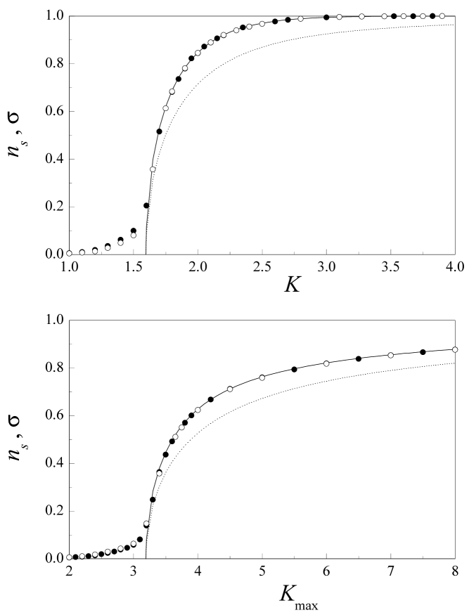
Figure 1: Upper panel: Numerical results for the fraction $n_{s}$ of synchronized oscillators in the case of constant couplings, $k_{i}=K$ for all $i$, with constant weights, $q_{i}=1$ for all $i$ (solid dots), and with uniformly distributed weights (open dots). Lower panel: The same, for the case of uniformly distributed couplings, $0<k_{i}<K_{\max}$. Full and dotted curves stand for the analytical calculation of $n_{s}$ and the collective amplitude $\sigma$, respectively.

The full curve represents the analytical estimate for the fraction of synchronized oscillators, defined from our analytical results as

$$n_{s}\equiv\int_{0}^{\infty}dk\int_{0}^{\infty}\ dq\int_{0}^{2\pi}d\psi\ n_{s}(\psi;k,q),$$ (43)

while the dotted curve is the analytical result for the collective amplitude $\sigma$, obtained from Eq. (24). Both $n_{s}$ and $\sigma$ are different from zero above Kuramoto’s critical coupling $K_{c}=2/\pi g(0)=2\sqrt{2/\pi}\approx 1.596$.

The agreement between numerical and analytical results is very good for $K>K_{c}$. Below the synchronization transition, on the other hand, we find a noticeable difference which, as advance above, is associated with the formation of synchronized clusters. This phenomenon is illustrated later. Note also that, in agreement with our discussion on the irrelevance of the distribution of weights when they are uncorrelated to couplings, solid and open dots above the transition fall over the same curve.

The lower panel of Fig. 1 displays analogous results for the case where couplings are uniformly distributed in the interval $(0,K_{\max})$. The corresponding distribution is $h(k)=K_{\max}^{-1}$ for $0<k<K_{\max}$, and $h(k)=0$ otherwise, and the synchronization transition takes place at $K_{\max}=2K_{c}\approx 3.192$. Again, the agreement between numerical and analytical results is very good above the transition, and the same kind of deviation is observed below it. Also, as expected, the distribution of weights $q_{i}$ has no effect on the fraction of synchronized oscillators.

A suitable illustration of the state of the system close to the synchronization transition, where analytical and numerical results differ from each other, is provided by a plot of the effective frequencies $\omega_{i}^{\prime}$ versus the natural frequencies $\omega_{i}$ of all oscillators in a given realization of the ensemble. In this kind of plot, a horizontal array of dots –corresponding to oscillators with different natural frequencies but the same effective frequency– reveals the presence of a synchronized cluster. Figure 2 displays such plots for the four cases already considered in Fig. 1. In the upper line, couplings are constant, $k_{i}=K=1.5$ for all $i$, while in the lower line they are uniformly distributed between $0$ and $K_{\max}=3$. In both cases, thus, the system is just below the synchronization threshold. The appearance of synchronized clusters near the center of the frequency distribution is apparent in the four plots.

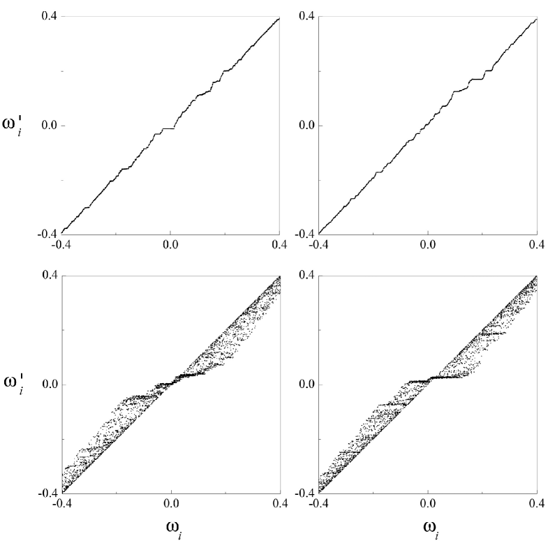
Figure 2: The effective frequency $\omega_{i}^{\prime}$ as a function of the natural frequency $\omega_{i}$ of individual oscillators in single realizations for constant coupling, $k_{i}=1.5$ for all $i$, with constant weights (upper right), and uniformly distributed weights (upper left), and for uniformly distributed couplings, $0<k_{i}<3$, with constant weights (lower right), and uniformly distributed weights (lower left). Only the central region of the frequency distributions is displayed.

Figure 2 shows again that, for a given distribution of couplings, there is little qualitative difference between the cases where the weights $q_{i}$ are either constant or distributed. On the other hand, we find that for oscillators with a given natural frequency, the effective frequencies are essentially identical in the case of constant couplings, but exhibit a substantial dispersion for distributed couplings. This difference can be understood by extrapolating our analytical results for the synchronization regime to the present situation, just below the transition. In fact, Eq. (20) implies that, for a given natural frequency, the effective frequency depends on $k_{i}$, so that we expect to have the same value of $\omega_{i}^{\prime}$ in the case of uniform coupling, and different values if couplings are distributed. It also predicts that the effective frequency of a given oscillator should be smaller than its natural frequency when the latter is larger than the synchronization frequency $\Omega$, and vice versa. We see from Fig. 2 that our numerical calculations, for which $\Omega\approx 0$, agree with such prediction.

Our previous results for the case of constant weights [9], which we do not reproduce here, suggest that the regime of frequency clustering is a finite-size effect due to fluctuations in the distribution of natural frequencies. An unusual accumulation of oscillators in a given frequency interval can trigger local entrainment for couplings below the transition to synchronization. Numerical results show that clustering becomes less important, with a smaller fraction of entrained oscillators, as the ensemble grows in size. In the limit of an infinitely large system, fluctuations should average out and synchronization should switch on at the analytically predicted threshold, with the formation of a macroscopic cluster. However, the fact the frequency clustering is still conspicuous in a relatively large ensemble as in our calculations seems to point out that this regime plays a relevant role in the collective dynamics of finite systems.

4.2 Weight-coupling anti-correlation

We turn now the attention to the case discussed in Section 3.3, where couplings and weights are correlated. As above, couplings are uniformly distributed on $(0,K_{\max})$, and the weight of each oscillator is given as function of its coupling through Eq. (40). We focus on the more interesting case of weight-coupling anti-correlation, where synchronization suppression is possible, so that we take $\lambda<0$. Results are thus presented in terms of the positive parameter $|\lambda|$. We recall that, in our analysis of infinitely large ensembles, Eq. (41) predicts the relation between $\lambda$ and $K_{\max}$ at the synchronization threshold. Figure 3 shows the region of the $(K_{\max},|\lambda|)$ parameter plane where synchronized states are possible. Synchronization is suppressed for small couplings and strong weight-coupling anti-correlation. In particular, it cannot occur for any $|\lambda|$ if $K_{\max}<2/\pi g(0)=4\sqrt{2/\pi}\approx 3.192$, or for any $K_{\max}$ if $|\lambda|>\pi g(0)/2=\sqrt{\pi/8}\approx 0.627$. Inserts in Fig. 3 illustrate the relation of effective and natural frequencies at several points in the parameter plane.

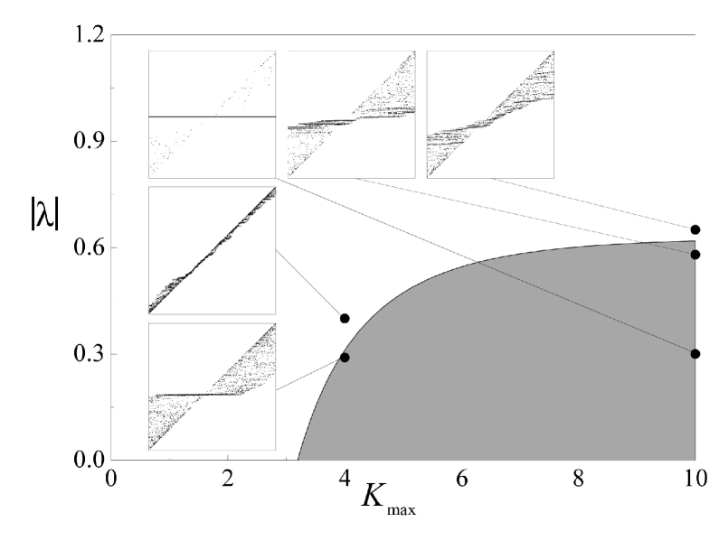
Figure 3: Synchronization region (gray shaded), obtained analytically for anti-correlated couplings and weights, Eq. (40), in the $(K_{\max},|\lambda|)$ parameter plane. The inserts show plots of individual effective frequencies versus natural frequencies (cf. Fig. 2), for single realizations of the system at the indicated points of the parameter plane. Scales in all the inserts vary from $-0.4$ to $0.4$ on both axes.

For small values of $|\lambda|$, the main effect of weight-coupling anti-correlation is to shift the synchronization transition to higher couplings. This is shown in Fig. 4, where the fraction of synchronized oscillators is plotted as a function of $K_{\max}$ for four values of $|\lambda|$. Full lines correspond to the analytical prediction, which again gives a very good description of the numerical results above the transition, at least for $|\lambda|=0.2$ and $0.4$. Dotted lines are plotted as a guide to the eye in the region preceding the synchronization transition. For $|\lambda|=0.6$, the systems is practically at the limit where synchronization becomes inhibited for any $K_{\max}$. The analytical transition point is strongly shifted to the right, but a considerable fraction of the ensemble is synchronized in clusters well below the transition. Note that a discrepancy between numerical and analytical results persists above the critical point. Finally, for $|\lambda|=1$, synchronization should be completely suppressed for infinitely large systems. In our numerical calculations, a small fraction of the ensemble –which grows with $K_{\max}$– is however synchronized.

Figure 4: The fraction $n_{s}$ of synchronized oscillators for the case of anti-correlated couplings and weights, as a function of $K_{max}$, for four values of $|\lambda|$. Full curves stand for the analytical prediction, and dotted curves are plotted as a guide to the eye in the region of frequency clustering.

It turns out that the quantities that characterize synchronization in the clustering regime –such as the fraction of synchronized oscillators, and the number of clusters– depend strongly on the value of $K_{\max}$. This is illustrated, for instance, by the two inserts of Fig. 3 corresponding to parameters just outside the synchronization region. For $K_{\max}=4$, clusters are small and relatively sparse, and most effective frequencies are close to the corresponding natural frequencies (all dots are near the diagonal). For $K_{\max}=10$, on the other hand, a substantial fraction of the ensemble around the center of the frequency distribution is entrained into clusters, and form massive groups extended over considerable intervals of natural frequencies. This effect can be understood taking into account that a fluctuation in the distribution of frequencies is more likely to give rise to a synchronized cluster if the involved oscillators have, on the average, larger couplings.

Figure 5: Upper panel: Fraction $n_{s}$ of synchronized oscillators as a function of $|\lambda|$, for $K_{\max}=4$. The full curve is the analytical prediction, and the dotted curve has been added as a guide to the eye in the clustering regime. Lower panel: The corresponding number of clusters, $C$. The dotted curve is a spline approximation.

A more quantitative illustration of this dependence on $K_{\max}$ is provided by the numerical results presented in Figs. 5 and 6. The upper panel of Fig. 5 shows the fraction $n_{s}$ of synchronized oscillators as a function of $|\lambda|$, for $K_{\max}=4$. The curve corresponds to the analytical prediction. For $|\lambda|$ larger than the critical value, $n_{s}$ decreases rapidly, such that only $2\%$ of the ensemble remains clustered for $|\lambda|\approx 1$. In the lower panel, we plot the corresponding number of clusters, $C$. Below the transition, in the synchronization region, $C\approx 1$. Around the transition point, the number of clusters increases abruptly, and reaches a maximum just below $C=20$, before beginning to decline for larger $|\lambda|$.

For $K_{\max}=10$, the behaviour of both $n_{s}$ and $C$ is qualitatively similar, but important quantitative differences are apparent. First, the fraction of synchronized oscillators in the clustering region is much higher and its decay is slower, with approximately $10\%$ of the ensemble still entrained into clusters for $|\lambda|\approx 1$. Second, the number of clusters at the transition grows above $C=60$, and the subsequent decay is extremely slow. For values of $|\lambda|$ twice as large as the critical point, $C$ remains practically as large as just above the transition.

Figure 6: As in Fig. 5, for $K_{\max}=10$.

5 Conclusion

In this paper, we have considered an ensemble of coupled phase oscillators where the strength of the interaction is generally different for each oscillator pair. This heterogeneity is represented by symmetric positive interaction coefficients $W_{ij}$ and, together with the distribution of natural frequencies $\omega_{i}$, adds diversity to the ensemble. Our main goal has been to show that Kuramoto’s theory for the synchronization transition of an infinitely large ensemble of globally coupled phase oscillators can be extended to the case of heterogeneous coupling, yielding exact results when the interaction coefficients can be factorized as $W_{ij}=k_{i}q_{j}$. The factors $k_{i}$ and $q_{i}$ turn out to be, respectively, the coupling strength of oscillator $i$ with the mean field generated by the ensemble, and the weight with which the same oscillator contributes to that mean field. The three attributes that characterize each oscillator, $\omega_{i}$, $k_{i}$, and $q_{i}$, are distributed over the ensemble according to a function $G(\omega,k,q)$ which, in general, introduces statistical correlations between them.

In the analysis of our results, we have paid particular attention to the effects of correlations between natural frequencies $\omega_{i}$, couplings $k_{i}$, and weights $q_{i}$. As it may have been expected, if the couplings and/or the weights of the oscillators which trigger synchronization –around the center of the frequency distribution– are relatively small, an overall larger coupling will be necessary to effectively have synchronized states. The effect of correlations between couplings and weights, on the other hand, is less obvious. We have found that a sufficiently strong anti-correlation between $k_{i}$ and $q_{i}$ is able to completely inhibit synchronization, in the sense that synchronized states are suppressed even in the presence of arbitrarily large couplings. In other words, if the mean field is strongly dominated by oscillators whose coupling is weak, and vice versa, the ensemble may be unable to display coherent collective oscillations.

As a validation of the analytical formulation, we have performed numerical calculations for ensembles of $10^{4}$ oscillators, with several combinations of the distribution of couplings and weights. Numerical and analytical results are in good overall agreement, except for a systematic departure in the parameter regions where the synchronization transition takes place. In these zones, numerical results reveal the existence of a regime of partial synchronization, where oscillators become entrained into several internally synchronized clusters. As the transition is approached, these clusters grow in size and, at the same time, they progressively aggregate with each other. Eventually, they collapse into a single cluster, which can be identified with the macroscopic fraction of synchronized oscillators predicted by the analytical formulation. Previous numerical results on a special case of the present system [9], seem to indicate that frequency clustering is a finite-size effect which disappears for infinitely large systems –where, precisely, the analytical approach is formulated. In finite ensembles, clusters may emerge from localized fluctuations in the distribution of frequencies and couplings, which trigger the mutual synchronization of a few oscillators.

The regime of clustering preceding the transition to synchronization found in our system, is reminiscent of a similar phenomenon well-known to occur in ensembles of coupled chaotic elements [10, 11, 12, 5]. In the present case, heterogeneity in the ensemble replaces chaotic dynamics as the factor which counteracts the effects of coupling and gives origin to the transition. In spite of the fact that it may disappear in the thermodynamical limit, clustering remains the richest dynamical regime of oscillator ensembles because of its complexity and diversity [13].

In connection with chaotic systems, it would be interesting to study whether the introduction of coupling heterogeneity in ensembles of chaotic dynamical elements have effects similar to those described here for the synchronization transition of phase oscillators. More complex individual dynamics are also expected to give rise to new collective phenomena, such as amplitude effects. Distributed couplings $k_{i}$ and weights $q_{i}$ can be straightforwardly incorporated to standard models of interacting chaotic systems [5]. For instance, linear heterogeneous coupling between $N$ chaotic elements whose individual dynamics is governed by the equation $\dot{\bf x}={\bf f}({\bf x})$ may be introduced as

$$\dot{\bf x}_{i}={\bf f}({\bf x}_{i})+k_{i}({\bf X}-{\bf x}_{i}),$$ (44)

$i=1,\dots,N$, with ${\bf X}=N^{-1}\sum_{i}q_{i}{\bf x}_{i}$. Finally, let us point out that Kuramoto’s theory has been extended, at least partially, to study the synchronization properties of ensembles formed by other kinds of dynamical elements, in particular, by active rotators [14, 15]. Consideration of such ensembles with the kind of heterogeneous coupling studied here would be a natural continuation of the present work.

References

- [1] N. Wiener, Cybernetics, or Control and Communication in the Animal and the Machine (MIT Press, Cambridge, 1948).
- [2] A. T. Winfree, Biological rhythms and the behavior of populations of coupled oscillators J. Theor. Biol. 16 (1967) 15.
- [3] A. T. Winfree, The Geometry of Biological Time (Springer, Berlin, 1980).
- [4] Y. Kuramoto, Chemical Oscillations, Waves, and Turbulence (Springer, Berlin, 1984).
- [5] S. C. Manrubia, A. S. Mikhailov, and D. H. Zanette, Emergence of Dynamical Order. Synchronization Phenomena in Complex Systems (World Scientific, Singapore, 2004).
- [6] A. S. Mikhailov and V. Calenbuhr, From Cells to Societies. Models of Complex Coherent Action (Springer, Berlin, 2002).
- [7] H. Daido, Population dynamics of randomly interacting self-oscillators, Prog. Theor. Phys. 77 (1987) 622.
- [8] H. Daido, Quasientrainment and slow relaxation in a population of oscillators with random and frustrated interactions, Phys. Rev. Lett. 68 (1992) 1073.
- [9] G. H. Paissan and D. H. Zanette, Synchronization and clustering of phase oscillators with heterogeneous coupling, Europhys. Lett. 77 (2007) 20001.
- [10] K. Kaneko, Clustering, coding, switching, hierarchical ordering, and control in a network of chaotic elements, Physica D 41 (1990) 137.
- [11] D. Golomb, D. Hansel, B. Shraiman and H. Sompolinsky, Clustering in globally coupled phase oscillators, Phys. Rev. A 45 (1992) 3516.
- [12] D. H. Zanette and A. S. Mikhailov, Condensation in globally coupled populations of chaotic dynamical systems, Phys. Rev. E 57 (1998) 276.
- [13] A. S. Mikhailov, D. H. Zanette, Y. M. Zhai, I. Z. Kiss, and J. L. Hudson, Cooperative action of coherent groups in broadly heterogeneous populations of interacting chemical oscillators, Proc. Nat. Acad. Sci. USA 101 (2004) 10890.
- [14] H. Sakaguchi and Y. Kuramoto, A soluble active rotator model showing phase transitions via mutual entrainment, Prog. Theor. Phys. 76 (1986) 576.
- [15] C.J. Tessone, A. Scirè, R. Toral, and P. Colet, Theory of collective firing induced by noise or diversity in excitable media, Phys. Rev. E 75 (2007) 016203.