Nonlinearizing linear equations to integrable systems including new hierarchies with nonholonomic deformations

Abstract

We propose a scheme for nonlinearizing linear equations to generate integrable nonlinear systems of both the AKNS and the KN classes, based on the simple idea of dimensional analysis and detecting the building blocks of the Lax pair. Along with the well known equations we discover a novel integrable hierarchy of higher order nonholonomic deformations for the AKNS family, e.g. for the KdV, the mKdV, the NLS and the SG equation, showing thus a two-fold universality of the recently found deformation for the KdV equation [6].

Running Title: Nonlinearizing linear equations

PACS: 02.30.lk, 02.30.jr, 05.45.Yv, 11.10.Lm

I. INTRODUCTION

In spite of the significant achievements in the theory of integrable systems over the last fifty years, it remains a mystery: what is integrable nonlinearity, i.e. how to identify a priory those nonlinear terms which make an equation integrable.

Nevertheless one notices that, although integrable equations can be of diverse types, the integrability filters out the nonlinearity to some specific forms, as evident from the well known equations like the nonlinear Schrödinger (NLS) equation, the derivative NLS (DNLS), the Korteweg-de Vries (KdV) equation, the modified KdV (mKdV), the sine-Gordon (SG) equation etc.[1]. Moreover, all such integrable nonlinear PDEs exhibit exact soliton solutions, localized and stable form of which is believed to be due to a fine balance between their linear dispersive and nonlinear terms. Therefore it may not be unexpected to expect that a linear PDE, the dispersive part of which would balance the nonlinear term, should have the information of the integrable nonlinearity hidden in it. Consequently, there must be a scheme for nonlinearizing linear equations for generating integrable systems. However attacking this anti-intuitive question directly seems to have been avoided in the literature, although the Ablowitz-Kaup-Newell-Segur (AKNS) scheme [1] and the celebrated Sato construction [2] aimed around this line and a recent attempt came close to it [3].

We propose here a direct but easy scheme for nonlinearizing the linear equations

$$iq_{t}=q_{xx},\ q_{t}=q_{xxx},\ \theta_{xt}=0,$$ (1)

etc. together with their conjugates, which are in fact the linearized parts of the well known equations like the NLS, the DNLS, the KdV, the SG etc. Our aim is to generate first the known integrable systems, proving thus the effectiveness of our alternative scheme based on a simple physical idea of dimensional analysis and then, continuing the process search for new integrable nonholonomic deformations for all known equations.

It is evident that the direct nonlinear extension of a linear equation is not unique, since it alone can not identify the integrable nonlinearity and one needs some extra structure for filtering out the integrable cases. Our strategy therefore is to stick from the beginning to a Lax pair, a property inherent to all integrable systems, by defining a pair of naive Lax operators $U^{(l)},V^{(l)}$ for the linear system itself and then nonlinearize them to a genuine pair $(U,V)$, which finally generate the nonlinear integrable equation through their flatness condition

$$U_{t}-V_{x}+[U,V]=0$$ (2)

.

It is true that several sophisticated formal methods like the prolongation technique, the Painlevé truncation [4], the Sato theory [2], the AKNS method [1] etc. are available in the literature for constructing the Lax pair of a nonlinear integrable equation. However our alternative construction, based on a fundamental concept of dimensional analysis, is perhaps the simplest and the most physical one. Exploiting only the scaling dimensions and identifying the constituent building blocks of the Lax operators, hidden already in the linear equations, we can construct a Lax pair quite easily to any higher order for both the AKNS [1] and the Kaup-Newell (KN) [5] spectral problems. Interestingly, by regulating the scaling dimension of the field we can generate uniquely both the NLS and the DNLS equations, starting from the same linear Schrödinger (LS) equation. Finally as an important application we discover new integrable hierarchies of nonholonomic deformations for the well known equations like the KdV, the mKdV, the NLS, the SG etc. The nonholonomic deformation in this field theoretical context is given by some differential constraints on the deforming function. A recently discovered 6-th order integrable KdV (6KdV) equation, attracting much attention [6, 7, 8], happens to be the lowest order deformation of this kind for the KdV equation. We are able to generalize here not only the earlier result on the deformed KdV and the 6KdV by unveiling a novel hierarchy of their higher order deformations, but also to show the universality of such perturbations, by discovering integrable nonholonomic deformations for all members of the AKNS family, including their higher order integrable hierarchies, a task termed as highly desirable but quite impossible in a recent study [7]. Interestingly, such deformed integrable systems can be represented also as known nonlinear equations with additional perturbative terms subjected to differential constraints. Such perturbations, contrary to the usual belief, not only preserve the integrability of the original equation but also yield richer properties.

Nonlinear integrable systems like the NLS, the mKdV and the SG equations with various perturbations appear in many physical situations, e.g. fluxons in Josephson junction, parametrically driven damped molecular chain, nonlinear optical fiber communication, ferromagnet in variable magnetic field, nonlinear Faraday resonance etc. [9]. However in almost all these perturbed systems the integrability - the most cherishable property of a nonlinear system - is usually lost. As a result all their related precious properties like higher conserved quantities, exact soliton solutions, elastic scattering of solitons etc., enormously useful in physical applications, are also lost. Therefore constructing integrable perturbed systems, preserving their complete integrability and exact soliton solutions, is a challenging physical problem, which we are able to solve here to certain extend.

Our integrable perturbed equations exhibit the usual exact N-soliton solutions, but with an unusual accelerated or decelerated motion. Recall that the standard solitons move with a constant velocity and behave like particles undergoing elastic collisions with other solitons, which have been of significant importance and application in various physical problems. In the present context of integrable perturbed equations the accelerated solitons behave like particles under external forces. They are subjected to perturbations, which are themselves solitonic in nature. In fact the time-dependent asymptotic value of such a perturbing function acts like a force sitting at the space boundaries and controlling the motion of the field soliton, depending on the nature of which the soliton can accelerate or decelerate.

Accelerated solitons appear in many physical models like inhomogeneous plasma [10] , information transfer in the DNA chain [11] , transport of solitons and bubbles [13] etc. Therefore the present integrable models with exact accelerating solitons showing elastic soliton scattering [12] could find applications in practical situations.

The arrangement of the paper is as follows. Sec. II introduces our nonlinearization scheme. Generation of specific nonlinear integrable systems is presented in Sec. III. New integrable nonholonomic deformations of the AKNS system are detailed in Sec. IV, with the concrete examples given in Sec. V. In Sec. VI the present result is listed and compared with the existing ones. Sec. VII is the concluding section followed by the bibliography.

II. THE NONLINEARIZATION SCHEME

Combining field $q$ and its conjugate $r$ in a matrix as $U^{(0)}=q\sigma^{+}+r\sigma^{-}$, where $\sigma^{\pm}={1\over 2}(\sigma^{1}\pm i\sigma^{2})$ and $\sigma^{a},a=1,2,3$ are standard $2\times 2$-Pauli matrices, we can clearly express our starting linear dispersive equations (1) as  $iU^{(0)}_{t}=\sigma_{3}U^{(0)}_{xx},\ \ U^{(0)}_{t}=U^{(0)}_{xxx},$ etc. These linear equations in turn can be expressed by easy observation as a linear flatness condition $U^{(l)}_{t}-V^{(l)}_{ix}=0$, which is defined by ignoring the nonlinear commutator term between Lax operators. This naturally identifies the pairs of naive Lax operators $(U^{(l)},V_{i}^{(l)}),\ i=2,3,\dots$ for the consecutive higher order linear equations as

$$U^{(l)}=i\lambda\sigma_{3}+iU^{(0)},\ \ \ \ \mbox{and}\ \ V^{(l)}_{2}=\sigma_{3}U^{(0)}_{x},\ \ V^{(l)}_{3}=iU^{(0)}_{xx},$$ (3)

etc. with $\rm{tr}U^{(l)}=\rm{tr}V^{(l)}_{i}=0,\ i=2,3,\ldots$, since $\rm{tr}\sigma_{3}=\rm{tr}U^{(0)}=\rm{tr}(\sigma_{3}U^{(0)})=0$. The significance of parameter $\lambda$, which enters here only as an additional constant and can be ignored without any loss, will become clear in the process.

The Next important point is to detect the scaling dimension of the Lax operators as well as to identify their crucial building blocks (BB), existence of which seem to have been overlooked in most of the work including the AKNS construction.

A. Scaling dimension and building blocks of the Lax pair

We consider length $L$ as the fundamental dimension and from the linear evolution equation with $N$-th order dispersion: $q_{t}=q_{\underbrace{xx\dots x}_{N}}$ read out the dimension $[\cdot]$ of time as $[T]=L^{N}$. The Lax operators, generating infinitesimal space and time translations, as evident from the Lax equations $\Phi_{x}=U\Phi,\ \Phi_{t}=V\Phi$, naturally should have the scaling dimensions (SD) as $[U]=L^{-1},\ [V_{N}]=[T]^{-1}=L^{-N}.$ Assuming that the linear Lax pair $U^{(l)},V^{(l)}_{N}$ share the same scaling dimensions as well as the same building blocks as their nonlinear counterpart, we find from the explicit structure (3), the SD of their constituent elements as $[\lambda]=[U^{(0)}]=L^{-1}$ and at the same time identify the building blocks (BB) for both the Lax operators as the set $\{\ \lambda,U^{(0)}\ \}$ and its x-derivatives: $U^{(0)}_{x},U^{(0)}_{xx},$ etc. , which enter in their construction linearly. Our crucial conjecture is that these linear Lax pair can be nonlinearized by adding all possible nonlinear combinations of the same BB, guided by the dimensional argument. Note that, the condition $[U^{(0)}]=L^{-1}$ fixes the SD for the field in this case as $[q]=[r]={L}^{-1}$. However, since a linear equation as such can not put any restriction on the SD of its fields, this input is not unique and we show below that a different fixation of the SD for the field would lead to another construction of the Lax pair.

Recalling that a nonlinear variable change can generate from a given integrable system other gauge equivalent equations [14], we concentrate here only on fundamental integrable equations like NLS, KdV DNLS etc. belonging to the AKNS or the KN family, while the gauge equivalent systems can be obtained trough simple transformations.

III. GENERATION OF NONLINEAR INTEGRABLE SYSTEMS

The dimension of the field $[q]$ and its conjugate $[r]$ as well as $[\lambda]$, which are not fixed by the starting linear equations (1), should be given in our nonlinearization scheme as input. We show that for $[q]=[r]=[\lambda]=L^{-1}$, we get the AKNS systems, while $[q]=[r]=[\lambda]=L^{-\frac{1}{2}}$ yields the KN hierarchy.

A. AKNS integrable hierarchy

We consider first the case $[q]=[r]=[\lambda]=L^{-1},$ which gives through the above construction: $[U^{(0)}]=[U^{(l)}]=L^{-1}$. We intend to construct now the space-Lax operator $U(\lambda)\in sl(2),\rm{tr}U(\lambda)=0$, naturally with $[U(\lambda)]=L^{-1}$, out of $U^{(l)}$ by using the BB: $\{\lambda,U^{(0)}\}$. Therefore the only possibility left from the dimensional argument, which only allows summation of the terms having the same dimension, is to take $U(\lambda)=U^{(l)}=i(\lambda\sigma_{3}+U^{(0)}),$ recovering thus the well known AKNS Lax operator [1] uniquely. However for constructing the corresponding time-Lax operator $V_{2}(\lambda)\in sl(2)$ with $\rm{tr}V_{2}(\lambda)=0$ and SD: $L^{-2},$ in addition to $V^{(l)}_{2}=\sigma_{3}U^{(0)}_{x},$ nonlinear terms $V^{(nl)}_{2}$ with the same SD: $L^{-2}$ are to be constructed out of the same BB $\{\lambda,U^{(0)}\}$, through their nonlinear products and powers like $\lambda^{2},\lambda U^{(0)},(U^{(0)})^{2},$ following the dimensional argument. Note that since $[\partial_{x}]=L^{-1}$, the derivative term $U^{(0)}_{x}$ can appear only in the linear part, again from the dimensional analysis.

Therefore this set of nonlinear terms is sufficient to construct the nonlinear part of the time-Lax operator: $V^{(nl)}_{2}=i(k_{2}\lambda^{2}\sigma_{3}+k_{1}\lambda U^{(0)}+k_{0}\sigma_{3}(U^{(0)})^{2})$, upto the integer coefficients $k_{n},n=0,1,2$. Note that fixing the dimensionless integers $k_{n}$ with different terms in $V_{2}(\lambda)=V^{(l)}_{2}+V_{2}^{(nl)}$ goes beyond the scope of the dimensional argument, which however is achieved from the flatness condition of $U(\lambda),V_{2}(\lambda)$, yielding several consistency relations at different powers of $\lambda$. Interestingly, the number of such relations obtained is just sufficient to determine the numerical coefficients of all the terms without any ambiguity. For example, it is easy to check that, the condition (2) for $U(\lambda),V_{2}(\lambda)$ yields three consistency conditions at three different powers of $\lambda^{n},\ n=0,1,2,$ of which the condition at $n=0$ fixes $k_{0}=-1$, that at $n=1$ fixes the integer $k_{1}=2$, while $n=2$ gives the relation $k_{2}=k_{1}$. Thus all the integer coefficients are obtained exactly, determining the structure of the nonlinear part unambiguously as

$$V^{(nl)}_{2}=2i\lambda^{2}\sigma_{3}+2i\lambda U^{(0)}-i\sigma_{3}(U^{(0)})^{2},$$ (4)

with $\rm{tr}V^{(nl)}_{2}=0,$ which constructs the complete time-Lax operator uniquely as $V_{2}(\lambda)=V^{(l)}_{2}+V_{2}^{(nl)}$ . Note that the asymptotic solutions of the Lax equation giving $e^{\pm i\lambda x}$ clarifies the physical meaning of parameter $\lambda$ as the momentum and justifies the choice of its SD: $L^{-1}$. At the final step we obtain the integrable nonlinear equation we are searching for, again from the flatness condition, where a nonlinear term $2\sigma_{3}(U^{(0)})^{3}$ appears now in addition to the initial linear equation $iU^{(0)}_{t}=\sigma_{3}U^{(0)}_{xx}$. For $r=\pm q^{*}$ this nonlinear term reduces to $\pm 2|q|^{2}q$, which together with the starting LS equation yields finally the integrable NLS equation, completing our nonlinearization process.

The next higher order linear equation $q_{t}=q_{xxx}$ follows a similar procedure in the nonlinearization process. The space-Lax operator being the same, one has to build only the time-Lax operator $V_{3}(\lambda)$ by adding to the naive operator $V^{(l)}_{3}=iU^{(0)}_{xx}$ a nonlinear part $V^{(nl)}_{3}$ with SD $L^{-3}$, which is to be constructed again from the same BB : $\{\lambda,U^{(0)}\}$ and its derivative $\ U^{(0)}_{x},$ following our conjecture. Observe that the derivative term can appear now in the nonlinear part on dimensional ground. By all possible nonlinear combinations as powers and products of the BB with total SD = $L^{-3}$ and maintaining $\rm{tr}V_{3}(\lambda)=0$, we can, similar to the above, construct uniquely :

$$V_{3}^{(nl)}=-4i\lambda^{3}\sigma_{3}+2\sigma_{3}(-U^{(0)}_{x}+i(U^{(0)})^{2})\lambda-4iU^{(0)}\lambda^{2}+2i(U^{(0)})^{3}-[U^{(0)},U^{(0)}_{x}],$$ (5)

yielding finally $V_{3}(\lambda)=V^{(l)}_{3}+V^{(nl)}_{3}$. The flatness condition of the pair $U(\lambda),V_{3}(\lambda)$ fixes again the integer coefficients in different terms of (5) and yields the integrable equation, by adding only one nonlinear term $\ (U^{(0)})^{2}U^{(0)}_{x}\$ to the starting linear dispersive equation $\ U^{(0)}_{t}=U^{(0)}_{xxx}\$. For $r=\kappa=const.,\ q=u$ the nonlinear term reduces to $\kappa 6uu_{x}$, while for $r=q=v$ to $6v^{2}v_{x}$, generating thus the well known integrable KdV and mKdV equations, from the third order linear equation we started with.

Similarly one can continue building the hierarchy of integrable equations, starting from the arbitrary higher order linear equation $q_{t}=q_{{xx\dots x}}$ and nonlinearize it following the procedure as above and using the same BB and similar dimensional argument, as we have conjectured. Since the space-Lax operator $U(\lambda)$ remains the same, the task is to construct only the time Lax operator $V_{N}(\lambda)$ with the SD $L^{-N}$ for arbitrary $N$, out of the same BB: $\{\lambda,U^{(0)}\}$ by all possible combinations like

$$(\lambda)^{k}(\frac{\partial}{\partial x})^{l}(U^{(0)})^{m}$$ (6)

with the dimensional constraint $k+l+m=N$. It is easy to check that this partitioning of $N$ determines the total number of terms that can appear in $V_{N}(\lambda)$ as $L=1+\frac{1}{2}N(N+1)$, which interestingly tallis with our result obtained above, giving $L=4$ for the NLS with $N=2$ and $L=7$ for the KdV and mKdV with $N=3$. Thus we can estimate the exact number of terms that should appear in any higher order Lax operator, without even calculating their explicit form. This unique feature of our nonlinearization scheme, obtained from the dimensional argument and the identification of the BB, is absent in all other available methods.

B. Comparison with the AKNS scheme

It is true that, though we have presented a simple and original scheme for nonlinearizing linear equations to integrable systems, based on the dimensional analysis and using the building blocks of the Lax pair, we could reproduce so far only the known integrable equations, which are obtainable also through the AKNS scheme [1]. In-spite of this fact and before presenting our new result, we intend to show that in comparison with the AKNS proposal [1], the construction of time-Lax operator $V_{N}(\lambda)$, vital in generating integrable equations, is significantly simpler in the present scheme.

Recall firstly, that in the AKNS method one starts with a given nonlinear field equation and not from its linearized version, as done here.

Secondly, for obtaining the explicit form of $V_{N}(\lambda)$ in the AKNS method, one has to expand it in the powers of spectral parameter: $V_{N}(\lambda)=\sum_{n=1}^{N}=\lambda^{n}V^{(n)}$, where $V^{(n)},n=1,2,\ldots$ are $N$ number of $2\times 2$ unknown matrices with $4N$ number of unknown functions, some of them being complex. In our construction on the other hand, the unknown coefficients are only $N$ in number and moreover they are only real integers. This is because we have already identified the building blocks of the Lax operators made up from parameter $\lambda$, a known matrix $U^{(0)}$ and its derivatives, and the dimensional argument, which is our key ingredient, guides us to collect them in the right combination.

Thirdly, in the AKNS scheme the $4N$ unknown functions are to be determined by solving different partial differential equations. Our $N$ unknowns being only real integers are obtained from simple algebraic equalities.

This simplicity of our scheme becomes more evident for higher values of $N$, where $V_{N}$ contains $L=1+\frac{1}{2}N(N+1)$ number of terms. Note that determining a priori the number of terms that should be present in any $V_{N}$, as we have shown above is again easy in our scheme but not in the AKNS.

Fourthly, while for the KN spectral problem the AKNS type direct expansion becomes even more complicated, our scheme covers the KN system in an unified way. Just a change in the scaling dimension of the field switches our scheme from the AKNS to the KN family, as we demonstrate below.

Finally, as an important application we discover new integrable hierarchies of nonholonomic deformations for all members of the AKNS family (see Sec. V), systematic account of which is absent in AKNS [1].

C. KN integrable hierarchy

Our nonlinearization scheme , as we show here, is universally applicable for generating the KN hierarchy, which is not readily available in the literature due to its apparent complicacy.

We follow again the same line of argument, making a slight change in the input of the SD of the field as $[q]=[r]=[\lambda]=L^{-\frac{1}{2}}$. This small deviation however dramatically changes the outcome and resolves the puzzle we faced in generating uniquely two different nonlinear equations, namely the NLS and the DNLS equations, starting from the same linear LS equation.

Note that the SD of the linear Lax operator has been changed now to $[U^{(l)}]=L^{-\frac{1}{2}}$, while that for the genuine space Lax operator must always be $[\tilde{U}(\lambda)]=L^{-1}$. Therefore the nonlinearization induced by the dimensional argument should give $\tilde{U}(\lambda)=\lambda U^{(l)}=i\lambda^{2}\sigma_{3}+i\lambda U^{(0)}$, which reproduces correctly the well known KN Lax operator [5]. Note that, in principle, one can also add on dimensional ground. a term like $i\sigma_{3}(U^{(0)})^{2}$ to this Lax operator. However, such an addition does not produce any independent equation that are not derivable from those obtained without its addition.

For constructing the corresponding time-Lax operator $\tilde{V}_{N}(\lambda)$ through our nonlinearization, one should remember that the situation is a bit different here, since though the dimension of $\tilde{V}_{N}(\lambda)$ must remain as $L^{-N}$, the SD of its BB: $\{\lambda,U^{(0)}\}$ has been changed.

Let us consider first the case with $N=2$ and start again from the linear Schrödinger equation. We repeat the above procedure for the NLS case, but with the present change in the dimension of the BB, which should lead to the construction $\tilde{V}_{2}(\lambda)=\lambda V_{2}^{(l)}+V^{(nl)}(\lambda)$ due to the dimensional constraint $L^{-2}$, where $V_{2}^{(l)}=\sigma_{3}U^{(0)}_{x}$ is the naive linear operator as in (3). The nonlinear part $V^{(nl)}(\lambda)$ should be constructed therefore by nonlinear combinations of the BB with dimension

$$L^{-2}=[\lambda][(U^{(0)})^{3}]=[\lambda^{2}][(U^{(0)})^{2}]=[\lambda^{3}][U^{(0)}]=[\lambda^{4}].$$ (7)

Note again that though terms like $i\sigma_{3}(U^{(0)})^{4},\ [U^{(0)},U^{(0)}_{x}]$ match in dimensionality and hence can also be added, they only yield equations that are derivable from those, obtained without their addition. This identification together with $\tilde{V}_{2}(\lambda)\in sl(2),\ \rm{tr}\tilde{V}_{2}(\lambda)=0,$ constructs the time-Lax operator

$$\tilde{V}_{2}(\lambda)=(\sigma_{3}U^{(0)}_{x}+i(U^{(0)})^{3})\lambda-i\sigma_{3}(U^{(0)})^{2}\lambda^{2}+2iU^{(0)}\lambda^{3}+2i\sigma_{3}\lambda^{4},$$ (8)

uniquely , with the integer coefficients fixed as above from the consistency condition. This condition generates also the nonlinear equation with the integrable nonlinearity $i((U^{(0)})^{3})_{x}$, which for $r=\pm q^{*}$ adds a term $\pm 2(|q|^{2}q)_{x}$ to our starting LS equation $iq_{t}-q{xx}=0,$ yielding the DNLS equation, as required.

Similarly the higher order linear equations we considered above nonlinearize now to a different set of integrable equations belonging to the KN hierarchy, due to the changed SD of the BB. Without giving the details we just mention, that the construction, though a bit tedious, is quite similar and straightforward and given again in the form (6), with the total number of terms appearing in $\tilde{V}_{N}(\lambda)$ as $\tilde{L}=1+N^{2}$, with arbitrary $N$ . Note that this number of terms $\tilde{L}$, resulting from the new SD constraint: $\frac{1}{2}(k+m)+l=N$, is much higher than the number $L$ appearing in its AKNS counterpart, showing why the KN systems are more complicated than those of the AKNS. Check that $N=2$ gives $\tilde{L}=5$ as we have obtained above for the DNLS case.

IV. NEW INTEGRABLE HIERARCHIES FOR THE AKNS FAMILY WITH NONHOLONOMIC DEFORMATIONS

Note that the emphasis in the above nonlinearization scheme is to construct the time-Lax operator $V_{N}(\lambda)=V^{(l)}_{N}+V^{(nl)}_{N}(\lambda),$ by building up the nonlinear part involving positive powers of $\lambda$ and confining to the elements only from the identified building block $U^{(0)}=q\sigma^{+}+r\sigma^{-}$ , which means to construct the nonlinear combinations of the same basic fields $q,r$ and their derivatives. Now we intend to extend this construction further by going beyond the conjecture of the BB and introducing new perturbative functions with SD $L>N$. Thus keeping $U(\lambda)$ same as above, we add a nonlinear deformation $V^{(def)}_{N}(\lambda)$ to the $V_{N}(\lambda)$ by including negative powers of $\lambda^{-n},n=1,2,\ldots$ in the dimensional argument, which we have ignored so far. This simple extension, as we show, would discover a completely new class of integrable perturbed equations with hierarchy of higher order nonholonomic deformations. Thus it creates a novel two-fold integrable hierarchy [12] by adding a deformation hierarchy to each of the known AKNS hierarchy. The well known equations like the NLS, the KdV, the mKdV and the SG can be deformed by perturbing functions with higher and higher order nonholonomic constraints, preserving the original integrability. The present result thus shows a two-fold universality for the nonholonomic deformations, found recently for the KdV equation [6, 7, 8], since one can cover now the entire AKNS family , originating from this single model, and at the same time can discover a new integrable deformation hierarchy for each members of this family.

It should be noted in this context, that the use of negative powers of the spectral parameter in the time-evolution operator was considered also in some earlier occasions in the long history of integrable systems. However this was either limited [1, 15], partial [16] or camouflaged [17]. The novelty of our result lies in the fact, that within this extremely well studied field we could discover in a simple way a class of new integrable systems with a novel two-fold integrable hierarchy, which can be interpreted as perturbed equations with integrable nonholonomic constraints. In this construction of the time-Lax operator, we do not confine to the BB, which involve only the basic fields, but include a series of new perturbing functions, each influencing the basic field. This situation can simulate an interesting device for controlling the basic solitons through multiple intervention, though remaining within the scenario of the exact solvability. Such an idea was partially realized in the fiber optics communication through doped media [18].

For presenting our new equations we start with $V_{2}(\lambda)$ for the AKNS system constructed above and deform it first by $V^{(def)}(\lambda)=\frac{i}{2}\lambda^{-1}G^{(1)}$, with a matrix function $G^{(1)}$ with $\rm{tr}G^{(1)}=0$ and SD $L^{-3}$. Since our intention is to introduce new perturbing function $g$ into the system, we derive from the flatness condition its structure as an integrable deformation of the second-order AKNS equation:

$$iq_{t}-q_{xx}-2(qr)q=g,$$ (9)

with the perturbing function, given by the matrix element $g=G^{(1)}_{12}$, subjected to the nonholonomic differential constraint:

$$G^{(1)}_{x}=i[U^{(0)},G^{(1)}].$$ (10)

Remarkably, we can include further perturbation into the system, which would interact with the basic field as well as with the initial perturbation. This process can also be viewed as putting higher order differential constraint on the original perturbation. To achieve this higher perturbation we extend $V^{(def)}(\lambda)$ with another deforming term $\frac{i}{2}\lambda^{-2}G^{(2)}$, where $G^{(2)}$ is a matrix function of SD $L^{-4}$. Integrability condition (2) now leads to a further deformation of (9) given by the higher order constraint

$$G^{(1)}_{x}=i[U^{(0)},G^{(1)}]+i[\sigma_{3},G^{(2)}],\ G^{(2)}_{x}=i[U^{(0)},G^{(2)}].$$ (11)

Generating such higher order integrable perturbations can be continued recursively by adding in $V^{(def)}(\lambda)$ more and more terms as $\frac{i}{2}\lambda^{-j}G^{(j)},j=1,2,\ldots n,$ with arbitrary $n$. New matrix functions $G^{(j)}$ have the scaling dimension $j+2$ anf $\rm{tr}G^{(j)}=0$. This would result to a new integrable hierarchy of nonholonomic deformations for (9), given recursively as

$$G^{(1)}_{x} = i[U^{(0)},G^{(1)}]+i[\sigma_{3},G^{(2)}],\ \ldots\ ,$$

$$G^{(n-1)}_{x} = i[U^{(0)},G^{(n-1)}]+i[\sigma_{3},G^{(n)}],$$

$$G^{(n)}_{x} = i[U^{(0)},G^{(n)}],$$ (12)

which clearly reduces to (10) for $n=1$ and to (11) for $n=2$.

Exactly in a similar way we can build up the hierarchy of integrable perturbations for each member in the known AKNS hierarchy of higher nonlinear equations, which would lead thus to a novel two-fold integrable hierarchy. In one the same nonlinear equation is perturbed by a function with increasingly higher order differential constraints and in the other all different higher nonlinear equations are deformed by the same perturbing function.

The most important fact about the hierarchies of all perturbed equations thus generated is that, they are completely integrable systems and are exactly solvable by the inverse scattering method (ISM), yielding $N$- soliton solutions. This follows from the fact that, for constructing such nonholonomic deformations, we have started from the Lax pair, keeping the space-Lax operator $U(\lambda)$ same as the original one, while deforming the time-Lax operator $V(\lambda)$. Therefore the scattering problem, which is central to the ISM remains the same, while the time evolution of the spectral data only gets changed for the deformed models. Consequently, in such perturbed systems along with the exact soliton solution for the basic field we can find the exact solution for the perturbing function, which intriguingly takes also the solitonic form. Moreover, one can analytically study the soliton dynamics as well as the scattering of multiple solitons, a task impossible to carry out under usual perturbation with a known function. It is of significant practical importance that, though in such perturbed integrable systems, the exact ISM is applicable for extracting the soliton solution, we can bypass this involved and lengthy procedure and achieve the same result by taking the well-known soliton solutions of the undeformed system and deforming them by suitably choosing their time-evolution, given by the deformed soliton velocity [12].

Remarkably, a perturbed soliton in the present set up behaves like a particle driven by a force and exhibits an accelerated or decelerated motion, depending on the nature of the deformation. Note that unlike known situations [19] the variable soliton velocity occurs here without any apparent inhomogeneity and within the framework of an isospectral flow.

V. NEW INTEGRABLE EQUATIONS: SIMPLE EXAMPLES

Using the above construction suitable for equations belonging to the AKNS spectral problem we can now analyze in detail the new class of integrable perturbations for all members of this family, namely the KdV, the mKdV, the NLS and the SG equations. In particular constructing the matrix Lax pair for each of them we can find the explicit form for all those deformed equations, explore their higher deformations and most importantly, obtain their exact N-soliton solutions.

Along with these perturbed equations we can also study their two-fold integrable hierarchies, as developed above. However we present here only the simplest equations in this hierarchy, which are the most important cases involving the perturbation of the well known equations and represent the lowest order nonholonomic deformation, obtained from (12) with $n=1$ or $2$.

A. Integrable perturbation of the KdV equation

Recent findings of the integrable nonholonomic deformation of the KdV equation, equivalent to a 6th-order KdV equation [6], which apparently contradicts the accepted notion of nonexistence of any even-order equation in the KdV hierarchy, arose considerable interest [7, 8]. However, the exact integrability of this system through AKNS type matrix Lax operator or its exact N-soliton solutions through the ISM could not be established. Consequently, the integrable hierarchies allowed by this system as well as the dynamics of the solitons, including their nature of scattering could not be explored.

We on the other hand have developed the formalism in Sec. IV for constructing AKNS type Lax operators for all of its members with nonholonomic deformations, which should solve completely the remaining unsolved aspects of the deformed KdV equation, as we show below.

Recall that in the AKNS hierarchy KdV type equations appear at $N=3$ level, for which we have derived explicitly the time-Lax operator $V_{3}(\lambda),$ through our nonlinearization scheme. Now we intend to deform this Lax operator by an additional $V^{(def)}(\lambda)$ matrix, which would result to a deformed 3rd-order AKNS equation

$$q_{t}-q_{xxx}-6(qr)q_{x}=g_{x},$$ (13)

with the multiple nonholonomic constraints as in (12) on the deforming matrices $G^{(j)}$, having higher scaling dimension: $j+3$. For deriving the perturbed KdV equation we have to make the standard reduction $r=1$ , $q=u$ in (13) to yield

$$u_{t}-u_{xxx}-6uu_{x}=g_{x}(t,x).$$ (14)

For fixing now the lowest order constraint on the deforming function, we have to add two terms with $n=1,2$ to $V^{(def)}(\lambda)=\frac{i}{2}(\lambda^{-1}G^{(1)}+\lambda^{-2}G^{(2)})$. It is important to observe that adding only one deforming term in this case gives trivial result, while the double-deformation yields from (11) the explicit structure

$$G^{(1)} = (g+c)\sigma^{3}+ig_{x}\sigma^{+}$$

$$G^{(2)} = -i\frac{1}{2}{g_{x}}\sigma^{3}+(g+c)\sigma^{-}+ie\sigma^{+},\ e_{x}=iug_{x}.$$ (15)

and the same compatibility condition leads to the nonholonomic constraint on the perturbing function as

$$g_{xxx}+4ug_{x}+2u_{x}(g+c)=0.$$ (16)

Therefore the coupled system (14-16) gives finally the integrable perturbation of the KdV equation, recovering the recent result [6]. We can find now the exact N-soliton solution for this system of equations (16) through the application of the ISM. Referring to [12] for details we present here only the 1- soliton solutions for both the KdV field $u(x,t)$ and the perturbing function $g(x,t)$ as

$$u(x,t) = \frac{v_{0}}{2}{\rm sech}^{2}\xi,\ \ \ \xi=\kappa(x+vt)+\phi,$$ (17)

$$g(x,t) = c(t)(1-{\rm sech}^{2}\xi),$$ (18)

where $v=v_{0}+v_{d}$, with $v_{0}$ being the usual constant velocity of the KdV soliton, while $v_{d}=-\frac{2\tilde{c}(t)}{v_{0}t}$ with $\tilde{c}(t)=\int dtc(t)$ is its unusual time-dependent part, induced by the deformation. The perturbing function, itself taking the solitonic form as (18), drives the field soliton (17) through its asymptotic value $\lim_{|x|\to\infty}g=c(t).$ Therefore, in such perturbed integrable systems one can control the motion of the soliton from the space-boundaries by tuning an arbitrary time-dependent function $c(t)$, a feature seems to be of immense physical significance for practical applications. Fig. 1a shows the dynamics of this perturbed KdV soliton moving with a constant deceleration, obtained for linear function $c(t)=c_{0}t$ with $c_{0}<0$. The exact 2-soliton solution for this perturbed KdV equation, which can also be derived explicitly, shows beautiful elastic scattering of the accelerated solitons (see Fig. 1b).

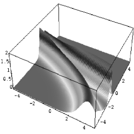
Figure 1: Dynamics of the exact soliton solution of the integrable perturbation of the KdV equation for the field $u(x,t)$. a) 1-soliton with the usual localized form but with an unusual deceleration, reflected in the bending of soliton trajectory in the (x,t)-plane, b) 2-soliton with the usual elastic scattering and phase shift, but with the dynamics dominated by an unusual accelerated motion.

B. Integrable perturbation of the mKdV equation

Integrable equation with a nonholonomic deformation is driven by a perturbing function, which in turn is subjected to a differential constraint. Therefore, analogous to the deformed KdV, constructed above, we can derive a new deformed mKdV equation again from (13), but with reduction $q=r=v$. Interestingly, in this case a single deformation with $n=1,$ corresponding to the constraint (10) is sufficient to produce the lowest perturbation we are interested in, yielding the perturbed mKdV

$$v_{t}-v_{xxx}-6v^{2}v_{x}=w_{x}(t,x),$$ (19)

$$w_{xx}-2v(c^{2}(t)-w_{x}^{2})^{\frac{1}{2}}=0.$$ (20)

To see the effect of deformation more closely we construct explicitly 1- soliton solution, referring to [20] for the details of the the details on the general N-soliton. The accelerating soliton of the perturbed mKdV, shown in Fig. 2, has the explicit form

$$v(x,t)=\frac{v_{0}}{2}{\rm sech}\xi,\ \xi=\kappa(x-vt)+\phi,\ v=v_{0}+v_{d}$$ (21)

where $v_{0}=4\kappa^{2}$ is the usual constant velocity of the mKdV soliton, while $v_{d}=\frac{2\tilde{c}(t)}{v_{0}t}$ is the unusual time-dependent part of the velocity, induced by the deformation. Note that the perturbing function $w(x,t)$ itself takes a self-consistent solitonic form

$$w_{x}=c(t)\kappa{\rm sech}\xi{\rm tanh}\xi$$ (22)

and drives the field soliton (21) to an accelerated motion again through its asymptotic value $w(x,t)|_{|x|\to\infty}=c(t)$, sitting as a forcing term at the space boundaries.

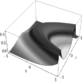
Figure 2: Exact accelerated soliton in the (x,t)-plane for the integrable perturbed mKdV equation.

. C. Integrable perturbation of the NLS equation

For constructing the integrable perturbation of the NLS equation the stage is already set in (9), since with a reduction $r=q^{*}$ and a minimum deformation (10), it would yield the NLS case

$$iq_{t}-q_{xx}-2|q|^{2}q=g,\$$ (23)

with the perturbative function $g(x,t)$ subjected to a nonholonomic differential constraint

$$g_{x}=-2iaq,\ a_{x}=i(qg^{*}-q^{*}g)$$ (24)

where $G^{(1)}_{12}=g,\ G^{(1)}_{21}=g^{*},\ G^{(1)}_{11}=-G^{(1)}_{22}=a$ are the deforming functions coupled through the basic fields $q,q^{*}$ . The set of constraints (24) may be simplified to a single differential constraint

$$\hat{L}(g)\equiv g_{xx}q-g_{x}q_{x}-2q^{2}(qg^{*}-q^{*}g)=0.$$ (25)

Eliminating the deforming function $g$ from (23) and (25) we can further derive a new 4th-order NLS equation expressed through the basic field as

$$(q\partial_{xx}^{2}-q_{x}\partial_{x})(iq_{t}-q_{xx}-2|q|^{2}q)+2q^{2}(i(|q|^{2})_{t}+(qq^{*}_{x}-q^{*}q_{x})_{x})=0.$$ (26)

As already mentioned, this perturbed system can be solved exactly through the ISM. Remarkably however, we can actually avoid the involved procedure of the ISM in all such integrable nonholonomic deformations and can obtain the explicit soliton solutions for these deformed equations by just suitably deforming the known undeformed solutions. As a rule the perturbing affect keeps the form of the soliton intact, while it deforms some parameters like velocity, frequency etc., making them in general time-dependent.

More precisely, in case of the deformed NLS, the original soliton velocity $v_{0}$ and the frequency $\omega_{0}$ of its enveloping wave are changed with an addition of a deformed velocity $v_{d}(t)=\frac{\tilde{c}(t)}{t|\lambda_{1}|^{2}}$ and the deformed wave frequency $\omega_{d}(t)=-2\frac{\tilde{c}(t)\xi}{t|\lambda_{1}|^{2}}$, where $\lambda_{1}=\xi+i\eta$. The function $\tilde{c}(t)$ responsible for such deformation is linked to the asymptotic value of the perturbing function. The accelerating NLS soliton qualitatively looks like that of the mKdV when the dynamics of $|q|$ is plotted (see Fig.2).

We can generate again a two-fold integrable hierarchy for the perturbed NLS system. The first one is the known hierarchy of higher order NLS equations with a perturbation constrained by the same nonholonomic deformation (25), while the second one is a new integrable hierarchy, where the same perturbed NLS equation (23) is perturbed by a hierarchy of higher order deformations of the form (12). For example, the next to the lowest order deformation (25) would include another deforming function $e(x,t)$, in addition to function $g(x,t)$ . Interestingly in this double-deformation the main equation would remain same as the perturbed NLS equation (23), while the constraint equation for $g$ would be changed to

$$\hat{L}(g)+2i(eq_{x}-qe_{x})=0,\$$ (27)

or $$g_{xx}q-g_{x}q_{x}-2q^{2}(qg^{*}-q^{*}g)+2i(eq_{x}-qe_{x})=0,$$

coupling to both the field $q$ and the function $e$. The second deforming function $e$ in turn is constrained exactly by the same differential constraint (25) as

$$\hat{L}(e)=0,\ \ \mbox{or \ \ }e_{xx}q-e_{x}q_{x}-2q^{2}(qe^{*}-q^{*}e)=0.$$ (28)

Even though these new integrable perturbed NLS equations seem to be rather academic, it is intriguing that, a model like our perturbed system (23-25) is implemented already in doped fiber for efficient optical communication and therefore the implementation of the higher order integrable deformation discovered here for a a similar multi-doped system seems to be a promising possibility [21].

D. Integrable perturbation of the SG equation

Notice that in the line of the present approach, the well known SG equation in the light-cone coordinates, which can be obtained through reduction $q=r=\theta_{x}$ from the AKNS system, can itself be considered as a deformation $\theta_{xt}=-i\tilde{g}$ of the linear wave equation $\theta_{xt}=0$, with a constraint (10) on the deforming function $\tilde{g}$. This constraint can be easily resolved as $G^{(1)}_{12}=\tilde{g}=i\sin 2\theta$, yielding the standard SG equation: $\theta_{xt}=\sin 2\theta$ . The situation however becomes more interesting if in the same equation $\theta_{xt}=-i\tilde{g}$, the deformation $\tilde{g}=ig$ is coupled to another deformation $G^{(2)}$ , yielding the nonholonomic constraint (11) in the form

$$g_{x}=-2a\theta_{x}+2e,\ a_{x}=2\theta_{x}g,\ e_{x}=0,$$ (29)

with the matrix elements $G^{(1)}_{11}=a,\ G^{(1)}_{12}=-G^{(1)}_{21}=ig,\ G^{(2)}_{12}=G^{(2)}_{21}=e(t),\ G^{(2)}_{11}=0$, where $e(t)$ is an arbitrary function of $t$ . Expressing (29) through the perturbing function $g$ we obtain the nonholonomic deformation of the SG equation as

$$\theta_{xt}=g,$$ (30)

$$g_{xx}\theta_{x}-g_{x}\theta_{xx}+4g\theta_{x}^{3}+2e(t)\theta_{xx}=0$$ (31)

Note that solving the constraint (29) or equivalently (31) one can get different deformations of the SG equation. We derive one such interesting solution as

$$g = e(t)(\alpha\sin 2\theta+\beta\cos 2\theta),$$

$$a = e(t)(\alpha\cos 2\theta-\beta\sin 2\theta).\ \alpha_{x}=\sin 2\theta,\ \beta_{x}=\cos 2\theta,$$ (32)

which yields a new integrable deformation of the SG as

$$\theta_{xt}=e(t)(\alpha\sin 2\theta+\beta\cos 2\theta),$$ (33)

with $\alpha,\beta$ as defined in (32). It is intriguing to note that, the new SG equation (33) has an additional $\cos 2\theta$ part along with the traditional $\sin 2\theta$ term and the coefficient $e\alpha$, which usually corresponds to the particle mass becomes a space-time dependent function. It is worth mentioning that, though at $e=0$ one can recover from (29) the undeformed standard SG equation, as shown above, we can no longer obtain the standard SG equation from its deformation (33) at $e\to 0$. This new equation (33), which is related to the system considered in [16], should however be examined carefully for the applicability of the ISM. Nevertheless, assuming the existence of its kink solution we present in Fig. 3 the accelerated kink for the field $\theta$ and the soliton solution for the perturbing function for the integrable perturbed SG equation.

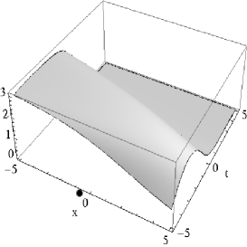
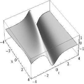
Figure 3: Exact soliton solutions for the integrable perturbation of the sine-Gordon equation. a) Accelerating kink solution for $\theta(x,t)$. b) Perturbation $g(x,t)$ in the solitonic form with nontrivial time-dependent asymptotic $c(t)=0.5t$

.

Continuing the process of higher order differential constraints, by introducing more and more terms with $\lambda^{-n},n=3,4,\ldots$ in $V^{(def)}(\lambda)$, we can generate a hierarchy of integrable higher nonholonomic deformations in most of the cases. In some cases, as the explicit calculations show, one has to add more than one higher terms to get the first nontrivial result.

VI. PRESENT NONLINEARIZATION SCHEME & INTEGRABLE PERTURBATIONS IN THE BACKGROUND OF EARLIER RESULTS

We compared our nonlinearization scheme for generating integrable systems with the AKNS construction in Sec. III.B. It is worth mentioning here that the idea of this nonlinearization bears some analogy as well as differences with the well known Zakharav-Shabat (ZS) dressing method [22]. In the dressing method the Lax pair as well as the soliton solution are constructed starting from the asymptotic vacuum solution. In our nonlinearization scheme on the other hand the Lax operators are build up starting from the linear field equation, based only on the dimensional argument and the notion of the building blocks. In analogy with the ZS dressing method it is however tempting to construct in our scheme the soliton solution for the nonlinear equation starting from the solution of its linearized equation.

Extending our construction further by nonholonomic deformation, we have gone beyond the standard AKNS method and considered perturbing matrices of scaling dimension $L>N$ in the $V_{N}(\lambda)$ operator. This amounts to extending this operator as $V_{N,M}(\lambda)=V_{N}(\lambda)+V_{M}^{(def)}(\lambda)$ by considering, together with the positive powers of $\lambda$ upto $N$, all its negative powers upto $M$. We have shown through such deformations a beautiful universality of the recently found nonholonomic deformation of the KdV system [6, 7], by extending this concept to all members of the AKNS family, including the mKdV, the NLS and the SG equations. At the same time we have discovered a two-fold integrable hierarchy for them, with the explicit finding of some interesting multiple deformation. Our construction allows the application of the exact ISM for obtaining N-soliton solutions for both the field and the perturbing functions, which shows an unusual accelerated motion for the solitons. However a significant advantage of such deformations is that, we can actually avoid the application of the ISM in these cases and construct the exact soliton of the deformed equations by deforming the well known soliton solutions. Such perturbations only deforms the time evolution of the spectral data, which deforms in turn the soliton velocity and for the complex fields also the frequency of the enveloping wave.

It is true that in the long development of the theory of integrable systems, the use of negative powers of $\lambda$ in the Lax operator $V(\lambda)$ was implemented also in few earlier occasions. However a consistent, systematic and full utilization of this procedure including the simultaneous presence of higher positive and negative powers of $\lambda$, associated to all equations in the AKNS family, and most importantly, the possibility of introducing new perturbing functions as multiple deformations, which are our main emphasis here, have never been undertaken. Similarly, the existence of a two-fold integrable hierarchy and exact N-soliton solutions for both the field and the perturbing functions in all integrable perturbed systems of the AKNS family, as well as the possibility of boosting the soliton to accelerated motion by the perturbing function through its time-dependent asymptotic at the space boundaries, as revealed here, were not explored or clarified in any earlier occasions.

As we understand, the AKNS themselves have considered integrable SG and Maxwell-Bloch systems going upto $\lambda^{-1}$ [1]. A -ve hierarchy for the mKdV model was also considered in [16]. However these work either did not consider both +ve and -ve powers of $\lambda$ simultaneously, which would result to the integrable perturbations, or they went away from the perturbative models by considering only the equations for the basic field. Thus these results did not come close to ours, though we can derive them as particular cases of our more general integrable model.

However an important physically applicable model considered earlier [23] can be represented by the lowest order deformation of the NLS equation (23-25) found through our construction. This in turn indicates the physical significance of our integrable perturbed equations and opens up the possibility for application of the hierarchy of perturbed NLS equation, found here, to the nonlinear fiber optics communication through media with multiple doping, by switching to higher order deformations [21].

We should pay special attention to another class of interesting source equations proposed by Melnikov [17] and show that our integrable perturbed models stand as complementary to the Melnikov’s models and can make contact with them at a highly degenerate limit. In the Melnikov’s formalism a set of eigenvalues $\lambda_{n},1,2,\ldots,N$ appear explicitly, which are needed to be distinct and strictly nonvanishing for any construction of those models. However as we show below, our construction could be related in fact to the complementary limit of the Melnikov’s systems, when all these eigenvalues become degenerate and moreover go to zero, simultaneously. Miraculously, Melnikov’s system, in general too complicated, simplifies drastically at this highly degenerate limit and reduces to our simple perturbative model, allowing exact accelerating solitons and suitable for physical applications.

Let us consider as a demonstration Melnikov’s source equation for the NLS system given as

$$iu_{t}+u_{xx}+2|u|^{2}u=\sum_{n}(\phi_{n}^{2}+\psi_{n}^{2})$$ (34)

and its complex conjugate, together with a eigenvalue problem at discrete eigenvalues $\lambda_{n},\ n=1,2,\ldots,N$ for a set of complex functions $(\phi_{n},+\psi_{n})$:

$$\phi_{n,x}+u\psi_{n} = \lambda_{n}\phi_{n}$$

$$\psi_{n,x}+u^{*}\phi_{n} = -\lambda_{n}\psi_{n},$$ (35)

and their complex conjugates. As such this set of $2(1+2N)$ number of coupled complex equations is evidently much more complicated than our perturbed NLS (23-25) and its application to physical models seems to be rather obscure. If however we denote the rhs of (34) by $\sum_{n}(\phi_{n}^{2}+\psi_{n}^{2})=g$ and the combination $\sum_{n}(\phi_{n}\psi_{n}-\phi_{n}^{*}\psi_{n}^{*})=b$, then after some algebraic manipulation from (35) we find

$$g_{x}+2ub = -2\sum_{n}(\lambda_{n}\phi_{n}^{2}-\lambda_{n}^{*}{\psi^{*}_{n}}^{2}),$$

$$b_{x}+ug^{*}-u^{*}g = 0$$ (36)

It is clear that the system closes and immensely simplifies only when all eigenvalues become the same as well as vanishing: $\lambda_{n}=0,n=1,2,\ldots,N$, which however is opposite to the Melnikov’s theory, which strictly demands all $\lambda_{n}\neq 0$. We note immediately that at this vanishing limit from (36) we get

$$g_{x}=-2ub,\ b_{x}=u^{*}g-ug^{*},$$ (37)

which generates our perturbed NLS (23-25) and for the real field reduction $u^{*}=u,\ g^{*}=-g$ reproduce further the perturbed mKdV equation (20). Therefore we may conclude that at highly degenerate limit and in a situation complimentary to the Melnikov’s assumption, the well known source equations reduce to the lowest deformation cases of our perturbed equations. However the possibility of generating higher order deformation for perturbing functions constituting the novel integrable two-fold hierarchy of integrable perturbed equations, we have discovered, seems to be absent in the Melnikov’s formalism.

VII. CONCLUDING REMARKS

The present scheme of nonlinearizing linear equations to integrable systems, though bears similarity with the AKNS approach, differs in its motivation, simplicity and generality. Our procedure does not start from a given integrable nonlinear equation, as customary in the AKNS method, but aims to construct it by nonlinearizing a given linear field equation and is applicable without much difficulty to the AKNS as well as to the KN family. Moreover due to identification of the building blocks of the Lax operators and the effective use of the physical notion of dimensional analysis, our construction of the crucial time-Lax operator $V_{N}(\lambda)$ becomes much simpler. In place of $4(N+1)$ unknown functions, in general complex, in the AKNS scheme obeying coupled partial differential equations, we have only $N+1$ unknown real integers to be determined from simple algebraic equalities. This simplicity of our scheme becomes more evident at higher values of $N$.

The extension of the notion of integrability from the KdV equation to the whole family of the AKNS system was a major breakthrough achieved in early seventies. We now find a similar extension for the nonholonomic deformation of the KdV equation, discovered recently [6, 7], to all members of the AKNS family, which shows the universality of such integrable deformations beyond a single known example [6]. Moreover, by discovering an integrable hierarchy of increasingly higher order deformation for each of these cases, we establish that this universality, in fact is two-fold. One is the known AKNS hierarchy with an additional fixed deformation, while the other is a new integrable hierarchy for each of the NLS, the KdV, the mKdV and the SG equations, deformed by perturbing functions with increasingly higher order nonholonomic constraints. Interestingly, in the second scenario nonlinear integrable equations can be generated by perturbations only, even from a linear dispersionless or trivial equation like $q_{t}=q_{x},\ q_{t}=0$.

Such integrable perturbations are achieved through an extension of our nonlinearization scheme, where we go beyond our building block conjecture and introduce new perturbative functions at every higher step of deformation of the time-Lax operator, making the fullest use of its negative power expansion in the spectral parameter. It seems that, in spite of numerous work in this well studied subject, these two simple steps were not considered earlier consistently, thereby missing a whole class of integrable perturbed equations, which we discover here. These integrable perturbed equations with nonholonomic constraints are different and much simpler than the traditional source equations of Melnikov. Interestingly however, they are related in a exceedingly subtle way, being complementary to each other and linked at a highly degenerate limit. Nevertheless such a relation can be shown to exist only at the lowest order deformation of our equations, while the novel hierarchy of integrable deformation, that we find for our perturbed systems, is totally absent in Melnikov’s source equations.

The nonholonomic deformation inducing new integrable equations presented here are exactly solvable through the inverse scattering method. However an important advantage of such deformed integrable equations is that, one can completely bypass the complicated ISM for extracting their exact soliton solutions and construct them by merely deforming the well known solutions of the unperturbed equations. One finds that under such perturbations the form of the solitons remain the same, while the soliton velocity and the wave frequency get additional terms, capable of introducing acceleration or deceleration in the solitonic motion.

The explicit soliton solutions for the simplest integrable perturbed NLS, mKdV, KdV and SG equations, presented here show such unusual accelerated motion forced by the perturbation. Within this framework of integrable perturbation, one can also arrange these systems to receive consistent multiple forcing, which are expected to have significant physical applications, especially in fiber optics communication in doped media [18, 23, 21].

Extentions of the nonholonomic deformation to the KN family of equations [24] as well as to $2+1$ dimensional models are exciting future problems. Another challenging problem, which we could not solve here, is to construct the soliton solution of the nonlinear equation from the solution of its linearized equation, by using the present nonlinearization scheme, which might define some new dressing method.

References

- [1] M. Ablowitz et al, Stud. Appl. Math. 53, 294 (1974) M. Ablowitz and H. Segur, Solitons and Inverse Scattering Transforms (SIAM, Philadelphia, 1981) S. Novikov et al , Theory of Solitons (Consultants Bureau, NY, 1984)
- [2] Y. Ohta et al, Prog. Theor. Phys. Supl. 94, 210 (1988)
- [3] D. A. Pinotsis, J. Nonlin. Math Phys. 14, 466 (2007)
- [4] M. Lakshmanan and S. Rajasekar, Nonlinear Dynamics (Springer, Heidelberg, 2003)
- [5] D. J. Kaup and A. C. Newell, J. Math. Phys, 19, 798 (1978)
- [6] A. Karsu et al, arXiv: 0708:3247 [nlin.SI] (2007)
- [7] B. A. Kupershmidt, Phys. Lett. A 372, 2634 (2008)
- [8] Y. Yad and Y. Zeng, eprint: arXiv:0810.1986 [nlin.SI] (2008)
- [9] Goldobin et. al., Phys. Rev. Lett. 92, 057005 (2004) ; H. Susanto and S. van Gils, Phys. Rev. B69, 092507 (2004); A. Davidson et. al. Phys. Rev. B 32, 7558 (1985); I. V. Barashenkov, S R Woodford and E V Zemlyanaya Phys. Rev. Lett. 90, 054103 (2003) ; Z. Yan, J. Phys. A 39, L401 (2006) ; N. A. Larkin, Math. Methods Appl. Sc. 29, 751 (2006)
- [10] H. H. Chen and C. S. Liu, Phys. Rev. Lett. 37, 693 (1976);
- [11] M. Salerno, Phys. Rev. A 44, 5292 (1991)
- [12] Anjan Kundu, J. Phys. A 41, 495201 (2008)
- [13] J. A. Gonzales et al, Chaos Solitons & Fractals 28, 804 (2006)
- [14] A. Kundu, J. Math. Phys. 25, 3433 (1984)
- [15] G. L. Lamb Jr., Rev. Mod. Phys. 43, 99 (1971)
- [16] Z. Qiao and W. Strampp, Physica A 313, 365 (2002)
- [17] V. K. Melnikov, Phys. Lett. A 133, 493 (1988) ; V. K. Melnikov, Inverse Problem 6, (1990) 233 (1990); V. K. Melnikov, Inverse Problem 8, 133 (1992) J. Leon, Phys. Lett. A 144, 444 (1990) ; D. J. Zhang,J. B. Bi and H. H. Hao, J. Phys. A 39 , L4627 (2006) ; A. B. Khasanov, G. U. Urazboev, Diff. Eqns. 43, 561 (2007)
- [18] M. Nakazawa, E. Yamada and H. Kubota, Phys. Rev. Lett. 66, 5973 (1991)
- [19] F. Calogero and A. Degasperis, Nuovo Cim. 22, 270 (1978); R. Balakrishnan, A 32, 1144 (1985)
- [20] Anjan Kundu, R. Sahadevan and L. Nalinidevi, J. Phys. A 42, 115213 (2009)
- [21] Anjan Kundu and Porsezian (under investigation)
- [22] V. E. Zakharov and A. B. Shabat, Funct. Anal. & Appl. 8, 226 (1974)
- [23] A. I. Maimistov and E. A. Manyakin, Sov. Phys. JETP 58 (1983) 685; S. Kakei and J Satsuma, J. Phys. Soc. Jpn. 63 (1994) 885
- [24] Anjan Kundu (under preperation), D͡eformation hierarchy of the derivative nonlinear Schrödinger equation and the Lenells-Fokas equation