Half-metallic ferromagnets: From band structure to many-body effects

Abstract

A review of new developments in theoretical and experimental electronic structure investigations of half-metallic ferromagnets (HMF) is presented. Being semiconductors for one spin projection and metals for another ones, these substances are promising magnetic materials for applications in spintronics (i.e., spin-dependent electronics). Classification of HMF by the peculiarities of their electronic structure and chemical bonding is discussed. Effects of electron-magnon interaction in HMF and their manifestations in magnetic, spectral, thermodynamic, and transport properties are considered. Especial attention is paid to appearance of non-quasiparticle states in the energy gap, which provide an instructive example of essentially many-body features in the electronic structure. State-of-art electronic calculations for correlated $d$-systems is discussed, and results for specific HMF (Heusler alloys, zinc-blende structure compounds, CrO${}_{2},$ Fe₃O₄) are reviewed.

I Introduction

Twenty-five years ago the unusual magnetooptical properties of several Heusler alloys motivated the study of their electronic structure. It yielded an unexpected result: some of these alloys showed the properties of metals as well as insulators at the same time in the same material depending on the spin direction. This property was baptized half-metallic magnetism de Groot et al. (1983b). Although it is not exactly clear how many half-metals are known to exist at this moment, half-metallic magnetism as phenomenon has been generally accepted. Formally the expected $100\%$ spin polarization of the charge carriers in a half-metallic ferromagnet (HMF) is a hypothetical situation that can only be approached in the limit of vanishing temperature and neglecting spin-orbital interactions. However, at low temperatures (as compared with the Curie temperature which exceeds 1000K for some HMF’s) and minor spin-orbit interactions a half-metal deviates so markedly from a normal material, that the treatment as a special category of materials is justified. The confusion on the number of well-established half-metals originates from the fact that there is no “smoking gun” experiment to prove or disprove half-metallicity. The most direct measurement is spin-resolved positron annihilation Hanssen and Mijnarends (1986), but this is a tedious, expensive technique requiring very dedicated equipment. The only proven HMF so far is NiMnSb to the precision of the experiment, which was better than one hundredth of an electron Hanssen et al. (1990). This number also sets the scale for concerns of temperature-induced depolarization and spin-orbit effects, detrimental for half-metallicity.

The half-metallicity in a specific compound should not be confused with the ability to pick up $100\%$ polarized electrons from a HMF. The latter process involves electrons crossing a surface or interface into some medium where their degree of spin polarization is analyzed. This is clearly not an intrinsic materials property. The richness but also the complications of surfaces and interfaces are still not fully appreciated.

Because of all these experimental complications, it is not surprising that electronic structure calculations continue to play an important role in the search for new HMF as well as the introduction of new concepts like half-metallic antiferromagnetism. However, electronic structure calculations have weaknesses as well. Most of the calculations are based on density functional theory in the LDA or GGA approximation. It is well known that these methods underestimate the band gap for many semiconductors and insulators, typically by $30\%$. It has been assumed that these problems do not occur in half-metals since their dielectric response is that of a metal. This assumption was disproved recently. A calculation on the HMF La_0.7Sr_0.3MnO₃ employing the GW approximation (that gives a correct description of band gaps in many semi-conductors) leads to a half-metallic band gap 2 eV in excess to the DFT value Kino et al. (2003). The consequences of this result are possibly dramatic: if it were valid in half-metallic magnetism in general, it would imply that many of the materials, showing band gaps in DFT based calculations of insufficient size to encompass the Fermi energy, are actually in reality bona fide half-metals. Clearly much more work is needed in this area.

The strength of a computational approach is that it does not need samples: even nonexistent materials can be calculated! But in such an endeavour a clear goal should be kept in mind. Certainly, computational studies can help in the design of new materials, but the challenge is not so much in finding exotic physics in materials that have no chance of ever being realized. Such studies can serve didactical purposes, in which case they will be included in this review. However, the main attention will be devoted to materials that either exist or are (meta)stable enough to have a fair chance of realization.

This review will cover half-metals and will not discuss the thriving area of magnetic semiconductors. Some overlap exists, however. The much older field of magnetic semiconductors started with semiconductors like the europium monochalcogenides and cadmium-chromium chalcogenides Nagaev (1983). Later, the attention changed to the so-called diluted magnetic semiconductors Delves and Lewis (1963). These are regular (i.e. III-V or II-VI) semiconductors, where magnetism is introduced by partial substitution of the cation by some (magnetic) 3$d$ transition element. The resulting Curie temperatures remained unsatisfactory, however. The next step in the development was the elimination of the non-magnetic transition element altogether. This way HMF’s can be realized provided that the remaining transition-metal pnictides could be stabilized in the zinc-blende or related structures. The review will treat not the (diluted) magnetic semiconductors as such, but some aspects of metastable zinc-blende HMF’s.

HMF’s form a quite diverse collection of materials with very different chemical and physical properties and even the origin of the half-metallicity can be quite distinct. For this reason it is required to discuss the origin of the band gap in terms of two ingredients that define a solid: the crystal structure and the chemical composition. Two aspects are of importance in this context. The first one is “strong magnetism” versus “weak magnetism”. In a strong magnet, the magnetic moment will not increase if the exchange splitting is increased hypothetically. Thus the size of the magnetic moment is not determined by the strength of the exchange interaction, but is limited instead by the availability of electron states. In practice this implies that either the minority spin sub shell(s) responsible for the magnetism is (are) empty or the relevant majority channel(s) is (are) completely filled. In the case of weak magnetism the magnetic moment is determined by a subtle compromise between the energy gain of an increase in magnetic moment (the exchange energy) and the (band) energy the increase of the magnetic moment costs. To avoid misunderstanding, we emphasize that this definition of “weak” and “strong” magnets differs from that used in Moriya’s book Moriya (1985) and most theoretical works on itinerant-electron magnetism. According to Moriya, “strong” magnets are those with well-defined magnetic moments which means, e.g., the Curie-Weiss behavior of the wavevector-dependent magnetic susceptibility $\chi(\mathbf{q},T)$ in the whole Brillouin zone. In this sense, all HMF’s (e.g., containing Mn ions) are strong magnets. However, within this group of materials we may introduce a more fine classification based on the sensitivity of magnetic moment with respect to small variation of parameters.

Any combination of “weak” or “strong” magnetism with majority or minority spin band gaps is known today. Thus ”weak” magnets with minority spin band gaps are found in the Heusler alloys and artificial zinc-blendes, examples of weak magnets with majority spin gaps are the double perovskites and magnetite. The colossal magnetoresistance materials are examples of strongly magnetic half-metals with minority spin band gaps as is for example, chromium dioxide, while the anionogenic ferromagnets like rubidium sesquioxide are examples of a strongly magnetic half-metal with a majority spin band gap.

An interesting and relatively new development is the work on half-metallic sulphides. The HMF state in oxides with the spinel structure is relatively rare. The prime example of course is magnetite. However any substitution into the transition-metal sublattices leads practically invariable to a Mott insulating state, as magnetite itself possesses below the Verwey transition at 120K. On the other hand the electrons in sulphides, are substantially less correlated. Hence a wealth of substitutions is possible in order to optimize properties, design half-metallic ferro- or antiferromagnets etc. without the risk of losing the metallic properties for the second spin direction as well. There is a prize to be paid however: since the cation-cation distances are larger in sulphides, the Curie and Neel temperatures are lower in comparison with the oxides. Nevertheless, the work on half-metallic sulphides deserves strong support.

In all the metallic ferromagnets, interaction between conduction electrons and spin fluctuation is of crucial importance for physical properties. In particular, the scattering of charge carriers by magnetic excitations determines transport properties of itinerant magnets (temperature dependences of resistivity, magnetoresistivity, thermoelectric power, anomalous Hall etc.). From this point of view, HMF, as well as ferromagnetic semiconductors, differ from “normal” metallic ferromagnets by the absence of spin-flip (one-magnon) scattering processes. This difference is also important for magnetic excitations since there no Stoner damping, and spin waves are well defined in the whole Brillouin zone, as well as in magnetic insulators Auslender and Irkhin (1984a); Irkhin and Katsnelson (1994).

Electron-magnon interaction modifies also considerably electron energy spectrum in HMF. These effects take place both in usual ferromagnets and in HMF. However, peculiar band structure of HMF (the energy gap for one spin projection) results in important consequences. In generic itinerant ferromagnets the states near the Fermi level are quasiparticles for both spin projections. On the contrary, in HMF and important role belongs to incoherent (non-quasiparticle, NQP) states which occur near the Fermi level in the energy gap Irkhin and Katsnelson (1994). The appearance of the NQP states in Edwards and Hertz (1973); Irkhin and Katsnelson (1983) is one of the most interesting correlation effects typical for HMF. The origin of these states is connected with “spin-polaron” processes: the spin-down low-energy electron excitations, which are forbidden for HMF in the one-particle picture, turn out to be possible as a superposition of spin-up electron excitations and virtual magnons. The density of the NQP states vanishes at the Fermi level but increases drastically at the energy scale of the order of a characteristic magnon frequency $\overline{\omega}$. These states are important for spin-polarized electron spectroscopy Irkhin and Katsnelson (2001, 2006), NMR Irkhin and Katsnelson (2005a), and subgap transport in ferromagnet-superconductor junctions (Andreev reflection) Tkachov et al. (2001). Recently, the density of NQP states has been calculated from first principles for a prototype HMF, NiMnSb Chioncel et al. (2003a), as well as for other Heusler alloys Chioncel et al. (2006a), zinc-blend structure compounds Chioncel et al. (2005); Chioncel et al. (2006b) and CrO₂ Chioncel et al. (2007). Fig 1 shows in a pictorial way the NQP contribution to the density of states.

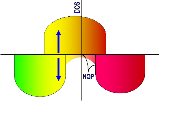
Figure 1: (color online) Density of states of non-quasiparticles, for half-metallic ferromagnets, possessing the gap in the minority spin channel. NQP states are the dominant many-body feature around $E_{F}$ in comparison other mean-field effects, such as spin-orbit or non-collinearity as it will be discussed in the following sections.

Therefore, HMF are very interesting conceptually as a class of materials which may be convenient to treat many-body solid state physics that is essentially beyond band theory. It is accepted that usually many-body effects lead only to renormalization of the quasiparticle parameters in the sense of Landau’s Fermi liquid (FL) theory, the electronic liquid being qualitatively similar to the electron gas (see, e.g., Nozieres (1964)). On the other hand, NQP states in HMF are not described by the FL theory. As an example of highly unusual properties of the NQP states, we mention that they can contribute to the $T$-linear term in the electron heat capacity Irkhin and Katsnelson (1990); Irkhin et al. (1994, 1989), despite their density at $E_{F}$ is zero at temperature $T=0$ K. Some developments concerning physical effects of NQP states in HMF are considered in the present review.

II Classes of half-metallic ferromagnets

II.1 Heusler alloys and zinc-blende structure compounds

In this chapter we will treat HMF with the Heusler C1_b and L2₁ structures. Although being not Heusler alloys in the strict sense, artificial half-metals in the zinc-blende structure will be also discussed because of their close relation with the Heusler C1_b ones. Zinc blende has a face centered cubic (fcc) Bravais lattice with a basis of $(0,0,0)$ and $(1/4,1/4,1/4)$, both species coordinating each other tetrahedrally. The Heusler C1_b structure consists of the zinc-blende structure with an additional occupation of the $(1/2,1/2,1/2)$ site. Atoms at the latter position, as well as those in the origin, are tetrahedrally coordinated by the third constituent, which itself has a cube coordination consisting of two tetrahedra. The Heusler L2₁ structure is obtained by an additional occupation of the $(3/4,3/4,3/4)$ by the same element already present on the $(1/4,1/4,1/4)$ site. This results in occurrence of an inversion center which is not present in the zinc-blende and Heusler C1_b structures. This difference has important consequences for the half-metallic band gaps. Electronic structure of the Heusler alloys has been reviewed recently (from a bit different positions) by Galanakis and Mavropoulos Galanakis and Mavropoulos (2007).

II.1.1 Heusler C1_b alloys

Interest in fast, non-volatile mass storage memory sparked many activities in the area of magnetooptics in general and the magnetooptic Kerr effect specifically in the beginning of the 80-s of last century. All existing magnetic solids were investigated leading to a record MOKE rotation of $1.27^{\circ}$ for PtMnSb van Engen et al. (1983). The origin of these properties remained an unsolved problem. This formed the motivation for the study of the electronic structure of the isoelectronic Heusler C1_b compounds NiMnSb, PdMnSb and PtMnSb and the subsequent discovery of half-metallic magnetism. Interestingly enough, there seems to be still no consensus on the origin of the magnetooptical properties. The original simple and intuitive explanation de Groot (1991) was complementary to the production of spin-polarized electrons by optical excitation in III-V semiconductors. In that case, the top of the valence band is split by the the spin-orbit coupling, and the photoexcitation of electrons from the very top of the band by circularly polarized light leads to 50% spin polarization. Vice versa, excitations from a 100valenceband is possible for only one of the two components of circular light, as in the case of PtMnSb, this should result in a strong difference of refraction and absorption for two opposite polarizations. In PtMnSb this difference is maximal for the visible light, and for NiMnSb the maximum of off-diagonal optical conductivity is shifted to the ultraviolet region. The main contribution to this shift comes from scalar relativistic interactions in the final state Wijngaard et al. (1989), which are much weaker for Ni than for Pt due to difference in nuclear charges. Further the magnetooptical properties of the Heusler alloys were calculated by Antonov et al. Antonov et al. (1997) in a good agreement with experimental data, but the physical explanation was not given in this paper. Recently, Chadov et al Chadov et al. (2006) demonstrated that an agreement between calculated and experimental values of the Kerr rotation and ellipticity in NiMnSb can be further improved by taking into account correlation effects within so-called LDA+DMFT approach (see below Sect.IV.1).

Since NiMnSb is the most studied HMF (at least within the Heusler C1_b’s) we will concentrate on it here. The origin of its half-metallic properties has an analogy with the electronic structure of III-V zinc-blende semiconductors. Given the magnetic moment of $4\mu_{B}$ manganese is trivalent for the minority spin direction, and antimony is pentavalent. The Heusler C1_b structure is the zinc-blende one with an additional site $(1/2,1/2,1/2)$ being occupied. The role of nickel is to supply both Mn and Sb with the essential tetrahedral coordination and to stabilize MnSb in the cubic structure (MnSb in the zinc-blende structure is half-metallic, but not stable). Thus a proper site occupancy is essential: nickel has to occupy the double tetrahedrally coordinated site Helmholdt et al. (1984); Orgassa et al. (1999). The similarity in chemical bonding between NiMnSb and zinc-blende semiconductors also explains why it is a “weak” magnet, in the sense discussed in the Introduction: the presence of occupied manganese minority $d$ states is essential for the band gap. These states play the same role as the metal $p$ states in zinc-blende semiconductors, a situation which is possible only because of the absence of inversion symmetry. The similarity of chemical bonding in Heusler’s and zinc-blende in the original paper de Groot et al. (1983b) was illustrated by ”removing the nickel d states from the Hamiltonian”. This phrasing has lead to considerable confusion. Actually, the coupling of manganese states and antimony states through non-diagonal matrix elements of nickel d states was maintained in this calculation.

Several explanations of the band gap have been given in terms of a Ni-Mn interaction only Galanakis et al. (2002a). While this interaction is certainly present, it is not sufficient to explain the band gap in NiMnSb. These analyses are based on calculations of NiMnSb excluding the antimony, but keeping the volume fixed. This is a highly inflated situation with a volume more than twice the equilibrium one Egorushkin et al. (1983). Under expansion bandwidths in metals decrease, leading eventually to a Mott insulating state. But even before this transition a band gap appear, simply due to the inflation itself. This is not a hypothetical scenario: a solid as simple as elemental lithium becomes a half-metallic ferromagnet under expansion Min et al. (1986), yet there is no evidence for half-metallic magnetism under equilibrium conditions for this element. Also, it is not clear from these considerations why NiMnSb is half-metallic only in the case of tetrahedrally coordinated manganese. Probably the chemical bonding in relation to the band gap is best summarized by in Ref. Kübler (2000): a nickel induced Mn-Sb covalent interaction.

Surfaces of NiMnSb do not show the $100\%$ spin polarization as determined by positron annihilation for the bulk Bona et al. (1985); Soulen et al. (1999). Part of the reason is their tendency of showing surface segregation of manganese Ristoiu et al. (2000). Also, surfaces of NiMnSb are quite reactive and are easily oxidized. But even without contaminations none of the surfaces of NiMnSb are genuinely half-metallic de Wijs and de Groot (2001); Galanakis (2003). This is just another example of the sensitivity of the half-metallic properties in NiMnSb on the correct crystal structure. But this does not necessarily imply that interfaces of NiMnSb with, for example, semiconductors cannot be completely spin-polarized. For example, it was shown that at the $111b$ interface of NiMnSb with CdS or InP the HMF properties are completely conserved, if the semiconductors are anion terminated at the interface de Wijs and de Groot (2001). This anion-antimony bond may look exotic, but such a coordination is quite common in minerals like costobite and paracostobite (minerals are stable on a geological timescale) No experimental verification is at hand at this moment, partially because experimentalists tend to prefer the easier $100$ surfaces in spite of the fact that calculations show that no half-metallic properties are possible here.

Several photoemission measurements have been reported on NiMnSbCorrea et al. (2006) as well as the closely related PtMnSb Kisker et al. (1987). We concentrate on the latter one, because it is the first angular-resolved measurement using single crystalline samples. A very good agreement with the calculated band structure was obtained. This is a remarkable result. In calculations based on density functional theory eigenvalues depend on the occupation. These occupations deviate from the ground state in a photoemission experiment. To very good precision the dependence of the eigenvalues on the occupation numbers is given by the Hubbard parameter $U$. The consequence is that the effective $U~{}$value in alloys like NiMnSb and PtMnSb is much smaller then, e.g., in Ni metal where photoemission experiments indicate the satellite structure related to the so-called Hubbard bands Lichtenstein et al. (2001).

The transport properties of NiMnSb were studied extensively Otto et al. (1989); Hordequin et al. (2000); Borca et al. (2001) (a theoretical discussion of transport properties in HMF is given in Sect. III.9). At low temperatures, the temperature dependence of the resistivity follows a $T^{2}$ law. However, the $T^{2}$ law at low temperatures is absent in thin films Moodera and Mootoo (1994). At around 90K a transition takes place, beyond which the temperature dependence is $T^{1.65}$. The nature of this phase transition is unknown. One possibility is the effect of thermal excitations provided the Fermi energy is positioned close to the top of the valence band or the bottom of the conduction band. For example, in the latter case thermal excitations are possible from the metallic majority spin direction to the empty states in the conduction band of the minority spin direction. Such excitation reduces the magnetic moment, which in its turn will reduce the exchange splitting resulting in an even further reduction of the energy difference between Fermi energy and bottom of the conduction band. This positive feed-back will lead to a collapse of the half-metallic properties at a certain temperature. An analogous situation exists for $E_{F}$ close to the valence band maximum. Numerical simulations indicate that this scenario is highly unlikely in the case of NiMnSb because of its unusual low density of states at the Fermi energy. Another explanation has been put forward based on the crossing of a magnon and a phonon branch at an energy corresponding to 80K Hordequin et al. (1997a, b). It is unclear how this phonon-magnon interaction influences the electronic properties of NiMnSb.

Local magnetic moments were studied experimentally as a function of temperature with polarized neutron scattering. The manganese moment decreases slightly with temperature from 3.79 $\mu_{B}$ at 15K to 3.55 $\mu_{B}$ at 260K, while the nickel moment remains constant at 0.19 $\mu_{B}$ in the same temperature range. On the other hand, magnetic circular dichroism shows a reduction of both the manganese and nickel moments around 80K. Borca et al. Borca et al. (2001) conclude that at the phase transition the coupling of the manganese and nickel moments is lost. A computational study Lezaic et al. (2006) shows vanishing of the moment of nickel at the transition temperature. None of these anomalies are reflected in the spontaneous magnetization Otto et al. (1989) of bulk NiMnSb.

Two Heusler C1_b alloys exist, isoelectronic with NiMnSb: PdMnSb and PtMnSb. Their electronic structures are very similar, but we will discuss the differences. The calculated DFT band structure for PdMnSb is not half-metallic. The minority spin direction does show a band gap very similar as NiMnSb but the Fermi energy intersects the top of the valence band. Reliable calculations (e.g., based on the GW approximation) are needed here to settle the issue whether PdMnSb is half-metallic or not. PtMnSb is very similar to NiMnSb, the largest differences being in the empty states just above the Fermi energy. The direct band gap (at the gamma point) is between the triplet top of the valence band (neglecting spin-orbit interactions) and a total symmetrical singlet state in PtMnSb. This singlet state is positioned at much higher energy in NiMnSb. These differences have been attributed to the much stronger mass-velocity and Darwin terms in platinum Wijngaard et al. (1989). Platinum does not carry a magnetic moment in PtMnSb. Consequently, no 90K anomaly like in NiMnSb is to be expected and none has been reported so far.

Let us consider whether half-metals in the Heusler C1_b structure exist when substituting other than iso-electronic elements for Ni in NiMnSb. Since NiMnSb is a weak magnet, substitutions with elements reducing the total magnetic moment are possible only while maintaining the half-metallic properties. Thus cobalt, iron manganese and chromium will be considered. The case of Co was studied by Kübler Kübler (1984). The half-metallic properties are conserved, consequently the magnetic moment is reduced to $3\mu_{B}$. Calculations on FeMnSb de Groot et al. (1986), MnMnSb Wijngaard et al. (1992) as well as CrMnSb de Groot (1991) all show the preservation of the half-metallic properties. In the case of FeMnSb this implies a reduction of the total magnetic moment per formula unit to $2\mu_{B}$, which is an unusually small moment to be shared by iron and manganese. The way out is that FeMnSb orders antiferromagnetically. Thus the $2\mu_{B}$ total magnetic moment corresponds to the difference in moments of iron and manganese rather than to their sum implied by ferromagnetic ordering. This way to preserve a band gap (energetically favorable from a chemical-bonding point of view) together with the maintenance of sizable magnetic moments (favorable for the exchange energy) determine the magnetic ordering here. Both these effects are usually larger than the exchange-coupling energies. The antiferromagnetic ordering is maintained in MnMnSb with a total moment of $1\mu_{B}$. In the case of CrMnSb the antiferromagnetic coupling leads to a half-metallic solution with a zero net moment. This is a really exotic state of matter. It is genuinely half-metallic, implying $100\%$ spin polarization of the conduction-electrons, yet it lacks a net magnetization de Groot (1991). The stability of such a solution depends sensitively on the balance between the energy gain of the band gap and the energy gain due to the existence of magnetic moments: if the first one dominates a nonmagnetic semiconducting solution will be more stable (remember that both spin directions are isoelectronic here).

In reality, the situation is more complex. CoMnSb does exist, but it crystallizes in a tetragonal superstructure with Co partially occupying the empty sites Senateur et al. (1972). The magnetic moments deviate from the ones expected for a half-metallic solution. FeMnSb does not exist, but part of the nickel can be substituted by iron. Up to 10$\%$ the Heusler C1_b structure is maintained, from 75$\%$ to 95$\%$ a structure comparable with CoMnSb is stable and between 10$\%$ and 95$\%$ both phases coexist de Groot et al. (1986). MnMnSb exists, orders antiferromagnetically and has a net moment of 1$\mu_{B}$. It does not crystallize in the Heusler C1_b structure and consequently is not half-metallic. CrMnSb exists, is antiferromagnetic at low temperatures, and shows a transition at room temperature to a ferromagnetic phase.

A different substitution is the replacement of Mn by another transition metal. An interesting substitution is a rare earth element R. Because of the analogy of half-metals with C1_b structure and III-V semiconductors one expects NiRSb compounds to be nonmagnetic semiconductors.

Several of these compounds do exist in the C1_b structure, examples are Sc, Y and heavy rare-earth elements from the second half of the lanthanide series. All of them are semiconductors indeed Pierre et al. (1999); Pierre and Karla (2000). Doping of NiMnSb by rare earth elements has been suggested as a way to improve the finite-temperature spin polarization in NiMnSb. These substitutions do not influence the electronic band structure much, (see also Sect. V.1.2), the band gap for the minority spin direction remaining completely intact. However, the random substitution of nonmagnetic (Y, Sc) or very different (Ho-Lu) magnetic elements for manganese will modify the magnon spectrum Attema et al. (2004); Chioncel (2004). This could be beneficial to increase spin polarization in some temperature range.

II.1.2 Half-metals with zinc-blende structure

The Curie temperatures of diluted magnetic semiconductors remain somewhat disappointing. A solution is to replace all the main group metals by transition metals. But there is a heavy prize to be paid: These systems can only be prepared as metastable states – if at all – on a suitable chosen substrate. An alternative to come to the same conclusion is to consider Heusler C1_b’s with larger band gaps. This is most easily accomplished by replacement of the antimony by arsenic or phosphorous. No stable Heusler C1_b alloys exist with these lighter pnictides, however. An alternative is to try to grow them as metastable systems on a suitable chosen substrate. This makes the nickel superfluous: since it fails in the case of lighter pnictides to play the role it does so well in the NiMnSb. The bottleneck in this quest is not so much in predicting systems that are good half-metals, but to design combinations of half-metals and substrates that are meta-stable enough to have a chance of being realized experimentally.

Shirai et al. Shirai et al. (1998) were the first to relate concentrated magnetic semiconductor with half-metallic magnets in their study of MnAs in the zinc-blende structure. The experimental realization showed an increase of the Curie temperature indeed: 400K was reported on for CrAs grown on GaAs. Xie et al. Xie et al. (2003b) calculated the stability of all 3$d$ transition-metal chalcogenides in the zinc-blende with respect to the ground state structure. Chromium telluride and selenide, as well as vanadium telluride, are good half-metals which are stable towards a tetrahedral and rhombohedral distortions. Zhao and Zunger Zhao and Zunger (2005) consider the stability of an epitaxial layer as a function of the lattice parameter of the substrate allowing for relaxation in the growth direction. The result is that while the bulk zinc-blende phase is always unstable with respect to the (equilibrium) NiAs structure, there exist lattice constants where the epitaxial zinc-blende phase is more stable as compared with the epitaxial nickel arsenide structure. This is realized (computationally) for half-metallic CrSe.

An alternative to the concentrated III-V magnetic semiconductors is given by delta doped III-V semiconductors. Here the magnetic properties are not introduced by a more or less homogeneous replacement of main group metals by magnetic transition metals. Instead, a very thin transition-metal layer is sandwiched between undoped III-V semiconductor material Nazmul et al. (2002). A clear increase in Curie temperature results Chiba et al. (2003). This is not unrelated to the interface-half-metallicty introduced before de Groot (1991).

II.1.3 Heusler L2₁ alloys

The crystal structure of the Heusler L2₁ alloys is closely related with that of the C1_b alloys. In the L2₁ structure the $(1/2,1/2,1/2)$ position, empty in the C1_b structure, is occupied by the same element that occupies the $(0,0,0)$ position. The similarity in structure suggests a similarity in interactions and physical properties, but on the contrary, the interactions and the physical properties of the two classes are actually quite distinct. The introduction of the fourth atom in the unit cell introduces an inversion centre in the crystal structure. The bandgap in the C1_b compounds resulted from an interaction very similar to that in III-V semiconductors, where the manganese $t_{2g}$ $d$ electrons play the role of the $p$ electrons in the III-V semiconductor. This is no longer possible in the presence of an inversion centre. Consequently bandwidths are reduced and usually Van Hove singularities occur in the vicinity of the Fermi energy. The smaller bandwidth leads to several (pseudo) gaps. Correlation effects are expected to become better observable here.

Another difference is the occurrence of defects. Experimentally it was noted that “The strong effect of cold work on Heusler alloys (L2₁ structure) contrasts with almost unobservable effects in the C1_b structure alloy NiMnSb” Schaf et al. (1983). But also here there are indications that defects that destroy the bandgap are energetically less favourable.

Experimental work goes back to Heuβler in the beginning of the last century. The motivation of his work was the possibility of preparing magnetic alloys out of non-magnetic elements Heusler (1903) (A material was only considered magnetic in that period if it possessed a spontaneous net magnetisation). More recently the landmark work of Ziebeck and Webster on neutron-diffractions investigations Ziebeck and Webster (1974) deserves mentioning as well as the NMR work in the Orsay group of Campbell.

The first bandstructure calculations were by Ishida and coworkers Ishida et al. (1976b, a); Ishida et al. (1980, 1982), as well as Kuebler, Williams and Sommers Kübler et al. (1983). The latter paper contains a clue to half-metallic properties in the L2₁ compounds: the authors remark that “The minority state densities at the Fermi energy for ferromagnetic Co₂MnAl and Co₂MnSn nearly vanish. This should lead to peculiar transport properties in these two Heusler alloys”.

Calculations that explicitly addressed the question of half-metallic properties in the full heuslers appeared not earlier than in 1995 Fujii et al. (1995); Ishida et al. (1995). A systematic study of the electronic structure of Heusler L2₁ compounds was undertaken by Galanakis, Dederichs and Papanikolaou Galanakis et al. (2002b). This paper also reviews the work on half-metallic magnetism in full heusler compounds till 2002. For this reason we refer to it for details and concentrate on subsequent developments here.

The heusler L2₁ compounds take a unique position in the spectrum of halfmetals because of their Curie temperatures. High Curie temperatures are important in the application of halfmetals at finite temperature, since many of the depolarisation mechanisms scale with the reduced temperature $T/T_{c}$. Curie temperatures approach 1000K: Co₂MnSn shows a Curie temperature of 829K, the Germanium analogue 905K while Co₂MnSi was a record holder for some time with a Curie temperature of 985K Brown et al. (2000). A further increase was realized in Co₂FeSi. Experimentally it shows an integer magnetic moment of 6 $\mu_{B}$ and a Curie temperature of 1100K Wurmehl et al. (2005). This result was not reproduced in calculations employing the LDA approximation. The magnetic moment of 6 Bohr-magnetons could only be reproduced by the application of U in excess of 7.5 electron-volt. This is an unusual high number and alternative explanations should also be considered. The question of lattice defects has been studied. On the basis of neutron-diffraction, Co-Fe disorder could be excluded, but no data are available for the degree of Fe-Si interchange. A calculation of the magnetic saturation moment as function of the iron-silicon disorder seems a logical next step in the understanding of this fascinating compound.

Whereas the investigations of the bulk electronic structures of full heuslers has advanced comparable as with the half-heuslers, the situation with respect of the preservation of halfmetallic properties at surfaces and interfaces clearly still lacks behind. Two important results were obtained recently. One result is the preservation of halfmetallic properties of an Co₂MnSi (001) surface provided it is purely manganese terminated. This is the only surface of this half-metal showing this property Hashemifar et al. (2005).

No genuine halfmetallic interfaces between full-heuslers and semiconductors are reported yet. But the results for Co₂CrAl/GaAs look promising. For an (110) interface a spin-polarization of $\approx 90\%$ was obtained Nagao et al. (2004). Although this is clearly not a genuine half-metallic interface yet it should provide a good basis for analyses why half-metallic behaviour is lost at in interface in analogy with the successful work for the C1_b case.

An interesting development in half-metallic-magnetism is in electron-deficient full-Heusler alloys. Reduction of the number of valence electrons to 24 per formula unit leads to either a non-magnetic semiconductor or a halfmetallic anti-ferromagnet. But remarkable enough, the reduction or the number of valence-electrons can be continued here, re-entering a range of half-metals but with a bandgap for the majority spin-direction now. This is best exemplified for the case of Mn₂VAl. It is a halfmetallic ferrimagnet of calculated with the generalized gradient exchange-correlation potential Weht and Pickett (1999). Halfmetals with a bandgap for the majority spin-direction hardly occur. The search for new candidates should strongly be supported.

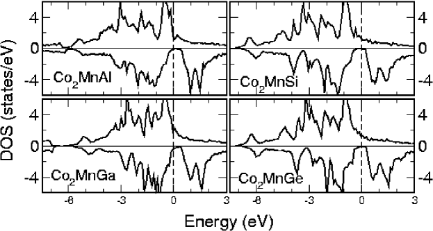
Figure 2: Atom-resolved DOS for the Co₂MnZ compounds with Z=Al, Si, Ge, Sn Galanakis et al. (2006).

II.2 Strongly magnetic half-metals with minority spin gap

II.2.1 Chromium dioxide

Chromium dioxide is the only metallic oxide of chromium. It orders ferromagnetically with a Curie temperature of about 390 K. Its half-metallic state was discovered by band structure calculations Schwarz (1986); Matar et al. (1992). The origin of the half-metallicity is straightforward: in an ionic picture the chromium is in the form of a Cr⁴⁺ ion. The two remaining $d~{}$electrons occupy the majority $d~{}$states. The crystal field splitting is that of a (slightly) deformed octahedron. The valence band for the majority-spin direction is 2/3 filled, hence the metallic properties. The minority-spin $d$ states are at a significant higher energy due to the exchange splitting. For this reason the Fermi level falls in a band gap between the (filled) oxygen 2$p$ states and the (empty) chromium $d$ states. Thus the HMF properties of chromium dioxide are basically a property of chromium and its valence and, as long as the crystal-field splitting is not changed too drastically, the half-metallic properties are conserved. This implies that the influence of impurities should not be dramatic and a number of surfaces retain the half-metallicity of the bulk. As a matter of fact, all the surfaces of low index are half-metallic with a possible exception of one of the (101) surfaces van Leuken and de Groot (1995); Attema et al. (2006). Although initial measurements did not confirm these expectations Kämper et al. (1987), they were confirmed later by the experiments like tunneling Bratkovsky (1997), Andreev reflection Ji et al. (2001) on well-characterized surfaces. Recently, the flow of a triplet-spin supercurrent has been realized in CrO₂ sandwiched employing two superconducting contacts Keizer et al. (2006).

As mentioned before, an interesting question is the origin of the metallic ferromagnetism in CrO₂. This was explained in terms of the double exchange (Zener) model by Korotin et al. Korotin et al. (1998); Schlottmann (2003). The octahedral coordination in the rutile structure is slightly distorted. This leads to splitting of the degenerate $t_{2g}$ state into a more localized $d_{xy}$ state and more delocalized $d_{xz}$ and $d_{yz}$ states (or linear combinations of these). The localized filled $d_{xy}$ state plays the same role as the filled $t_{2g}$ majority spin state in the Zener double-exchange model, while the partially occupied $d_{xy}\pm d_{yz}$ majority states in CrO₂ the role of the partially occupied $e_{g}$ states. The transport properties of CrO₂ were investigated in detail Watts et al. (2000) and interpreted in terms of a two-band model, very much in line with the double exchange model for CrO₂.

The importance of explicit electron-electron interactions in CrO₂ remains a subject of active research. On one hand, Mazin, Singh and Ambrosch-Draxl Mazin et al. (1999) compared LSDA calculations with experimental optical conductivities and found no indications for strong correlations related exotic phenomena. On the other hand, Craco, Laad and Müller-Hartman Craco et al. (2003); Laad et al. (2001) considered photoemission results and conductivity (both DC and optical) and concluded the importance of dynamical correlation effects. The ferromagnetic correlated state was investigated also in a combined local and non-local approach Chioncel et al. (2007) which demonstrates that the $d_{xy}$ orbital is not completely filled and localized as described by LDA+U or model calculations Korotin et al. (1998); Schlottmann (2003); Toropova et al. (2005). More recently, Toropova, Kotliar, Savrasov and Oudovenko Toropova et al. (2005) concluded that the low-temperature experimental data are best fitted without taking into account the Hubbard $U$ corrections. Chromium dioxide will clearly remain an area of active research.

II.2.2 The colossal magnetoresistance materials

The interest in ternary oxides of manganese with di- or trivalent main group metals goes back to Van Santen and Jonker Jonker and Santen (1950). The occurrence of ferromagnetism in transition metal oxides, being considered unusual at that time, was explained by Zener Zener (1951) by the introduction of “double exchange” mechanism. In 70th and 80th these systems were investigated theoretically in connection with the problem of phase separation and “ferron” (magnetic polaron) formation in ferromagnetic semiconductors Auslender and Katsnelson (1982); Nagaev (1983). The interest in spintronics fifteen years ago revived the interest in the ternary manganese perovskites, generally referred to as colossal magnetoresistance materials. A wealth of interesting physics is combined in a single phase diagram of, for example, La_1-xSr_xMnO₃. From a “traditional” antiferromagnetic insulator for $x=1$, the reduction of $x$ results in a ferromagnetic metallic state, while finally at $x=0$ a Mott insulating antiferromagnet is found. Some of the transitions are accompanied with charge and or orbital ordering. Finite temperatures and applied magnetic fields complicate the phase diagram substantially. The ferromagnetic metallic phase for intermediate values of $x$ is presumably half-metallic Pickett and Singh (1996). We will concentrate on this phase here and refer to other reviews for a more complete overview of the manganites Salamon and Jaime (2001); Nagaev (2001); Ziese (2002); Dagotto (2003).

Once the occurrence of a ferromagnetic magnetic ordering is explained, the occurrence of half-metallic magnetism is rather straightforward. Manganese possesses around $3.5$ $d$ electrons in the metallic high-spin state; its rather localized majority spin $t_{2g}$ state is filled, the majority, much more dispersive, $e_{g}$ state is partially occupied and the minority $d$ states are positioned at higher energy, thus being empty. Hence a rather large band gap exists for the minority spin at the Fermi energy and the manganites are strong magnets. Correlation effects are expected to be much stronger here. Notice that no reference has been made to the actual crystal structure: subtleties like in the Heusler structure are absent here. The half-metallic properties are basically a property of the valence of the manganese alone. Surface sensitivity of the HMF properties is not to be expected as long as the valence of the manganese is maintained: This is easily accomplished in the layered manganites de Boer and Groot (1999).

Experimental verification of the half-metallic properties has not been without debate. The origin of the controversy is that the calculated position of the Fermi energy in the energy gap is invariably very close to the bottom of the conduction band. The experimental conformation of the HMF behavior by photoemission Park et al. (1998), was contested on the basis of Andreev reflection measurements, that did show minority-spin $d$ states at the Fermi energy Nadgorny et al. (2001); Nadgorny (2007). Also, tunnelling experiments initially casted doubt on the half-metallic properties Jo et al. (2000a, b); Viret et al. (1997). Mazin subsequently introduced the concept of transport half-metal: the Fermi energy may straddle the bottom of the minority spin $t_{2g}$ band, but since these states are localized this does not influence the half-metallic properties, as far as transport is concerned Mazin et al. (1999); Nadgorny (2007). Recent magnetotransport measurements on better samples support the HMF picture of the CMR materials Bowen et al. (2003). The recent GW calculations by Kino et al. Kino et al. (2003) shed a different light on this matter. In these calculations the half-metallic band gap is increased by as much as 2 eV with respect to the DFT value. This implies that the minority spin $d~{}$band is not even close to the Fermi energy and the CMR materials should be considered as genuine, real HMF’s.

II.3 Weakly magnetic half-metals with majority spin gap

II.3.1 The double perovskites

The double perovskites have a unit cell twice the size of the regular perovskite structure. The two transition-metal sites are occupied by different elements. Double perovskites are interesting for two reasons. Half-metallic antiferromagnetism has been predicted to occur for La₂VMnO₆ Pickett (1998) (we will return to this question later in Sect.II.5.2). The second reason the double perovskites are important is that the high Curie temperatures can be obtained in them as compared with the regular perovskites. Sr₂FeMoO₆ was the first example to be studied in this respect by means of band structure calculations Kobayashi et al. (1998). The density of states is shown in figure 3. In the majority spin direction the valence band consists of filled oxygen 2$s$ and 2$p$ states, as well as a completely filled Fe 3$d$ band, showing the usual crystal field splitting. A band gap separates the conduction band, which is primarily formed by molybdenum $d$ states. The minority spin direction shows an occupied oxygen derived valence band and a hybridized $d$ band of mixed iron and molybdenum character. It intersects the Fermi energy.

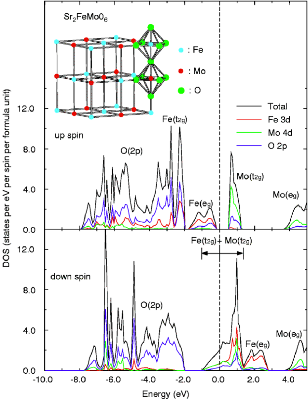
Figure 3: The density of states (DOS) of Sr₂FeMoO₆ Kobayashi et al. (1998)

The Curie temperature is in the range of 410 to 450K. More recently, a similar behavior was found for Sr₂FeReO₆ Kobayashi et al. (1999). Optical measurements did show excitations across the half-metallic band gap of 0.5 eV Tomioka et al. (2000) . A substantial higher Curie temperature is found in Sr₂CrReO₅, $T_{C}=635$K Kato et al. (2002), but band structure calculations show that the band gap for the majority spin direction is closed by the spin-orbit interaction Vaitheeswaran et al. (2005).

II.3.2 Magnetite

Magnetite Fe₃O${}_{4}~{}$ is one of most wide-spread natural iron compounds and the most ancient magnetic material known to humanity. Surprisingly, we still have no complete explanation of its magnetic, electronic and even structural properties, many issues about this substance remaining controversial. At room temperature magnetite has inverted cubic spinel structure with tetrahedral A-sites occupied by Fe³⁺ ions, whereas octahedral B-sites are randomly occupied by Fe²⁺ and Fe³⁺ ions with equal concentrations. Fe₃O₄ is a ferrimagnet with a high Curie temperature $T_{C}\simeq 860$ K. As discovered by Verwey Verwey (1939), at $T_{V}\simeq 120$ K magnetite undergoes a structural distortion and metal-insulator transition. Usually the Verwey transition is treated as a charge ordering of Fe²⁺ and Fe³⁺ states in octahedral sites (for a review, see Mott (1974, 1980)). The nature of the Verwey transition and low-temperature phase of Fe₃O₄ is a subject of numerous investigations which are beyond our topic, see, e.g., recent reviews Walz (2002); Garsia and Sabias (2004). As demonstrated by the band-structure calculation Yanase and Siratori (1984), magnetite in the cubic spinel structure is a rather rare example of HMF with majority-spin gap. This means a saturated state of itinerant $\mathit{3}$d electrons propagating over B-sites, the magnetic moment being close to 4$\mu_{B}$ per formula unit. Recently this picture was questioned by the x-ray magnetic circular dichroism (XMCD) data Huang et al. (2004) which were interpreted as an evidence of large orbital contribution to the magnetization and non-saturated spin state. However, later XMCD experiments Goering et al. (2006) confirm the purely spin saturated magnetic state. Direct measurements of spin polarization by spin-polarized photoemission spectroscopy Mortonx et al. (2002) yield the value about $-40$% (instead of $-100$% predicted by naive band picture), which can be due to both surface effects and electron correlations in the bulk (see Sect.III.3). Transport properties of Fe₃O₄-based films are now intensively studied (see, e.g., Refs. Zhao et al. (2005); Eerenstein et al. (2002)). In particular, a large magnetoresistance owing to electron propagation through antiphase boundaries was found Eerenstein et al. (2002).

Unlike the Heusler alloys, magnetite is a system with a narrow 3d band and therefore strong correlation effects. The fact of the metal-insulator transition itself can be already considered as an evidence of strong electron-electron interaction Mott (1974). The influence of these effects on the electronic structure of Fe₃O₄ has been recently considered in Refs. Craco et al. (2006); Leonov et al. (2006).

II.4 Strongly magnetic half-metals with majority spin gap

II.4.1 Anionogenic ferromagnets

Until recently, strongly magnetic HMF with a majority spin band gap were absent. The chemical composition of the compounds calculated to be half-metallic in this category was quite unexpected: heavy alkali oxides Attema et al. (2005). The magnetic moment is carried by complex oxygen ions, hence the above name. Besides the oxygen molecule, that has two unpaired electrons, the O^2- ion occurs in the so-called hyperoxides like RbO₂ and CsO₂. These are antiferromagnetic insulators with rather low Neel temperatures. Another molecular ion of interest is the non-magnetic peroxide ion O${}_{2}^{2-}$. In the series molecular oxygen – hyperoxide ion – peroxide ion the antibonding $\pi$ orbital is progressively filled, leading to the vanishing of the magnetic moment for the peroxides. Also sesquioxides exist which have composition between peroxide and hyperoxide. They are rather thermally stable, but do react with atmospheric water and carbondioxide. The analogy between the holes in the antibonding double-degenerate $\pi$ level and the electrons in the double-degenerate antibonding $e_{g}$ level of the colossal magnetoresistance materials motivated a computational study. This yielded a HMF state with surprisingly high Curie temperatures (300K). Partial explanation is the absence of superexchange in these oxides, since the mediator for it, the alkali ions, do not possess the required electron states in the vicinity of the Fermi level. Direct experimental evidences are unfortunately lacking. An indirect evidence is the cubic crystal structure measured down to 5K (unlike peroxides and hyperoxides), the crystallographic equivalence of the molecular oxygen ions, the occurrence of charge fluctuations down to 5K Jansen et al. (1999), the opaque optical properties and indications of unusual widths of the stability regions of the sequioxides in the oxygen-rubidium and oxygen-caesium phase diagrams Rengade (1907).

II.5 Sulphides

The spectacular developments in the area of high temperature superconductivity succeeded by the interest in colossal magnetoresistance materials have pushed the interest in sulphides and selenides somewhat to the background. These materials have some advantages over oxides, however. Two main differences, both due to the increased metal-anion covalence as compared with oxides, are of importance here: the more correlated behavior of the oxides as well as their preference for a high-spin configuration. Sulphides often prefer a low-spin configuration, which make their behavior less predictable without careful computation. So, the sulphur analogue of magnetite, the mineral Greigite, has a magnetic moment of $2\mu_{B}$ only, compared with the $4\mu_{B}$ of magnetite. Consequently, it is not half-metallic. In the widespread mineral pyrite FeS₂, iron has a non-magnetic $d^{6}$ configuration, unimaginable in oxides. As mentioned before, magnetite shows half-metallic properties, but is at the brink of Mott localization: cooling down below 120K suffices to accomplish this. On the other hand, the much less correlated behavior of sulphospinels allows the occupation of a broad range of different transition metals on the octahedral and tetrahedral cation sites without the risk of a Mott insulating state. This does not hold for all the pyrites, however. Thus FeS₂ is a non-magnetic semiconductor. The excellent agreement between LDA calculations and the photoemission spectra indicate negligible correlation effects Folkerts et al. (1987). CoS₂ is a ferromagnetic metal with a Curie temperature of 122K. The magnetic moments were calculated function of the Hubbard U and comparison with experimental data indicated the importance of $U$ (of less than 1 eV). NiS₂ is a Mott insulator. NiSe₂ is metallic while in NiSe_2xS_2(1-x) the strength of the correlation effects can be adjusted by variations in the composition.

Magnetic ordering temperatures, important for maintaining the polarization of charge carriers at finite temperature, of oxides are usually superior to those of sulphides and selenides.

II.5.1 Pyrites

Saturated itinerant ferromagnetism in the pyrite-structure system Fe_1-xCo_xS₂ was discovered experimentally in Ref. Jarrett et al. (1968) and discussed from the theoretical-model point of view in Ref. Auslender et al. (1988). Half-metallic ferromagnetism in pyrites was first considered in band calculations by Zhao, Callaway and Hayashibaran Zhao et al. (1993). Their results for CoS₂ show near the Fermi energy two completely filled $t_{2g}$ bands for the two spin directions, a partial filled $e_{g}$ majority band as well as a minority $e_{g}$ band just overlapping the Fermi energy. At slightly higher energy the antibonding sulphur 3$p$ states are found. Clearly, cobalt disulphide is an almost half-metallic ferromagnet. Also it is suggested that half-metallic magnetism can be obtained in the ternary system Fe_xCo_1-xS₂, an idea further worked out by Mazin Mazin (2000). He calculated the expected HMF region in the phase diagram to extend from $0.2$ to $0.9$. A detailed study, both computational and experimental Wang et al. (2005), reveals a strong dependence of the spin polarization at the Fermi level on the composition. Theoretically, $100\%$ spin polarization is obtained for $x=0.25$, whereas the maximal polarization ($85\%$) determined with Andreev reflection at 4.2K is obtained at $x=0.15$. The polarization drops for higher concentrations of iron. The Fermi level is located very close to the bottom of the conduction band. This can lead to thermal instabilities of the half-metallicity as discussed for NiMnSb. Recently half-metallic properties of pyrite-structure compounds have been reviewed by Leighton et. al. Leighton et al. (2007).

II.5.2 Spinels

The activities in the area of half-metallicity are somewhat underrepresented. A complication in this class of compounds is that of cation ordering. The application of high temperatures leads to disproportionation, so long annealing at lower temperatures may be required. The type of cation ordering depends on the preparation conditions. On the other hand, once being controlled, the cation occupancy can form a degree of freedom to achieve HMF materials.

One of the compounds considered in a study on chromium chalcogenides is of interest here CuCr₂S₄. It shows an almost HMF band structure: the Fermi level is positioned 50 meV below the top of the valence band Antonov et al. (1999).

Sulphospinels were also considered in detail in the quest for the elusive half-metallic antiferromagnet Park et al. (2001); Min et al. (2004). Mn(CrV)S₄, with chromium and vanadium occupying the octahedral sites is calculated to fulfill all the requirements. It shows a band gap of approximately 2eV, while the Fermi level intersects a band of primarily vanadium character. The Mn moment is compensated by the moments of chromium and vanadium on the octahedral sites. Another sulphospinel with predicted half-metallic properties is (Fe_0.5Cu_0.5)(V_0.5Ti_1.5)₂S₄. In this case, the metallic behavior is attributed to the atoms at the tetrahedral site; their magnetic moments are exactly canceled by those at the octahedral site.

II.6 Miscellaneous

II.6.1 Ruthenates

The 3$d$ transition-elements and their compounds have been studied in much more detail as compared with their 4$d$ and 5$d$ analogues. Part of the reason is that magnetism is expected to be favored more in the 3$d$ series where no d core is present. Ruthenium is a perfect example of the contrary. The binary and ternary oxides of this 4d transition metal show a rich variety of physical properties like ferromagnetism in SrRuO₃, unconventional superconductivity in Sr₂RuO₄ Maeno et al. (1994). Here we consider the case of SrRuO₃. Ruthenium is tetravalent in this compound, just as in RuO₂. The latter compound is a non-magnetic metal with 4$d$ electrons in the slightly split $t_{2g}$ subband. In SrRuO₃, a magnetic, low-spin state occurs with a filled $t_{2g}$ majority spin band and a partially filled $t_{2g}$ minority spin band. Thus all the ingredients seem to be present for a half-metal. Calculations show that the exchange and crystal field splitting is not sufficient to create a band gap large enough to encompass the Fermi energy. Recently, it was shown that the application of the LDA+U method leads to a substantial increase in band gap in conjunction with orbital ordering. Thus a half-metallic solution is obtained. Comparison with experiment does not lead to a definite conclusion. No experimental determination of $U$ is available. The measured magnetic moment is more in line with the LDA results ($0.8\div 1.6$ $\mu_{B}$), but extrapolation to the high-field limit could lead to an integer magnetic moment. There is no experimental evidence for orbital ordering, however.

The research on ruthenates is relatively recent and especially ternary compounds have not yet been investigated exhaustively.

II.6.2 Organic half-metals

Conducting organic materials have been an area of active research since the discovery of electrical conduction in doped polyacethylene Shirakawa et al. (1977). A surge of activities has resulted in applications generally referred to as plastic electronics. Recently, attempts have started to develop HMF suitable for these applications. Originally, the focus was on carbon nanotubes where magnetism was achieved by the introduction of 3d metals. Calculations were performed for 3,3 single wall carbon nanotubes with a linear iron nanowire inside Rahman et al. (2004). Structure optimization resulted in a slightly asymmetrical position of the iron wire in the nanotube. The results were somewhat disappointing: the iron looses its magnetic moment and the overall system is semiconducting. A subsequent investigation of the 3,3 single wall carbon nanotube with a linear cobalt wire inside resulted in a HMF band structure with the band gap for the minority spin direction of order 1 eV. This band structure is very much like that of the iron system. The metallic properties are caused by the extra electron of the cobalt system, that is completely absorbed by the majority spin band structure.

Another series of materials investigated is inspired by the molecule ferrocene. This is a so-called sandwich complex with an Fe ion between two cyclopentadienyl anions. Ferrocene can be considered to be the first member of a series of so-called multiple decker sandwhich structures. They are formed by adding additional pairs of iron atoms and cyclopentadienyl molecules. Thus the chemical structure is fundamentally different from the nanotubes discussed above: The latter can be thought of as two interacting wires in parallel, one of organic and one of metal nature. The former is characterized by a parallel stacking of cyclopentadienyl (or benzene) rings coupled together by transition-metal atoms. The syntheses of these systems was shown to be possible for various vanadium benzene clusters Hoshino et al. (1995). The most promising candidate at the moment is the one-dimensional manganese-benzene polymer Xiang et al. (2005). It is a genuine HMF with a moment of 1 $\mu_{B}$. The ferromagnetic ordering is much more stable than the antiferromagnetic one. This large difference (0.25 eV) can be traced back to the coexistence of a rather narrow and a rather dispersive band for the metallic spin direction, a scenario very reminiscent of the double-exchange model.

III Model theoretical approaches

III.1 Electron spectrum and strong itinerant ferromagnetism in the Hubbard model

To investigate the spectrum of single-particle and spin-wave excitations in metallic magnets we use many-electron models which permit to describe effects of inter-electron correlations. The simplest model of such a type is the Hubbard model. In the case of a non-degenerate band its Hamiltonian reads

$$\mathcal{H} = \sum_{\mathbf{k}\sigma}t_{\mathbf{k}}c_{\mathbf{k}\sigma}^{\dagger}c_{\mathbf{k}\sigma}+\mathcal{H}_{\mathrm{int}},$$

$$\mathcal{H}_{\mathrm{int}} = U\sum_{i}c_{i\uparrow}^{\dagger}c_{i\uparrow}c_{i\downarrow}^{\dagger}c_{i\downarrow}$$ (1)

with $U$ being the on-site repulsion parameter, $t_{\mathbf{k}}$ the bare electron spectrum. The Hubbard model was widely used to consider itinerant electron ferromagnetism since this takes into account the largest term of the Coulomb interaction – the intra-atomic one. Despite apparent simplicity, this model contains a very reach physics, and its rigorous investigation is a very difficult problem.

The simplest Hartree-Fock (Stoner) approximation in the Hubbard model (1), which corresponds formally to first-order perturbation theory in $U$, yields the electron spectrum of the form

$$E_{\mathbf{k}\sigma}=t_{\mathbf{k}}+Un_{-\sigma}=t_{\mathbf{k}}+U(\frac{n}{2}-\sigma\langle S^{z}\rangle)\equiv t_{\mathbf{k}\sigma}$$ (2)

so that we have for the spin splitting $\Delta=U(n_{\uparrow}-n_{\downarrow})=2U\langle S^{z}\rangle$ and $U$ plays the role of the Stoner parameter.

Consider more strictly the case of a half-metallic (saturated) ferromagnet where $n_{+}=n=1-n_{0},$ $n_{-}=0$ (note that for realistic HMF the saturated ferromagnetic behavior is described by the generalized Slater-Pauling rule, see Sect.III.6). Then the spin up electrons behave at $T$ =0 K as free ones,

$$G_{\mathbf{k}\uparrow}(E)=(E-t_{\mathbf{k}})^{-1}$$ (3)

For spin-down states the situation is non-trivial. Writing down the sequence of equations of motion for $G_{\mathbf{k}\downarrow}(E)$ and for the Green’s function

$$\Phi_{\mathbf{kp}}(E)=\langle\langle S_{\mathbf{p}}^{+}c_{\mathbf{k}-\mathbf{p\uparrow}}|c_{\mathbf{k}\downarrow}^{\dagger}\rangle\rangle_{E},S_{\mathbf{q}}^{+}=\sum_{\mathbf{k}}c_{\mathbf{k}\uparrow}^{\dagger}c_{\mathbf{k}+\mathbf{q}\downarrow}$$ (4)

and performing decoupling in spirit of a ladder approximation we obtain for the self-energy

$$\Sigma_{\mathbf{k}\downarrow}=\frac{Un_{+}}{1-UR_{\mathbf{k}}(E)}$$ (5)

where $n_{\mathbf{k}}=f(t_{\mathbf{k}})$ is the Fermi function,

$$R_{\mathbf{k}}(E)=\sum_{\mathbf{q}}\frac{1-n_{\mathbf{k-q}}}{E-t_{\mathbf{k-q}}-\omega_{\mathbf{q}}}$$ (6)

describes the electron-magnon scattering. This result corresponds to the Edwards-Hertz approximation Edwards and Hertz (1973).

In a more general non-saturated situation one obtains for the self-energy to second order in $U$ Irkhin and Katsnelson (1990)

$$\Sigma_{\mathbf{k}\sigma}(E)=U^{2}\sum_{\mathbf{q}}\int_{-\infty}^{\infty}\frac{d\omega}{\pi}\text{{Im~{}}}\langle\langle S_{\mathbf{q}}^{\sigma}|S_{-\mathbf{q}}^{-\sigma}\rangle\rangle_{\omega}\frac{N_{B}(\omega)+n_{\mathbf{k+q,}-\sigma}}{E-t_{\mathbf{k+q,}-\sigma}+\omega}$$ (7)

where $N_{B}(\omega)$ is the Bose function. Retaining only the magnon pole contribution to the spin spectral density (i.e. neglecting the spin-wave damping) we have

$$\Sigma_{\mathbf{k\uparrow}}(E) = U\Delta\sum_{\mathbf{q}}\frac{N_{\mathbf{q}}+n_{\mathbf{k+q\downarrow}}}{E-t_{\mathbf{k+q\downarrow}}+\omega_{\mathbf{q}}}$$ (8)

$$\Sigma_{\mathbf{k\downarrow}}(E) = U\Delta\sum_{\mathbf{q}}\frac{1+N_{\mathbf{q}}-n_{\mathbf{k-q\uparrow}}}{E-t_{\mathbf{k-q\uparrow}}-\omega_{\mathbf{q}}}$$ (9)

where $\omega_{\mathbf{q}}$ is the magnon energy, $N_{\mathbf{q}}=N_{B}(\omega_{\mathbf{q}})$. These results are valid in the $\mathit{s-d}$ model ($U\rightarrow I$, see below) to first order in the small parameter $1/2S$. Taking into account the relation

$$\langle S^{z}\rangle=S_{0}-\sum_{\mathbf{p}}N_{\mathbf{p}}$$ (10)

where $S_{0}$ is the saturation magnetization one obtains for the spin-wave correction to the electron energy

$$\delta E_{\mathbf{k}\sigma}(T)=\sum_{\mathbf{q}}A_{\mathbf{kq}}^{\sigma}N_{\mathbf{q}}=\frac{v_{0}}{2\langle S^{z}\rangle}\frac{\xi(5/2)}{32\pi^{3/2}}\left(\frac{T}{D}\right)^{5/2}\left[\frac{\partial^{2}t_{\mathbf{k}}}{\partial k_{x}^{2}}-\frac{\sigma}{U\langle S^{z}\rangle}\left(\frac{\partial t_{\mathbf{k}}}{\partial k}\right)^{2}\right]$$ (11)

where

$$\mathcal{A}_{\mathbf{kq}}^{\sigma}=\sigma U\frac{t_{\mathbf{k+q}}-t_{\mathbf{k}}}{t_{\mathbf{k+q}}-t_{\mathbf{k}}+\sigma\Delta}$$ (12)

The $T^{5/2}$-dependence of the electron spectrum owing to magnons is weaker than the $T^{3/2}$-dependence of the magnetization. This fact is due to vanishing of electron-magnon interaction amplitude $\mathcal{A}$ at zero magnon wavevector, which is connected with the symmetry of exchange interaction. Such a weakening of temperature dependence of the spin splitting was observed in iron Springford (1980). The one-electron damping in the half-metallic situation was calculated in Ref.Auslender and Irkhin (1984a), a Fermi-liquid-type behavior (small damping near the Fermi level containing high powers of temperature) being obtained.

The problem of ferromagnetic ordering in narrow energy bands is up to now extensively discussed. To stabilize the ferromagnetic solution within the Hubbard model is yet another difficult problem. It was proved recently, that the necessary conditions for ferromagnetism is a density of state with large spectral weight near the band edges Ulmke (1998) and the Hund’s rule coupling for the degenerate case Vollhardt et al. (1999). Real examples of saturated ferromagnetic ordering are provided by pyrite structure systems Fe_1-xCo_xS₂ with itinerant-electron ferromagnetism in double-degenerate narrow $e_{g}$ band Jarrett et al. (1968); Auslender et al. (1988); Ramesha et al. (2004). CMR manganites, magnetite Fe₃O₄ above the Verwey transition temperature, “anionic” half-metallic ferromagnets are another examples (see Section V). Recently, a model of $sp$ electron magnetism in narrow impurity bands has been proposed Edwards and Katsnelson (2006) which may be applicable to some carbon- or boron-based systems such as doped CaB₆. In this model, the magnon excitations turn out to have higher energy than the Stoner ones. Also, $T$-matrix renormalization of the Stoner exchange parameter which decreases its value essentially in a typical itinerant-electron magnets is much less relevant. For these reasons, the narrow-band $sp$ systems can provide an example of real “Stoner” magnets which can have rather high Curie temperatures at small enough magnetization value Edwards and Katsnelson (2006). According to that model, these ferromagnets also should be saturated.

Systems with strong inter-electron correlations are the most difficult case for standard approaches in the itinerant electron magnetism theory (band calculations, spin-fluctuation theories). Physically, the magnetism picture in this case differs substantially from the Stoner picture of a weak itinerant magnetism Moriya (1985) since correlations lead to a radical reconstruction of the electron spectrum — formation of the Hubbard’s subbands Hubbard (1963) which are intimately connected with the local magnetic moments Auslender et al. (1988).

In the limit $U\rightarrow\infty$, considering the case where the number of electron $n=1-\delta<1$ ($\delta$ is the hole concentration), the Hubbard Hamiltonian reads

$$\mathcal{H}=\sum_{\mathbf{k}\sigma}\varepsilon_{\mathbf{k}}X_{-\mathbf{k}}^{0\sigma}X_{\mathbf{k}}^{\sigma 0},$$ (13)

where $X_{\mathbf{k}}^{\alpha\beta}$ is the Fourier transform of the Hubbard operators $X_{i}^{\alpha\beta}=|i\alpha\rangle\langle i\beta|$, $\varepsilon_{\mathbf{k}}=-t_{\mathbf{k}}$. According to Nagaoka Nagaoka (1966), the ground state for simple lattices is a saturated ferromagnetic state for a low density $\delta$ of current carriers (“doubles” or “holes” in an almost half-filled band). Roth Roth (1969a, b) applied a variational principle to this problem and obtained two critical concentrations. The first one, $\delta_{\text{c}}$, corresponds to instability of saturated ferromagnetic state, and the second one, $\delta_{\text{c}}^{\prime}$, to the transition from non-saturated ferromagnetic into paramagnetic state. For the simple cubic (sc) lattice, the values $\delta_{\text{c}}=0.37$ and $\delta_{\text{c}}^{\prime}=0.64$ were obtained. Next, the stability of ferromagnetism was investigated within various approximations and methods. Most calculations for a number of lattices yield the value of $\delta_{\text{c}}$ which is close to $0.3$. In particular, the Gutzwiller method  Fazekas et al. (1990), $t/U$ expansion Zhao et al. (1987), density matrix renormalization group approach and Quantum Monte-Carlo (QMC) method Liang and Pang (1995) yielded $\delta_{\text{c}}=0.2-0.35$.

At the same time, for the critical concentrations $\delta_{\text{c}}^{\prime}$ the interval of values is broader and varies from $0.38$ to $0.64$. Irkhin and Zarubin Irkhin and Zarubin (2004, 2006) have obtained the density-of-states (DOS) pictures in a Hubbard ferromagnet with account of the “Kondo” scattering and spin-polaron contributions and calculated the values of the critical concentrations of current carriers. This approach yields a rather simple interpolational description of saturated and non-saturated ferromagnetism.

The simplest “Hubbard-I” approximation for the electron spectrum Hubbard (1963) corresponds to the zeroth order in the inverse nearest-neighbor number $1/z$ (“mean-field” approximation in the electron hopping). This approximation is quite non-satisfactory at describing ferromagnetism (in particular, ferromagnetic solutions are absent, except for peculiar models of bare density of states). Therefore, to treat the problems connected with the ferromagnetism formation in narrow bands the one-particle Green’s functions were calculated to first order in $1/z$ and in the corresponding self-consistent approximations.

The retarded anticommutator Green’s functions $G_{\mathbf{k}\sigma}(E)=\langle\!\langle X_{\mathbf{k}}^{\sigma 0}|X_{-\mathbf{k}}^{0\sigma}\rangle\!\rangle_{E}$ can be calculated by using the equation-of motion-approach of Refs. Irkhin and Katsnelson (1988); Irkhin and Zarubin (2004, 2006) with account of spin fluctuations. In the locator representation one obtains Irkhin and Zarubin (2004)

$$G_{\mathbf{k}\sigma}(E)=[F_{\mathbf{k}\sigma}(E)-\varepsilon_{\mathbf{k}}]^{-1},\ F_{\mathbf{k}\sigma}(E)=\frac{b_{\mathbf{k}\sigma}(E)}{a_{\mathbf{k}\sigma}(E)},$$ (14)

with

$$a_{\mathbf{k}\sigma}(E) = n_{0}+n_{\sigma}$$

$$+ \sum_{\mathbf{q}}\varepsilon_{\mathbf{k-q}}\frac{\chi_{\mathbf{q}}^{\sigma-\sigma}+n_{\mathbf{k-q}-\sigma}}{n_{0}+n_{-\sigma}}G_{\mathbf{k-q}-\sigma}^{0}(E-\sigma\omega_{\mathbf{q}})+\sum_{\mathbf{q}}\varepsilon_{\mathbf{k-q}}\frac{\chi_{\mathbf{q}}^{-\sigma-\sigma}}{n_{0}+n_{\sigma}}G_{\mathbf{k-q}\sigma}^{0}(E)$$

$$b_{\mathbf{k}\sigma}(E) = E+\sum_{\mathbf{q}}\varepsilon_{\mathbf{k-q}}^{2}\frac{n_{\mathbf{k-q}-\sigma}}{n_{0}+n_{-\sigma}}G_{\mathbf{k-q}-\sigma}^{0}(E-\sigma\omega_{\mathbf{q}}),$$ (15)

where $\chi_{\mathbf{q}}^{\sigma-\sigma}=\langle S_{\mathbf{q}}^{\sigma}S_{-\mathbf{q}}^{-\sigma}\rangle=\langle X_{\mathbf{q}}^{\sigma-\sigma}X_{\mathbf{-q}}^{-\sigma\sigma}\rangle$ and $\chi_{\mathbf{q}}^{-\sigma-\sigma}=\langle\delta X_{\mathbf{q}}^{-\sigma-\sigma}\delta X_{-\mathbf{q}}^{-\sigma-\sigma}\rangle$ are the correlation functions for spin and charge densities, $n_{\mathbf{k}\sigma}=\langle X_{\mathbf{-k}}^{0\sigma}X_{\mathbf{k}}^{\sigma 0}\rangle$. To simplify numerical calculations, the long-wavelength dispersion law $\omega_{\mathbf{q}}=\mathcal{D}q^{2}$ ($\mathcal{D}$ is the spin-wave stiffness constant) was used with the magnon spectral function $K_{\mathbf{q}}(\omega)$ being average this in $\mathbf{q}$. Following to Ref.  Nagaoka (1966) the value $\mathcal{D}=0.66\delta|t|$ was taken for the cubic lattice and the same $\overline{K}(\omega)$ adopted for other lattices (the choice of $\mathcal{D}$ influences weakly the critical concentration). Then $a(E)$ and $b(E)$ do not depend on $\mathbf{k}$ and can be expressed in terms of the bare electron density of states. In the case of the saturated ferromagnetism the expressions (14) reduce approximately to the result (6) for $U\rightarrow\infty$,

$$\Sigma_{\mathbf{k}\downarrow}(E)=-(1-n_{0})\left(\sum_{\mathbf{q}}\frac{n_{\mathbf{k-q}}}{E-\varepsilon_{\mathbf{k-q}}+\omega_{\mathbf{q}}}\right)^{-1}.$$ (16)

To write down the self-consistent approximation one has to replace in (15) $G_{\mathbf{k}\sigma}^{0}(E)\rightarrow G_{\mathbf{k}\sigma}(E)$ and calculate $n_{\mathbf{k}\sigma}$ via spectral representation. In such an approach, large electron damping is present which smears the “Kondo” peak.

The $1/z$-corrections lead to a non-trivial structure of the one-particle density of states. In the non-self-consistent approach the integral with the Fermi functions yields, similar to the Kondo problem, the logarithmic singularity Irkhin and Zarubin (2000). For very low $\delta$ a significant logarithmic singularity exists only in the imaginary part of the Green’s function, which corresponds to a finite jump in the density of states Irkhin and Katsnelson (1985a). However, when $\delta$ increases, it is necessary to take into account the resolvents in both the numerator and denominator of the Green’s function, so that the real and imaginary parts are “mixed” and a logarithmic singularity does appear in DOS. The magnon frequencies in the denominators of Eqs. (15) result in that the singularity is spread out over the interval $\omega_{\text{max}}$ and the peak becomes smoothed. In the self-consistent approximation the form of $N_{\downarrow}(E)$ approaches the bare density of states and the peak is smeared, even neglecting spin dynamics.

There are no poles of the Green’s function for $\sigma=\downarrow$ above the Fermi level at small $\delta$, i.e. the saturated ferromagnetic state is preserved. Unlike most other analytical approaches, the results of Ref. Irkhin and Zarubin (2004, 2006) for the one-particle Green’s function describe formation of non-saturated ferromagnetism too, the account of longitudinal spin fluctuations $\chi_{\mathbf{q}}^{-\sigma-\sigma}$ being decisive for obtaining the non-saturated solution and calculating the second critical concentration $\delta_{\text{c}}^{\prime}$ where the magnetization vanishes. For $\delta>\delta_{\text{c}}$ this dependence deviates from the linear one, $\langle S^{z}\rangle=(1-\delta)/2$. The calculations of Ref.Irkhin and Zarubin (2004, 2006) yield the $\delta_{\text{c}}^{\prime}$ values which are considerably smaller than the results of the spin-wave approximation Roth (1969a, b). In the non-saturated state a spin-polaron pole occurs, so that quasiparticle states with $\sigma=\downarrow$ occur above the Fermi level (Fig. 4).

Figure 4: Density of states for the semielliptic DOS at concentration of carriers current $\delta=0.35$ ($\delta_{\text{c}}<\delta<\delta_{\text{c}}^{\prime}$) and $\delta=0.02<\delta_{\text{c}}$ (inset) in the self-consistent approximation.

The finite-$U$ case can be also treated within the Green’s function methods discussed. The Edwards-Hertz approximation (5) enables one to investigate stability of the saturated ferromagnetic state only, i.e. calculate $\delta_{\text{c}}$. The corresponding results are presented in Fig. 5. For comparison, the variational results of Refs.von der Linden and Edwards (1991) are shown which yield a strict upper boundary for the saturated state. An agreement takes place for large $U$ (far from antiferromagnetic or phase-separation instability which are not taken into account in the calculations). It should be noted that DMFT yields qualitatively similar results Obermeier et al. (1997). One can see that saturated ferromagnetism can occur for large $U/|t|,$ and its existence at realistic $U$ is, generally speaking, a not too simple problem.

Figure 5: The boundary of the saturated ferromagnetic region in the approximation (5) for the semielliptic band (solid line) and square lattice (short-dashed line), $W$ being bandwidth. The results of Ref.  von der Linden and Edwards (1991) for the square lattice are shown by long-dashed line.

Now we treat the orbital-degenerate case which is more realistic for transition-metal compounds. Consider the many-electron system with two ground terms of the $d^{n}$ and $d^{n+1}$ configurations, $\Gamma_{n}=\{SL{\}}$ and $\Gamma_{n+1}=\{S^{\prime}L^{\prime}{\}}$. It is suitable to use the representation of the Fermi operators in terms of the many-body atomic quantum numbers Irkhin and Irkhin (1994, 2007)

$$c_{il\sigma m}^{\dagger}=(n+1)^{1/2}\sum G_{SL}^{S^{\prime}L^{\prime}}C_{L\mu,lm}^{L^{\prime}\mu^{\prime}}C_{SM,\frac{1}{2}\sigma}^{S^{\prime}M^{\prime}}X_{i}\left(S^{\prime}L^{\prime}M^{\prime}\mu^{\prime},SLM\mu\right)$$ (17)

where $G_{SL}^{S^{\prime}L^{\prime}}$ are the fractional parentage coefficients. We can introduce a further simplification assuming that only one of the competing configurations has non-zero orbital moment $L=l$. This assumption holds for the $d^{5}$ and $d^{6}$ ground-state configurations of Fe³⁺ and Fe²⁺ respectively, the first configuration having zero orbital moment. A similar situation takes place for the CMR manganites (with $d^{3}$ and $d^{4}$ configuration for Mn⁴⁺ and Mn³⁺: due to the relevance of $t_{2g}-e_{g}$ crystal-field splitting the former configuration corresponds to the completely filled $t_{2g}$ band with $L=0$.

We treat the narrow-band case which should be described by a two-configuration Hubbard model where both conduction electrons and local moments belong to the same $d$-band, the states with $n+1$ electrons playing the role of current-carrier states. After performing the procedure of mapping onto the corresponding state space, the one-electron Fermi operators for the strongly correlated states $c_{il\sigma m}^{\dagger}$ are replaced by many-electron operators according to Eq.(17). Taking into account the values of the Clebsh-Gordan coefficients which correspond to the coupling of momenta $S$ and 1/2 we obtain the “double-exchange” Hamiltonian

$$\mathcal{H}=\sum_{\mathbf{k}\sigma m}t_{\mathbf{k}m}g_{\mathbf{k}\sigma m}^{\dagger}g_{\mathbf{k}\sigma m}.$$ (18)

Here we have redefined the band energy by including the many-electron renormalization factor, $t_{\mathbf{k}m}(n+1)(G_{SL}^{S^{\prime}0})^{2}/(2l+1)\rightarrow t_{\mathbf{k}m}$, and

$$g_{i\sigma m}^{\dagger} = \sum_{M=-S}^{S}\sqrt{\frac{S-\sigma M}{2S+1}}X_{i}(S-1/2,M+\frac{\sigma}{2};SMm),\;\;\;S^{\prime}=S-1/2,$$

$$g_{i\sigma m}^{\dagger} = \sum_{M=-S}^{S}\sqrt{\frac{S+\sigma M+1}{2S+1}}X_{i}(S+1/2,M+\frac{\sigma}{2};SMm),\;\;\;S^{\prime}=S+1/2$$ (19)

where $|SMm\rangle$ are the empty states with the orbital index $m,$ $|S^{\prime}M^{\prime}\rangle$ are the singly-occupied states with the total on-site spin $S^{\prime}=S\pm 1/2$ and its projection $M^{\prime}$, $\sigma=\pm$. We see that the two-configuration Hamiltonian is a generalization of the narrow-band $s-d$ exchange model with $|I|\rightarrow\infty$ (double-exchange model) Irkhin and Irkhin (1994, 2007); Irkhin and Katsnelson (1985a): in the case where the configuration $d^{n+1}$ has larger spin than the configuration $d^{n}$, we have the effective “$s-d$ exchange model” with ferromagnetic coupling, and in the opposite case with antiferromagnetic coupling. In the absence of orbital degeneracy the model (18) is reduced to the narrow-band Hubbard model.

For $S=1/2$ the narrow-band $s-d$ exchange model with $|I|\rightarrow-\infty$ is equivalent to the Hubbard model with the replacement $t_{\mathbf{k}}\rightarrow t_{\mathbf{k}}/2$, so that the ferromagnetism picture corresponds to that described above. In a general case the criteria for spin and orbital instabilities Irkhin and Katsnelson (2005b) are different. It turns out that the saturated spin ferromagnetism is more stable than the orbital one in the realistic case $S>1/2$ (e.g., for magnetite and for colossal magnetoresistance manganites). This means that the half-metallic ferromagnetic phases both with saturated and non-saturated orbital moments can arise. The phase diagram at finite temperatures is discussed in Ref.Edwards (2002).

In contrast with usual itinerant-electron ferromagnets, additional collective excitation branches (orbitons) occur in the model. Also, mixed excitations with the simultaneous change of spin and orbital projections exist (“optical magnons”). All these excitations can be well defined in the whole Brillouin zone, the damping due to the interaction with current carriers being small enough Irkhin and Katsnelson (2005b).

The XMCD data Huang et al. (2004) suggest large orbital contributions to magnetism in Fe₃O₄. However, more recent experimental XMCD data Goering et al. (2006) yield very small orbital moments in Fe₃O₄ and confirm HMF behavior of magnetite. In any case, the model of orbital itinerant ferromagnetism Irkhin and Katsnelson (2005b) is of a general physical interest and can be applied, e.g., to CMR manganites.

III.2 Electron spectrum in the s-d exchange model: The non-quasiparticle density of states

Besides the Hubbard model, it is often convenient to use for theoretical description of magnetic metals the $\mathit{s-d(f)}$ exchange model. The $\mathit{s-d}$ exchange model was first proposed for transition d metals to consider peculiarities of their electrical resistivity (Vonsovsky 1971)Vonsovsky (1974). This model postulates the existence of two electron subsystems: itinerant s electrons which play the role of current carriers, and localized d electrons which give the main contribution to magnetic moments. Such an assumption can be hardly justified quantitatively for $d$ metals, but is useful at qualitative consideration of some physical properties, especially of transport phenomena. At the same time, the $\mathit{s-d}$ model provides a good description of magnetism in rare-earth metals and their compounds with well-localized 4f states. Now this model is widely used in the theory of anomalous f systems (intermediate valence compounds, heavy fermions…) as the “Kondo-lattice” model Hewson (1993).

The Hamiltonian of the $s-d$ exchange model in the case of arbitrary inhomogeneous potential reads

$$\mathcal{H} = \int d\mathbf{r}\left(\sum_{\sigma}\Psi_{\sigma}^{\dagger}(\mathbf{r})\mathcal{H}_{0}^{\sigma}\Psi_{\sigma}(\mathbf{r})-I\sum_{\sigma\sigma^{\prime}}\delta\mathbf{S(r)}\Psi_{\sigma}^{\dagger}(\mathbf{r})\mbox{\boldmath$\sigma$}_{\sigma\sigma^{\prime}}\Psi_{\sigma^{\prime}}(\mathbf{r})\right)+\mathcal{H}_{d}$$

$$\mathcal{H}_{0}^{\sigma} = -\frac{\hbar^{2}}{2m}\nabla^{2}+V_{\sigma}(\mathbf{r})$$ (20)

where $V_{\sigma}(\mathbf{r})$ is the potential energy (with account of the electron-electron interaction in the mean field approximation) which is supposed to be spin dependent, $\Psi_{\sigma}(\mathbf{r})$ is the field operator for the spin projection $\sigma,$ $\mathbf{S(r)}$ is the spin density of the localized-moment system, $\delta\mathbf{S(r)=S(r)-}\left\langle\mathbf{S(r)}\right\rangle$ is its fluctuating part, the effect of the average spin polarization $\left\langle\mathbf{S(r)}\right\rangle$ being included into $V_{\sigma}(\mathbf{r})$. We use an approximation of contact electron-magnon interaction described by the $s-d$ exchange parameter $I$,

$$\mathcal{H}_{d}=-\sum_{\mathbf{q}}J_{\mathbf{q}}\mathbf{S}_{\mathbf{q}}\mathbf{S}_{-\mathbf{q}}$$ (21)

(for simplicity we neglect the inhomogeneity effects for the magnon subsystem), $\mathbf{S}_{\mathbf{q}}$ are operators for localized spins, $J_{\mathbf{q}}$ are the Fourier transforms of the exchange parameters between localized spins. In rare earth metals the latter interaction is usually the indirect RKKY exchange via conduction electrons which is due to the same s-d interaction. However, at constructing perturbation theory, it is convenient to include this interaction in the zero-order Hamiltonian.

Although being more complicated in its form, the $\mathit{s-d}$ model turns out to be in some respect simpler than the Hubbard model (1) since it permits to construct the quasiclassical expansion in the small parameter $1/2S$. Within simple approximations, the results in the $\mathit{s-d(f)}$ and Hubbard models differ as a rule by the replacement $I\rightarrow U$ only. To describe effects of electron-magnon interaction we use the formalism of the exact eigenfunctions Irkhin and Katsnelson (1984, 2006). Passing to the representation of the exact eigenfunctions of the Hamiltonian $\mathcal{H}_{0}^{\sigma},$

$$\mathcal{H}_{0}^{\sigma}\psi_{v\sigma} = \varepsilon_{\nu\sigma}\psi_{\nu\sigma},$$

$$\Psi_{\sigma}(\mathbf{r}) = \sum\limits_{\nu}\psi_{\nu\sigma}\left(\mathbf{r}\right)c_{\nu\sigma},$$ (22)

one can rewrite the Hamiltonian (20) in the following form:

$$\mathcal{H}=\sum_{\nu\sigma}\varepsilon_{\nu\sigma}c_{\nu\sigma}^{\dagger}c_{\mathbf{\nu}\sigma}-I\sum_{\mu\nu\alpha\beta\mathbf{q}}\left(\nu\alpha,\mu\beta|\mathbf{q}\right)\delta\mathbf{S_{q}}c_{\nu\alpha}^{\dagger}\mbox{\boldmath$\sigma$}_{\alpha\beta}c_{\mu\beta}+\mathcal{H}_{d}$$ (23)

where

$$\left(\nu\sigma,\mu\sigma^{\prime}|\mathbf{q}\right)=\left\langle\mu\sigma^{\prime}\right|e^{i\mathbf{qr}}\left|\nu\sigma\right\rangle.$$ (24)

We take into account again the electron-spectrum spin splitting in the mean-field approximation by keeping the dependence of the eigenfunctions on the spin projection.

In the spin-wave region one can use for the spin operators the magnon (e.g., Dyson-Maleev) representation. Then we have for the one-electron Green’s function

$$G_{\nu}^{\sigma}(E)=\left[E-\varepsilon_{\mathbf{\nu}\sigma}-\Sigma_{\mathbf{\nu}}^{\sigma}(E)\right]^{-1},$$ (25)

with the self-energy $\Sigma_{\mathbf{\nu}}^{\sigma}(E)$ describing correlation effects.

We start with the perturbation expansion in the electron-magnon interaction. To second order in $I$ one has

$$\Sigma_{\mathbf{\nu}}^{\uparrow}(E)=2I^{2}S\sum_{\mu\mathbf{q}}|\left(\nu\uparrow,\mu\downarrow|\mathbf{q}\right)|^{2}\frac{N_{\mathbf{q}}+n_{\mathbf{\mu}}^{\downarrow}}{E-\varepsilon_{\mathbf{\mu\downarrow}}+\omega_{\mathbf{q}}},\Sigma_{\mathbf{\nu}}^{\downarrow}(E)=2I^{2}S\sum_{\mu\mathbf{q}}|\left(\nu\downarrow,\mu\uparrow|\mathbf{q}\right)|^{2}\frac{1+N_{\mathbf{q}}-n_{\mathbf{\mu}}^{\uparrow}}{E-\varepsilon_{\mu\mathbf{\uparrow}}-\omega_{\mathbf{q}}}$$ (26)

where $n_{\mathbf{\mu}}^{\sigma}=f(\varepsilon_{\mathbf{\mu}\sigma})$ (discussion of a more general “ladder”  approximation is given below). Using the expansion of the Dyson equation (25) we obtain for the spectral density

$$\mathcal{A}_{\nu\sigma}\left(E\right) = -\frac{1}{\pi}\text{{Im}}G_{\mathbf{\nu}}^{\sigma}(E)=\delta(E-\varepsilon_{\mathbf{\nu}\sigma})$$ (27)

$$\ \ \ \ -\delta^{\prime}(E-\varepsilon_{\mathbf{\nu}\sigma})\text{{Re}}\Sigma_{\mathbf{\nu}}^{\sigma}(E)-\frac{1}{\pi}\frac{\text{{Im}}\Sigma_{\mathbf{\nu}}^{\sigma}(E)}{(E-\varepsilon_{\mathbf{\nu}\sigma})^{2}}$$

The second term in the right-hand side of Eq.(27) gives the shift of quasiparticle energies. The third term, which arises from the branch cut of the self-energy, describes the incoherent (non-quasiparticle) contribution owing to scattering by magnons. One can see that this does not vanish in the energy region, corresponding to the “alien” spin subband with the opposite projection $-\sigma$.

Neglecting temporarily in Eq.(26) the magnon energy $\omega_{\mathbf{q}}$ in comparison with typical electron energies and using the identities

$$\sum_{\mu\mathbf{q}}\frac{|\left(\nu\mu|\mathbf{q}\right)|^{2}}{E-\varepsilon_{\mathbf{\mu}}}F\left(\varepsilon_{\mathbf{\mu}}\right)=-\frac{1}{\pi}\int dE^{\prime}\frac{F\left(E^{\prime}\right)}{E-E^{\prime}}\text{{Im}}\left\langle\nu\right|(E^{\prime}-\mathcal{H}_{0}+i0)^{-1}\left|\nu\right\rangle$$

one derives at zero temperature

$$\Sigma_{\nu}^{\uparrow}(E) = 2I^{2}S\int dE^{\prime}\frac{f(E^{\prime})}{E-E^{\prime}}\left\langle\nu\uparrow\right|\delta\left(E-E^{\prime}-\mathcal{H}_{0}^{\downarrow}\right)\left|\nu\uparrow\right\rangle$$ (28)

$$\Sigma_{\nu}^{\downarrow}(E) = 2I^{2}S\int dE\frac{1-f(E^{\prime})}{E-E^{\prime}}\left\langle\nu\downarrow\right|\delta\left(E-E^{\prime}-\mathcal{H}_{0}^{\uparrow}\right)\left|\nu\downarrow\right\rangle$$ (29)

Using the tight-binding model for the ideal-crystal Hamiltonian one obtains in the real-space representation

$$\Sigma_{\mathbf{R,R}^{\prime}}^{\uparrow}(E) = 2I^{2}S\int dE^{\prime}f(E^{\prime})\left(-\frac{1}{\pi}\text{{Im}}G_{\mathbf{R,R}}^{\downarrow}(E^{\prime})\right)\delta_{\mathbf{R,R}^{\prime}}$$ (30)

$$\Sigma_{\mathbf{R,R}^{\prime}}^{\downarrow}(E) = 2I^{2}S\int dE^{\prime}\left[1-f(E^{\prime})\right]\left(-\frac{1}{\pi}\text{{Im}}G_{\mathbf{R,R}}^{\uparrow}(E^{\prime})\right)\delta_{\mathbf{R,R}^{\prime}}$$ (31)

where $\mathbf{R,R}^{\prime}$ are lattice site indices, and therefore

$$\Sigma_{\mathbf{\nu}}^{\sigma}(E)=\sum_{\mathbf{R}}\left|\psi_{\nu\sigma}\left(\mathbf{R}\right)\right|^{2}\Sigma_{\mathbf{R,R}}^{\sigma}(E).$$ (32)

One can generalize the above results to the case of arbitrary $s-d$ exchange parameter. Simplifying the sequence of equations of motion (cf. Ref. Irkhin and Katsnelson (1984)) we have for the operator Green’ function

$$G^{\sigma}\left(E\right)=\left[E-\mathcal{H}_{0}^{\sigma}+\sigma I(\mathcal{H}_{0}^{\sigma}-\mathcal{H}_{0}^{-\sigma})\frac{1}{1+\sigma IR^{\sigma}(E)}R^{\sigma}(E)\right]^{-1}$$ (33)

If we consider spin dependence of electron spectrum in the simplest rigid-splitting approximation $\varepsilon_{\mathbf{\nu}\sigma}=\varepsilon_{\mathbf{\nu}}-\sigma I\left\langle S^{z}\right\rangle$ and thus neglect spin-dependence of the eigenfunctions $\psi_{\nu\sigma}\left(\mathbf{R}\right)$ the expressions (28),(29) are drastically simplified. Then the self-energy does not depend on $\nu$:

$$\Sigma^{\sigma}\left(E\right) = \frac{2I^{2}SR^{\sigma}(E)}{1+\sigma IR^{\sigma}(E)},$$ (34)

$$R^{\uparrow}(E) = \sum_{\mu}\frac{n_{\mathbf{\mu}}^{\downarrow}}{E-\varepsilon_{\mathbf{\mu\downarrow}}},\,R^{\downarrow}(E)=\sum_{\mu}\frac{1-n_{\mathbf{\mu}}^{\uparrow}}{E-\varepsilon_{\mu\mathbf{\uparrow}}}$$ (35)

If $\mathcal{H}_{0}^{\sigma}$ is just the crystal Hamiltonian ($\nu=\mathbf{k},\varepsilon_{\mathbf{\nu}\sigma}=t_{\mathbf{k}\sigma}$, $t_{\mathbf{k}\sigma}$ being the band energy), the expression (33) coincides with the result for the Hubbard model after the replacement $I\rightarrow U$ (see Sect.III.1). The imaginary part of $\Sigma^{\sigma}\left(E\right)$ determines the NQP states. Description of such states in the Hubbard model with arbitrary $U$ by the dynamical mean-field theory will be presented in Section IV.1

The expression (33) can be also represented in the form

$$G^{\sigma}\left(E\right)=\left[E-\mathcal{H}_{0}^{-\sigma}-(\mathcal{H}_{0}^{\sigma}-\mathcal{H}_{0}^{-\sigma})\frac{1}{1+\sigma IR^{\sigma}(E)}\right]^{-1}$$ (36)

The equation (36) is convenient in the narrow-band case. In this limit where spin splitting is large in comparison with the bandwidth of conduction electrons we have $\mathcal{H}_{0}^{\uparrow}-\mathcal{H}_{0}^{\uparrow}=-2IS$ and we obtain for the “lower” spin subband with $\sigma=-\mathrm{sign}I$

$$G^{\sigma}\left(E\right)=\left[E-\mathcal{H}_{0}^{-\sigma}+\frac{2S}{R^{\sigma}(E)}\right]^{-1}$$ (37)

For a periodic crystal Eq.(37) takes the form

$$G_{\mathbf{k}}^{\sigma}\left(E\right)=\left[E-t_{\mathbf{k}-\sigma}+\frac{2S}{R^{\sigma}(E)}\right]^{-1}$$ (38)

This expression yields exact result in the limit $I\rightarrow+\infty$,

$$G_{\mathbf{k}}^{\downarrow}\left(E\right)=\left[\epsilon-t_{\mathbf{k}}+\frac{2S}{R(\epsilon)}\right]^{-1},\\ R(\epsilon)=\sum_{\mathbf{k}}\frac{1-f(t_{\mathbf{k}})}{\epsilon-t_{\mathbf{k}}}$$ (39)

with $\epsilon=E+IS$. In the limit $I\rightarrow-\infty$ Eq.(38) gives correctly the spectrum of spin-down quasiparticles,

$$G_{\mathbf{k}}^{\downarrow}\left(E\right)=\frac{2S}{2S+1}\left[\epsilon-t_{\mathbf{k}}^{\ast}\right]^{-1}$$ (40)

with $\epsilon=E-I(S+1),t_{\mathbf{k}}^{\ast}=[2S/(2S+1)]t_{\mathbf{k}}$. However, it does not describe the NQP states quite correctly, so that more accurate expressions can be obtained by using the atomic representation Irkhin and Katsnelson (2005b),

$$G_{\mathbf{k}}^{\uparrow}\left(E\right)=\frac{2S}{2S+1}\left[\epsilon-t_{\mathbf{k}}^{\ast}+\frac{2S}{R^{\ast}(\epsilon)}\right]^{-1},\\ R^{\ast}(\epsilon)=\sum_{\mathbf{k}}\frac{f(t_{\mathbf{k}}^{\ast})}{\epsilon-t_{\mathbf{k}}^{\ast}}$$ (41)

The Green’s functions (38), (39), (41) have no poles, at least for small current carrier concentration, and the whole spectral weight of minority states is provided by the branch cut (non-quasiparticle states) Irkhin and Katsnelson (1983); Irkhin and Katsnelson (1985b); Irkhin and Katsnelson (1990). For surface states this result was obtained in Ref.Katsnelson and Edwards (1992) in a narrow-band Hubbard model. Now we see that this result can be derived in an arbitrary inhomogeneous case. For a HMF with the gap in the minority-spin subband NQP states occur above the Fermi level, and for the gap in the majority-spin subband below the Fermi level.

In the absence of spin dynamics (i.e., neglecting the magnon frequencies) the NQP density of states has a jump at the Fermi level. However, the magnon frequencies can be restored in the final result, in analogy with the case of ideal crystal, which leads to a smearing of the jump on the energy scale of a characteristic magnon energy $\overline{\omega}$. It should be mentioned once more that we restrict ourselves to the case of the usual three-dimensional magnon spectrum and do not consider the influence of surface states on the spin-wave subsystem. The expressions obtained enable us to investigate the energy dependence of the spectral density.

An analysis of the electron-spin coupling yields different DOS pictures for two possible signs of the $s-d$ exchange parameter $I$. For $I>0$ the spin-down NQP scattering states form a “tail” of the upper spin-down band, which starts from $E_{F}$ (Fig.1) since the Pauli principle prevents electron scattering into occupied states.

Figure 6: Density of states in the $s-d$ exchange model of a half-metallic ferromagnet with $S=1/2,I=0.3$ for the semielliptic bare band with the width of $W=2$. The Fermi energy calculated from the band bottom is 0.15 (the energy is referred to $E_{F}$). The magnon band is also assumed semielliptic with the width of $\omega_{\mathrm{max}}=0.02$. The non-quasiparticle tail of the spin-down subband (lower half of the figure) occurs above the Fermi level. The corresponding picture for the empty conduction band is shown by dashed line; the short-dashed line corresponds to the mean-field approximation.

Figure 7: Density of states in a half-metallic ferromagnet with $I=-0.3<0$, other parameters being the same as in Fig.1. The spin-down subband (lower half of the figure) nearly coincides with the bare band shifted by $IS$. Non-quasiparticle states in the spin-up subbands (upper half of the figure) occur below the Fermi level; the short-dashed line corresponds to the mean-field approximation.

For $I<0$ spin-up NQP states are present below the Fermi level as an isolated region (Fig.2): occupied states with the total spin $S-1$ are a superposition of the states $|S\rangle|\downarrow\rangle$ and $|S-1\rangle|\uparrow\rangle$. The entanglement of the states of electron and spin subsystems which is necessary to form the NQP states is a purely quantum effect formally disappearing at $S\rightarrow\infty$. To understand better why the NQP states are formed only below $E_{F}$ in this case we can treat the limit $I=-\infty.$ Then the current carrier is really a many-body state of the occupied site as a whole with total spin $S-1/2,$ which propagates in the ferromagnetic medium with spin $S$ at any site. The fractions of the states $|S\rangle|\downarrow\rangle$ and $|S-1\rangle|\uparrow\rangle$ in the current carrier state are $1/(2S+1)$ and $2S/(2S+1)$, respectively, so that the first number is just a spectral weight of occupied spin-up electron NQP states. At the same time, the density of empty states is measured by the number of electrons with a given spin projection which one can add to the system. It is obvious that one cannot put any spin-up electrons in the spin-up site at $I=-\infty.$ Therefore the density of NQP states should vanish above $E_{F}$.

It is worthwhile to note that in the most of known HMF the gap exists for minority-spin states Irkhin and Katsnelson (1994). This is similar to the case $I>0$, so that the NQP states should arise above the Fermi energy. For exceptional cases with the majority-spin gap such as a double perovskite Sr₂FeMoO₆ Kobayashi et al. (1998) and magnetite one should expect formation of the NQP states below the Fermi energy.

The presence of space inhomogeneity (e.g., surfaces, interfaces, impurities) does not change qualitatively the spectral density picture, except smooth matrix elements. Further in this section we consider, for simplicity, the case of clean infinite crystal; all the temperature and energy dependences of the spectral density will be basically the same, e.g., for the surface layer.

The second term in the right-hand side of Eq. (27) describes the renormalization of quasiparticle energies. The third term, which arises from the branch cut of the self-energy $\Sigma_{\sigma}(E)$, describes the incoherent (non-quasiparticle) contribution owing to scattering by magnons. One can see that this does not vanish in the energy region, corresponding to the “alien” spin subband with the opposite projection $-\sigma$. Consider for definiteness the case $I>0$ (the case $I<0$ differs, roughly speaking, by a particle-hole transformation). On summing up Eq.(27) to find the total DOS $N_{\sigma}\left(E\right)$ and neglecting the quasiparticle shift we get

$$N_{\uparrow}(E) = \sum_{\mathbf{kq}}\left[1-\frac{2I^{2}SN_{\mathbf{q}}}{(t_{\mathbf{k+q\downarrow}}-t_{\mathbf{k\uparrow}})^{2}}\right]\delta(E-t_{\mathbf{k}\uparrow})$$

$$N_{\downarrow}(E) = 2I^{2}S\sum_{\mathbf{kq}}\frac{1+N_{\mathbf{q}}-n_{\mathbf{k\uparrow}}}{(t_{\mathbf{k+q\downarrow}}-t_{\mathbf{k\uparrow}}-\omega_{\mathbf{q}})^{2}}\delta(E-t_{\mathbf{k}\uparrow}-\omega_{\mathbf{q}})$$ (42)

The $T^{3/2}$-dependence of the magnon contribution to the residue of the Green’s function, i.e. of the effective electron mass in the lower spin subband, and an increase with temperature of the incoherent tail from the upper spin subband result in a strong temperature dependence of partial densities of states $N_{\sigma}(E)$, the corrections being of opposite sign. At the same time, the temperature shift of the band edge for the quasiparticle states is proportional to $T^{5/2}$ rather than to magnetization Irkhin and Katsnelson (1983); Irkhin and Katsnelson (1985b); Irkhin and Katsnelson (1984).

It is worthwhile to note that there exists a purely single-particle mechanism of the gap filling in HMF which is due to relativistic interactions. Specifically, one should take into account spin-orbit coupling effects which connect the spin-up and spin-down channels through the angular momentum $\mathbf{l}$. The strength of this interaction is proportional to the spatial derivatives of the crystal potential $V(\mathbf{r})$: $V_{SO}\propto\nabla V~{}(\mathbf{l}\cdot\mathbf{s}),$ off-diagonal elements $V_{SO}^{\sigma,\sigma^{\prime}}$being non-zero. For HMF with a gap in the minority-spin (spin-down) channel one could construct the wave function for spin-down electrons within perturbation theory, so that the DOS in the gap has a square dependence on the spin-orbit coupling strength, $\delta n_{\downarrow}^{SO}(E)\propto({V}_{SO}^{\downarrow,\uparrow})^{2}$ Mavropoulos et al. (2004). There is an obvious qualitative distinction between the many-body and spin-orbit contribution in the minority spin channel; besides that, that the latter is orders in magnitude smaller and very weakly temperature-dependent. For further discussions of the spin-orbit effects in HMF, see Ref. Pickett and Eschrig (2007).

The exact solution in the atomic limit (for one conduction electron), which is valid not only in the spin-wave region, but for arbitrary temperatures, reads Auslender et al. (1983)

$$G^{\sigma}\left(E\right)=\frac{S+1+\sigma\left\langle S^{z}\right\rangle}{2S+1}\frac{1}{E+IS}+\frac{S-\sigma\left\langle S^{z}\right\rangle}{2S+1}\frac{1}{E-I\left(S+1\right)}.$$ (43)

In this case the energy levels are not temperature dependent at all, whereas the residues are strongly temperature dependent via the magnetization.

Now we consider the case $T=0~{}$K for a finite band filling. The picture of $N(E)$ in HMF (or degenerate ferromagnetic semiconductor) demonstrates strong energy dependence near the Fermi level (Figs. 1,2). If we neglect magnon frequencies in the denominators of Eq.(42), the partial density of incoherent states should occur by a jump above or below the Fermi energy $E_{F}$ for $I>0$ and $I<0$ respectively owing to the Fermi distribution functions. An account of finite magnon frequencies $\omega_{\mathbf{q}}=\mathcal{D}q^{2}$ ($\mathcal{D}$ is the spin wave stiffness constant) leads to smearing of these singularities, $N_{-\alpha}(E_{F})$ being equal to zero. For $|E-E_{F}|\ll\overline{\omega}$ we obtain

$$\frac{N_{-\alpha}(E)}{N_{\alpha}(E)}=\frac{1}{2S}\left|\frac{E-E_{F}}{\overline{\omega}}\right|^{3/2}\theta(\alpha(E-E_{F})),\,\alpha=\mathrm{sign}I$$ (44)

($\alpha=\pm$ corresponds to the spin projections $\uparrow,\downarrow$). With increasing $|E-E_{F}|,\,N_{-\alpha}/N_{\alpha}$ tends to a constant value which is of order of $I^{2}$ within the perturbation theory.

In the strong coupling limit where $|I|\rightarrow\infty$ we have from (42)

$$\frac{N_{-\alpha}(E)}{N_{\alpha}(E)}=\frac{1}{2S}\theta(\alpha(E-E_{F})),|E-E_{F}|\gg\overline{\omega}$$ (45)

In fact, this expression is valid only in the framework of the $1/2S$-expansion, and in the narrow-band quantum case we have to use more exact expressions (39),(41).

To investigate details of the energy dependence of $N\left(E\right)$ in the broad-band case we assume the simplest isotropic approximation for the majority-spin electrons,

$$t_{\mathbf{k}\uparrow}-E_{F}\equiv\xi_{\mathbf{k}}=\frac{k^{2}-k_{F}^{2}}{2m^{*}}.$$ (46)

Provided that we use the rigid splitting approximation $t_{\mathbf{k}\downarrow}=t_{\mathbf{k}\uparrow}+\Delta$ ($\Delta=2IS,I>0$), the half-metallic situation (or, more precisely, the situation of degenerate ferromagnetic semiconductor) takes place for $\Delta>E_{F}$. Then qualitatively the equation (44) works to accuracy of a prefactor. It is worthwhile to note that, formally speaking, the NQP contribution to DOS occurs also for an “usual” metal where $\Delta<E_{F}$. In the case of small $\Delta$ there is a crossover energy (or temperature) scale

$$T^{\ast}=\mathcal{D}\left(m^{*}\Delta/k_{F}\right)^{2}$$ (47)

which is the magnon energy at the boundary of Stoner continuum, $T^{\ast}\simeq\overline{\omega}\left(\Delta/E_{F}\right)^{2}\ll\overline{\omega}.$ At $|E-E_{F}|\ll\overline{\omega}$ the equation (42) for the NQP contribution reads

$$\delta N_{\downarrow}(E)\propto\left[\frac{1}{2}\ln\left|\frac{1+\sqrt{\left(E-E_{F}\right)/T^{\ast}}}{1-\sqrt{\left(E-E_{F}\right)/T^{\ast}}}\right|-\sqrt{\left(E-E_{F}\right)/T^{\ast}}\right]\theta(E-E_{F}).$$ (48)

At $|E-E_{F}|\ll T^{\ast}$ this gives the same results as above. However, at $T^{\ast}$ $\ll|E-E_{F}|\ll\overline{\omega}$ this contribution is proportional to $-\sqrt{\left(E-E_{F}\right)/T^{\ast}}$ and is negative (of course, the total DOS is always positive). This demonstrates that one should be very careful when discussing the NQP states for the systems which are not half-metallic.

The model of rigid spin splitting used above is in fact not applicable for the real HMF where the gap has a hybridization origin de Groot et al. (1983b); Irkhin and Katsnelson (1994). The simplest model for HMF is as follows: a “normal” metallic spectrum for majority electrons (46) and the hybridization gap for minority ones,

$$t_{\mathbf{k}\downarrow}-E_{F}=\frac{1}{2}\left(\xi_{\mathbf{k}}+\mathrm{sign}\left(\xi_{\mathbf{k}}\right)\sqrt{\xi_{\mathbf{k}}^{2}+\Delta^{2}}\right)$$ (49)

Here we assume for simplicity that the Fermi energy lies exactly in the middle of the hybridization gap (otherwise one needs to shift $\xi_{\mathbf{k}}\rightarrow\xi_{\mathbf{k}}+E_{0}-E_{F}$ in the last equation, $E_{0}$ being the middle of the gap). One can replace in Eq.(42) $\xi_{\mathbf{k+q}}$ by $\mathbf{v}_{\mathbf{k}}\mathbf{q}$, $\mathbf{v}_{\mathbf{k}}=\mathbf{k}/m^{\ast}$. Integrating over the angle between the vectors $\mathbf{k}$ and $\mathbf{q}$ we derive

$$\left\langle\left(\frac{1}{t_{\mathbf{k+q\downarrow}}-t_{\mathbf{k\uparrow}}-\omega_{\mathbf{q}}}\right)^{2}\right\rangle=\frac{8}{v_{F}q\Delta}\left(\frac{2}{3}\left[X^{3}-(X^{2}+1)^{3/2}+1\right]+X\right)$$ (50)

where angular brackets stand for the average over the angles of the vector $\mathbf{k}$, $X=k_{F}q/m^{\ast}\Delta.$ Here we do have the crossover with the energy scale $T^{\ast}$ which can be small for small enough hybridization gap. For example, in NiMnSb the conduction band width is about 5 eV and the distance from the Fermi level to the nearest gap edge (i.e. indirect energy gap which is proportional to $\Delta^{2}$) is smaller than 0.5 eV, so that $(\Delta/E_{F})^{2}\leq 0.1$.

For the case $0<E-E_{F}\ll\overline{\omega}$ one has

$$N_{\downarrow}(E)\propto b\left(\frac{E-E_{F}}{T^{\ast}}\right),\\ b(y)==\frac{2}{5}\left[y^{5/2}-\left(1+y\right)^{5/2}+1\right]+y+y^{3/2}\simeq\left\{\begin{array}[]{cc}y^{3/2},&y\ll 1\\ y,&y\gg 1\end{array}\right.$$ (51)

Thus the behavior $N_{\downarrow}(E)\propto\left(E-E_{F}\right)^{3/2}$ takes place only for very small excitation energies $E-E_{F}\ll T^{\ast}$, whereas in a broad interval $T^{\ast}$ $\ll E-E_{F}\ll\overline{\omega}$ one has the linear dependence $N_{\downarrow}(E)\propto E-E_{F}.$

III.3 The problem of spin polarization

Functionality of devices that exploit charge as well as spin degrees of freedom depends in a crucial way on the behavior of the spin polarization of current carriers Prinz (1998). Unfortunately, many potentially promising half-metallic systems exhibit dramatic decrease in the spin polarization. Crystal imperfections Ebert and Schutz (1991), interfaces de Wijs and de Groot (2001), and surfaces Galanakis (2003) constitute important examples of static perturbations of the ideal periodic potential which affect the states in the half-metallic gap.

In addition, several other depolarization mechanisms were suggested that are based on magnon and phonon excitations Dowben and Skomski (2003); Skomski and Dowben (2002); Dowben and Skomski (2004); Skomski (2007). These papers extend the view of spin-disorder as random inter-atomic exchange fields and claim that disorder rotates locally the spin direction and thus modifies the local magnetic moment and spin polarization Orgassa et al. (2000, 1999); MacDonald et al. (1998); Itoh et al. (2000). The coupling between atomic moments can be treated in terms of the Heisenberg-type interactions (see Sect.VI.1 and VI.2). The sign and magnitude of the exchange constants determines whether the spin structure is collinear on not Sandratskii (2001).

Simple qualitative considerations Edwards (1983), as well as direct Green’s functions calculations Auslender and Irkhin (1984a, b) for ferromagnetic semiconductors, demonstrate that spin polarization of conduction electrons in spin-wave region is proportional to magnetization

$$P\equiv\frac{N_{\uparrow}-N_{\downarrow}}{N_{\uparrow}+N_{\downarrow}}=P_{0}\langle S^{z}\rangle/S$$ (52)

A weak ground-state depolarization $1-P_{0}$ occurs in the case for the empty conduction band where $I>0$. As discussed in the previous section, in the case of the Fermi statistics of charge carriers (degenerate ferromagnetic semiconductor and HMF) the NQP states at $T=0$ exist only below $E_{F}~{}$for majority-spin gap ($I<0$ for the case of semiconductors) and only above $E_{F}$ for minority-spin gap ($I>0$ for the case of semiconductors).

Spin-resolved photoelectron spectra for magnetite slightly above the Verwey transition point have been measured in Ref.Mortonx et al. (2002), a negative polarization about $-40$% being found near the Fermi energy. The strong deviation from $-100$% polarization can be, at least partially, related to NQP states. Since according to the electronic structure calculations Yanase and Siratori (1984) magnetite is a HMF with majority-spin gap, the NQP should exist below the Fermi energy and thus be relevant for photoelectron spectroscopy. Since electron correlations in Fe₃O₄ are quite strong, the spectral weight of the NQP states should be considerable. Of course, the photoemission is a surface-sensitive method, and it is not quite clear to what degree these data characterize the electronic structure of bulk Fe₃O₄.

An instructive limit is the Hubbard ferromagnet with infinitely strong correlations $U=\infty$ (13) and electron concentration $n<1$ The DOS calculations yield Irkhin and Katsnelson (1983); Irkhin and Katsnelson (1985b)

$$N_{\downarrow}(E)=\sum_{\mathbf{k}\sigma}f(t_{\mathbf{k+q}})\delta(E-t_{\mathbf{k+q}}+\omega_{\mathbf{q}})=\left\{\begin{array}[]{ll}N_{\uparrow}(E)&,\qquad E-E_{F}\gg\omega_{\max}\\ 0&,\qquad E<E_{F}\end{array}\right.$$ (53)

A schematic density of states is shown in Fig. 29a (a more realistic picture is presented in Fig. 4, see also Ref.Irkhin and Katsnelson (2005b)). The result (53) has a simple physical meaning. Since the current carriers are spinless doubles (doubly occupied sites), the electrons with spins up and down may be picked up with an equal probability from the states below the Fermi level of doubles, so that these states are fully depolarized. On the other hand, according to the Pauli principle, only the spin down electrons may be added in the singly occupied states in the saturated ferromagnet.

The behavior $P(T)\sim\langle S^{z}\rangle$ is qualitatively confirmed by experimental data on field emission from ferromagnetic semiconductors Kisker et al. (1978) and transport properties of half-metallic Heusler alloys Otto et al. (1989). An attempt was used Dowben and Skomski (2003); Skomski and Dowben (2002) to generalize the result (52) on the HMF case (in fact, using qualitative arguments which are valid only in the atomic limit, see Eq.(43)). However, the situation for HMF is more complicated. We focus on the magnon contribution to DOS (42) and calculate the function

$$\Lambda=\sum_{\mathbf{kq}}\frac{2I^{2}SN_{\mathbf{q}}}{(t_{\mathbf{k+q\downarrow}}-t_{\mathbf{k\uparrow}}-\omega_{\mathbf{q}})^{2}}\delta(E_{F}-t_{\mathbf{k}\uparrow})$$ (54)

Using the parabolic electron spectrum $t_{\mathbf{k\uparrow}}=k^{2}/2m^{\ast}$ and averaging over the angles of the vector $\mathbf{k}$ we obtain

$$\Lambda=\frac{2I^{2}Sm^{2}}{k_{F}^{2}}\rho\sum_{\mathbf{q}}\frac{N_{\mathbf{q}}}{\left(q^{\ast}\right)^{2}-q^{2}}$$ (55)

where $\rho=N_{\uparrow}(E_{F},T=0),$ we have used the condition $q\ll k_{F},\,q^{\ast}=m^{\ast}\Delta/k_{F}=\Delta/v_{F},$ where $\Delta=2\left|I\right|S$ is the spin splitting. In the ferromagnetic semiconductor we have, in agreement with the qualitative considerations presented above:

$$\Lambda=\frac{S-\langle S^{z}\rangle}{2S}\rho\propto\left(\frac{T}{T_{C}}\right)^{3/2}\rho$$ (56)

Further on we consider the spectrum model (46), (49) where the gap has a hybridization origin. At $T\ll T^{\ast}$ we reproduce the result (56) which is actually universal for this temperature region.  At $T^{\ast}$ $\ll T\ll\overline{\omega}$ we derive

$$\Lambda=\sum_{\mathbf{kq}}2I^{2}SN_{\mathbf{q}}\delta(\xi_{\mathbf{k}})\frac{16}{3v_{F}q\Delta}\propto q^{\ast}\sum_{\mathbf{q}}\frac{N_{\mathbf{q}}}{q}\propto\frac{T^{\ast 1/2}}{T_{C}^{1/2}}T\ln\frac{T}{T^{\ast}}$$ (57)

This result distinguishes HMF like the Heusler alloys from ferromagnetic semiconductors and narrow-band saturated ferromagnets. In the narrow-band case the spin polarization follows the magnetization up to the Curie temperature $T_{C}$.

For finite temperatures the density of NQP states at the Fermi energy is proportional to

$$N(E_{F})\propto\int_{0}^{\infty}d\omega\frac{K(\omega)}{\sinh(\omega/T)}$$ (58)

The filling of the energy gap is very important for possible applications of HMF in spintronics: in fact HMF have deciding advantages only provided that $T\ll T_{C}$. Since a single-particle Stoner-like theory leads to much less restrictive (but unfortunately completely wrong) inequality $T\ll\Delta,$ the many-body treatment of the spin-polarization problem (inclusion of collective spin-wave excitations) is crucial. Generally, for temperatures which are comparable with the Curie temperature $T_{C}$ there are no essential difference between half-metallic and “ordinary” ferromagnets since the gap is filled.

The corresponding symmetry analysis was performed in Ref. Irkhin et al. (1994, 1989) for a model of conduction electrons interacting with “pseudospin” excitations in ferroelectric semiconductors. The symmetrical (with respect to $E_{F}$) part of $N(E)$ in the gap can be attributed to smearing of electron states by electron-magnon scattering; the asymmetrical (“Kondo-like”) one is the density of NQP states owing to the Fermi distribution function.

Skomski and Dowben Dowben and Skomski (2003); Skomski and Dowben (2002); Dowben and Skomski (2004); Skomski (2007) investigated spin mixing effects for NiMnSb by using a simple tight-binding approximation.

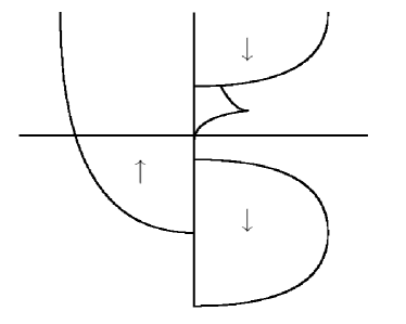
Figure 8: Left: Schematic half-metallic DOS with and without the spin mixing Dowben and Skomski (2004). Right: Schematic half-metallic DOS, and the presence of NQP states, a genuine many-body effect.

Fig. 8 shows also a schematic comparison between this approximation and many-body results. In the tight-binding approach, the distortion of the spin-up and spin-down DOS is presented by the dark regions. The spin mixing gives a non-zero symmetric $N_{\downarrow}(E)$, DOS being weakly modified by thermal fluctuations.

Itoh et al. Itoh et al. (2000) calculated the polarization for a ferromagnet-insulator magnetic tunnel junction with and without spin fluctuations in a thermally randomized atomic potential. The results indicate that the effect of spin fluctuations is significant. The idea of spin fluctuations was further developed by Lezaic et al. Lezaic et al. (2006) by considering the competition between hybridization and thermal spin fluctuation in the prototype HMF NiMnSb.

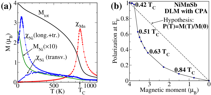
Figure 9: Left: Monte-Carlo results for finite temperature magnetic properties. Right: Polarization at E_F as a function of total spin moment in the DLM picture for NiMn${}_{1-x}^{\uparrow}$Mn${}_{x}^{\downarrow}$Sb calculated with CPA. Lezaic et al. (2006)

.

Figure 9 shows the sublattice susceptibilities computed within a generalized Heisenberg-type Hamiltonian. These results demonstrate that the Ni-sublattice magnetic order is lost already at 50K (this effect is a consequence of weakness of the coupling between the Ni moments and the neighbor atoms), however, neutron diffraction data Hordequin et al. (1997a, b)does not support this scenario. The right hand side of Fig. 9 presents the polarization $P(T)$ calculated in a disordered local moment (DLM) approach Gyorffy et al. (1985), representing the system at finite temperatures in a mean-field way. It is concluded that the thermal collapse of the polarization is connected with a change in hybridization due to the moment fluctuation, the effect of non-collinearity being much milder.

The issue of finite-temperature spin polarization in half-metals remains an open question. Magnons play a crucial role, independently of the theoretical approach. Besides that, a role of phonon modes in the the many-sublattice half-metals is not excluded. Nevertheless, a non-trivial contributions to physics of half-metallic ferromagnets comes from genuine many-body effects. The corresponding first-principle calculations will be presented in Sect.V.

III.4 The tunneling conductance and spin-polarized STM

An useful tool to probe the spin polarization and non-quasiparticle states in HMF is provided by tunneling phenomena Auslender and Irkhin (1985b); Bratkovsky (1998); Auth et al. (2003); Gercsi et al. (2006); Sakuraba et al. (2006b, a); Sakuraba et al. (2007), in particular, by Andreev reflection spectroscopy for a HMF-superconductor tunnel junction Tkachov et al. (2001). The most direct way is probably the measurement of a tunnel current between two pieces of HMF with the opposite magnetization directions.

Let us explain in a simple qualitative way why the NQP states are important for the tunneling transport. To this aim we consider the above-discussed narrow-band saturated Hubbard ferromagnet where the current carriers are the holes in the lowest Hubbard band and the NQP states provide all the spectral weight for the minority spin projection . Suppose we have a tunnel junction with two pieces of this ferromagnet with either parallel (Fig. 29b) or antiparallel (Fig. 29c) magnetization directions. From the one-particle point of view, the spin-conserving tunneling is forbidden in the latter case. However, in the framework of many-particle picture the charge current is a transfer process between an empty site and a single-occupied site rather than the motion of the electron irrespective to the site like in the band theory and therefore the distinction between these two cases (see Fig. 29), is due only to the difference in the densities of states. It means that the estimations of the tunneling magnetoresistance based on simple one-electron picture is too optimistic; even for antiparallel spin orientation of two pieces of the half-metallic ferromagnets in the junction for zero temperature the current is not zero, due to the non-quasiparticle states. More exactly, it vanishes for zero bias since the density of NQP states at the Fermi energy equals to zero. However, it grows with the bias sharply, having the scale of typical magnon energies, i.e., millivolts.

Formally, we can consider a standard tunneling Hamiltonian (see, e.g., Ref. Mahan (1990))

$$\mathcal{H}=\mathcal{H}_{L}+\mathcal{H}_{R}+\sum_{\mathbf{kp}}(T_{\mathbf{kp}}c_{\mathbf{k}\uparrow}^{\dagger}c_{\mathbf{p}\downarrow}+h.c.)$$ (59)

where $\mathcal{H}_{L,R}$ are the Hamiltonians of the left (right) half-spaces, respectively, $\mathbf{k}$ and $\mathbf{p}$ are the corresponding quasimomenta, and spin projections are defined with respect to the magnetization direction of a given half-space (spin is supposed to be conserving in the “global” coordinate system). Carrying out standard calculations of the tunneling current $\mathcal{I}$ in the second order in $T_{\mathbf{kp}}$ one has (cf. Mahan (1990))

$$\mathcal{I}\propto\sum_{\mathbf{kqp}}|T_{\mathbf{kp}}|^{2}[1+N_{\mathbf{q}}-f(t_{\mathbf{p-q}})][f(t_{\mathbf{k}})-f(t_{\mathbf{k}}+eV)]\delta(eV+t_{\mathbf{k}}-t_{\mathbf{p-q}}+\omega_{\mathbf{q}})$$ (60)

where $V$ is the bias voltage.

A very efficient new experimental method is spin-polarized scanning tunneling microscopy (STM) Heinze et al. (2000); Wiesendanger et al. (1990); Kleiber et al. (2000) which enables one to probe directly the spectral density with spin resolution in magnetic systems. The spin-polarized STM should be able to probe the NQP states via their contribution to the differential tunneling conductivity $d\mathcal{I}_{\sigma}/dV\propto N_{\sigma}\left(eV\right)$ Irkhin and Katsnelson (2006). Note that the value $N_{\sigma}(eV)$ vanishes for $|eV|<\hbar\omega_{0}$, where $\hbar\omega_{0}$ is an anisotropy gap in the magnon spectrum Irkhin and Katsnelson (2002), which is small, but could be changed by suitable substitution Attema et al. (2004). Keeping in mind that ferromagnetic semiconductors can be considered as a peculiar case of HFM Irkhin and Katsnelson (1983), an account of NQP states can be important for proper description of spin diodes and transistors Flatte and Vignale (2001); Tkachov et al. (2001).

The above formulas are derived for the usual one-electron density of states at $E_{F}$, which is observed, say, in photoemission measurements. However, the factors which are present in the expression for the tunneling current do not influence the temperature dependence, and therefore these results are valid for spin polarization from tunneling conductance at zero bias in STM Ukraintsev (1996); Irkhin and Katsnelson (2006). Unlike the photoemission spectroscopy which probes only occupied electron states, STM detects the states both above and below $E_{F}$, depending on the sign of bias.

One should keep in mind that sometimes the surface of HMF is not half-metallic; in particular, this is the case of a prototype HMF, NiMnSb de Wijs and de Groot (2001). In such a situation, the tunneling current for minority electrons is due to the surface states only. However, the NQP states can be still visible in the tunneling current via the hybridization of the bulk states with the surface one. This leads to the Fano antiresonance picture which is usually observed in STM investigations of the Kondo effect at metallic surfaces. In such cases the tunneling conductance will be proportional to a mixture of $N_{\sigma}$ and the real part of the on-site Green’s function, $L_{\sigma}$. Surprisingly, in this case the effect of NQP states on the tunneling current can be even more pronounced in comparison with the ideal crystal. The reason is that the analytical continuation of the jump in $N_{\sigma}\left(E\right)$ is logarithm; both singularities are cut at the energy $\overline{\omega};$ nevertheless, the energy dependence of $L_{\sigma}\left(E\right)$ can be pronounced Irkhin and Katsnelson (2006).

STM measurements of electron DOS give also an opportunity to probe bosonic excitations interacting with the conduction electrons. Due to electron-phonon coupling, the derivative $dN_{\sigma}\left(E\right)/dE$ and thus $d^{2}\mathcal{I}_{\sigma}\left(V\right)/dV^{2}$ at $eV=E$ have peaks at the energies $E=\pm\omega_{i}$ corresponding to the peaks in the phonon DOS. According to above treatment (see, e.g., Eq.(42), the same effect should be observable for the case of electron-magnon interaction. However, in the latter case these peaks are essentially asymmetric with respect to the Fermi energy (zero bias) due to asymmetry of the non-quasiparticle contributions. This asymmetry can be used to distinguish phonon and magnon peaks.

Thermoelectric power in the tunnel situation was theoretically investigated in Refs.McCann and Fal’ko (2002, 2003). The relative polarizations of ferromagnetic layers can be manipulated by an external magnetic field, and a large difference occurs for a junction between two ferromagnets with antiparallel and parallel polarizations. This magnetothermopower effect becomes giant in the extreme case of a junction between two half-metallic ferromagnets, since the thermopower is inversely proportional to the area of the maximal cross section of the Fermi surface of minority electrons in the plane parallel to the interface. One has a strong polarization dependence of the thermopower

$$\mathcal{Q}_{AP}=0.64kB/e,\mathcal{Q}_{P}\propto k_{B}^{2}T/(eE_{F})$$ (61)

This result is independent of temperature and of the specific half-metallic material, and it represents a giant magnetothermopower effect, $\Delta\mathcal{Q}\simeq\mathcal{Q}_{AP}=-55\mu$V/K.

III.5 Spin waves

Unlike the Stoner theory, the Hubbard model and other model with electron correlations enable one to describe spin-wave excitations in an itinerant ferromagnet. This was already done in the old approaches based on the random phase approximation (RPA) Herring (1966). To discuss related approaches we present the interaction Hamiltonian in terms of the spin density operators

$$\mathcal{H}_{\mathrm{int}}=\frac{U}{2}\sum_{\mathbf{k}\sigma}c_{\mathbf{k}\sigma}^{\dagger}c_{\mathbf{k}\sigma}-\frac{U}{2}\sum_{\mathbf{q}}(S_{-\mathbf{q}}^{-}S_{\mathbf{q}}^{+}+S_{\mathbf{q}}^{+}S_{-\mathbf{q}}^{-})$$ (62)

where $S_{\mathbf{q}}^{\alpha}$ are the Fourier components of spin density operators. The first term in (62) yields a renormalization of the chemical potential and may be omitted. Writing down the sequence of equations of motion for the spin Green’s function

$$G_{\mathbf{q}}(\omega)=\langle\langle S_{\mathbf{q}}^{+}|S_{-\mathbf{q}}^{-}\rangle\rangle_{\omega}$$ (63)

one derives Irkhin and Katsnelson (1990)

$$G_{\mathbf{q}}(\omega)=\frac{\langle S^{z}\rangle-\Omega_{\mathbf{q}}(\omega)/U}{\omega-\Omega_{\mathbf{q}}(\omega)-\pi_{\mathbf{q}}(\omega)}$$ (64)

where

$$\Omega_{\mathbf{q}}(\omega)=U\sum_{\mathbf{k}}\frac{t_{\mathbf{k+q}}-t_{\mathbf{k}}}{t_{\mathbf{k+q}}-t_{\mathbf{k}}+\Delta-\omega}(n_{\mathbf{k\uparrow}}-n_{\mathbf{k+q\downarrow}})$$ (65)

and the self-energy $\pi$ describes corrections to RPA. Unlike the standard form of RPA,

$$G_{\mathbf{q}}(\omega)=\frac{\Pi_{\mathbf{q}}(\omega)}{1-U\Pi_{\mathbf{q}}(\omega)},$$ (66)

$$\Pi_{\mathbf{q}}(\omega)=\sum_{\mathbf{k}}\frac{n_{\mathbf{k\uparrow}}-n_{\mathbf{k+q\downarrow}}}{\omega+t_{\mathbf{k\uparrow}}-t_{\mathbf{k+q\downarrow}}},$$ (67)

the equivalent representation (64) yields explicitly the magnon (spin-wave) pole

$$\omega_{\mathbf{q}}\simeq\Omega_{\mathbf{q}}(0)=\sum_{\mathbf{k}\sigma}\mathcal{A}_{\mathbf{kq}}^{\sigma}n_{\mathbf{k}\sigma}$$ (68)

where $\mathcal{A}_{\mathbf{kq}}^{\sigma}$ is given by (12). Expanding in $q$ we get $\omega_{\mathbf{q}}=\mathcal{D}_{\alpha\beta}q_{\alpha}q_{\beta}$ where

$$\mathcal{D}_{\alpha\beta}=\frac{U}{\Delta}\sum_{\mathbf{k}}\left[\frac{\partial^{2}t_{\mathbf{k}}}{\partial k_{\alpha}\partial k_{\beta}}(n_{\mathbf{k}\uparrow}+n_{\mathbf{k}\downarrow})-\frac{1}{\Delta}\frac{\partial t_{\mathbf{k}}}{\partial k_{\alpha}}\frac{\partial t_{\mathbf{k}}}{\partial k_{\beta}}(n_{\mathbf{k}\uparrow}-n_{\mathbf{k}\downarrow})\right]$$ (69)

Eq. 69 are spin-wave stiffness tensor components. For a weak ferromagnet ($\Delta\ll E_{F},U$) we have $\mathcal{D}\propto\Delta$. The magnon damping in the RPA is given by

$$\gamma_{\mathbf{q}}^{(1)}(\omega)=-\mathrm{Im~{}}\Omega_{\mathbf{q}}(\omega)=\pi U\Delta\omega\sum_{\mathbf{k}}\left(-\frac{\partial n_{\mathbf{k}\uparrow}}{\partial t_{\mathbf{k}\uparrow}}\right)\delta(\omega-t_{\mathbf{k+q\downarrow}}+t_{\mathbf{k\uparrow}})$$ (70)

$$\gamma_{\mathbf{q}}^{(1)}\equiv\gamma_{\mathbf{q}}^{(1)}(\omega_{\mathbf{q}})\simeq\pi U\Delta\omega_{\mathbf{q}}N_{\uparrow}(E_{F})N_{\downarrow}(E_{F})\theta(\omega_{\mathbf{q}}-\omega_{-})$$ (71)

with $\theta(x)$ being the step function. Here $\omega_{-}=\omega(q^{\ast})$ is the threshold energy which is determined by the condition of entering into the Stoner continuum (decay into the Stoner excitations, i.e. electron-hole pairs), $q^{\ast}$ being the minimal (in $\mathbf{k}$) solution to the equation

$$t_{\mathbf{k+q}^{\ast}\downarrow}=t_{\mathbf{k\uparrow}}=E_{F}$$ (72)

The quantity $\omega_{-}$ determines a characteristic energy scale separating two temperature regions: the contributions of spin waves (poles of the Green’s function 64 dominate at $T<\omega_{-}$, and those of Stoner excitations (its branch cut) at $T>\omega_{-}$.

Although the formal expressions in the $s-d$ exchange model are similar, presence of two electron subsystems leads to some new effects, in particular, to possible occurrence of the “optical mode” pole $\omega\simeq 2|I|S$. The problem of the optical mode formation and its damping was investigated in application to degenerate ferromagnetic semiconductors Auslender and Irkhin (1984a, 1985a); Irkhin and Katsnelson (1985a); Irkhin (1987). Kaplan et al Kaplan et al. (2001) performed exact diagonalization studies of the double exchange model which indicate the existence of continuum states in the single-spin-flip channel that overlap the magnons at very low energies (of order 10^-2 eV) and extend to high energies. This picture differs dramatically from the prevalent view, where there are the magnons, plus the Stoner continuum at the high-energy scale, with nothing in between. Peculiarities of magnons in HMF, especially, in the collossal magnetoresistanse materials, have been recently reviewed in Ref. Zhang et al. (2007).

In the case of weak ferromagnets, the contribution of the branch cut of the spin Green’s function may be approximately treated as that of a paramagnon pole at imaginary $\omega$, and we obtain

$$q^{\ast}=k_{F\uparrow}-k_{F\downarrow}\,,\,\,\,\,\,\,\,\,\,\,\,\,\omega_{-}=\mathcal{D}(k_{F\uparrow}-k_{F\downarrow})^{2}\sim\Delta^{3}\sim T_{C}^{2}/E_{F}$$ (73)

Since $q^{\ast}$ is small, we have at small $q>q^{\ast}$, instead of Eq. (71),

$$\gamma_{\mathbf{q}}^{(1)}(\omega_{\mathbf{q}})\simeq\frac{U\Delta\omega}{q}\frac{\Omega_{0}}{4\pi}(m^{\ast})^{2}\equiv A/q$$ (74)

with $\Omega_{0}$ the lattice cell volume. The estimation (73) holds also for the $\mathit{s-d(f)}$ exchange model with the indirect RKKY-interaction where $\mathcal{D}\sim T_{C}/S\sim I^{2}S/E_{F}$.

The damping at very small $q<q^{\ast}$ (where (70) vanishes) is due to the two-magnon scattering processes. To consider these we have to calculate the function $\pi$ to leading order in the fluctuating part of the Coulomb interaction. Writing down the equation of motion for the Green’s function (63) we obtain

$$\pi_{\mathbf{q}}(\omega) = \sum_{\mathbf{pk}}(A_{\mathbf{kq}}^{\uparrow})^{2}[B(\mathbf{k\uparrow,k+q-p\uparrow,\omega}_{\mathbf{p}}-\omega)+B(\mathbf{k+p\downarrow,k+q\downarrow,\omega}_{\mathbf{p}}-\omega)$$ (75)

$$- B(\mathbf{k+p\downarrow,}\mathbf{k\uparrow,\omega}_{\mathbf{p}})-B(\mathbf{k+q\downarrow,k+q-p\downarrow,p,\omega}_{\mathbf{p}})]$$

where

$$B(\mathbf{k}^{\prime}\mathbf{\sigma}^{\prime},\mathbf{k\sigma},\omega)=\frac{N_{\mathbf{p}}(n_{\mathbf{k}^{\prime}\mathbf{\sigma}^{\prime}}-n_{\mathbf{k\sigma}})+n_{\mathbf{k}^{\prime}\mathbf{\sigma}^{\prime}}(1-n_{\mathbf{k\sigma}})}{\omega-t_{\mathbf{k}^{\prime}\mathbf{\sigma}^{\prime}}+t_{\mathbf{k\sigma}}}$$ (76)

The magnon damping needed is given by the imaginary part of (75),

$$\gamma_{\mathbf{q}}^{(2)}(\omega)=\pi\sum_{\mathbf{kp\sigma}}(A_{\mathbf{kq}}^{\uparrow})^{2}(n_{\mathbf{k\sigma}}-n_{\mathbf{k+q-p\sigma}})\left[N_{\mathbf{p}}-N_{B}(\omega_{\mathbf{p}}-\omega)\right]\delta(\omega+t_{\mathbf{k}}-t_{\mathbf{k+q-p}}-\omega_{\mathbf{p}})$$ (77)

Integration for the isotropic electron spectrum gives Irkhin and Katsnelson (1990)

$$\gamma_{\mathbf{q}}^{(2)}(\omega)=\frac{\Omega_{0}^{2}}{12\pi^{3}}\frac{q^{4}}{4\langle S^{z}\rangle^{2}}\sum_{\sigma}k_{F\sigma}^{2}\times\left\{\begin{array}[]{ll}\omega_{\mathbf{q}}/35&,\qquad T\ll\omega_{\mathbf{q}}\\ (T/4)\left(\ln(T/\omega_{\mathbf{q}})+\frac{5}{3}\right)&,\qquad T\gg\omega_{\mathbf{q}}\end{array}\right.$$ (78)

These results were obtained by Silin and Solontsov within the phenomenological Fermi-liquid theory Silin and Solontsov (1984) and Auslender and Irkhin Auslender and Irkhin (1984a, 1985a) within the $s-d$ exchange model. Golosov Golosov (2000) reproduced the results of Refs.Auslender and Irkhin (1984a, 1985a); Irkhin and Katsnelson (1985a) within the $1/2S$-expansion and performed numerical investigations of the magnon spectrum and damping in the limit of large $|I|$ (double-exchange situation) in application to colossal magnetoresistance compounds.

Real part of (75) describes the temperature dependence of the spin stiffness owing to two-magnon processes (besides the simplest $T^{2}$ -contribution which occurs from the temperature dependence of the Fermi distribution functions in (64). The spin-wave contribution connected with the magnon distribution functions is proportional to $T$. More interesting is the non-analytical many-electron contribution owing to the Fermi functions:

$$\delta\mathcal{D}_{\alpha\beta} = \frac{1}{4\langle S^{z}\rangle^{2}}\sum_{\mathbf{pk}}\frac{\partial t_{\mathbf{k}}}{\partial k_{\alpha}}\frac{\partial t_{\mathbf{k}}}{\partial k_{\beta}}\left[\frac{n_{\mathbf{k}\downarrow}(1-n_{\mathbf{k-p}\uparrow})}{t_{\mathbf{k}}-t_{\mathbf{k-p}}-\omega_{\mathbf{p}}}+\right.$$ (79)

$$\ \ \left.+\frac{n_{\mathbf{k+p}\downarrow}(1-n_{\mathbf{k}\downarrow})}{t_{\mathbf{k+p}}-t_{\mathbf{k}}-\omega_{\mathbf{p}}}-\frac{n_{\mathbf{k+p}\downarrow}(1-n_{\mathbf{k}\uparrow})}{t_{\mathbf{k+p\downarrow}}-t_{\mathbf{k\uparrow}}-\omega_{\mathbf{p}}}-\frac{n_{\mathbf{k}\downarrow}(1-n_{\mathbf{k-p}\downarrow})}{t_{\mathbf{k\downarrow}}-t_{\mathbf{k-p\uparrow}}-\omega_{\mathbf{p}}}\right]$$

Performing integration for parabolic spectra of electrons and magnons yields

$$\delta\mathcal{D}(T)=\left(\frac{\pi\Omega_{0}T}{12\langle S^{z}\rangle m^{\ast}}\right)^{2}\frac{1}{D}\left[\sum_{\sigma}N_{\sigma}^{2}(E_{F})\ln\frac{T}{\omega_{+}}-2N_{\uparrow}(E_{F})N_{\downarrow}(E_{F})\ln\frac{\max(\omega_{-},T)}{\omega_{+}}\right]$$ (80)

with

$$\omega_{\pm}=\mathcal{D}(k_{F\uparrow}\pm k_{F\downarrow})^{2}\,,\,\,\,\,\,\,\,\,\,\,\,\,\,\,\,N_{\sigma}(E_{F})=m^{\ast}\Omega_{0}k_{F}/2\pi^{2}$$ (81)

It should be noted that the correction (80) dominates at low temperatures over the above-mentioned $T^{2}$-correction, which demonstrates an important role of corrections to the RPA approximation. Unfortunately, the $T^{2}\ln T$-term has not yet to be considered at analyzing magnon spectra of ferromagnetic metals. We see that temperature dependences of spin-wave characteristics in conducting magnets differ considerably from those in the Heisenberg model.

III.6 Magnetization and local moments

To treat the problem of magnetic moments in the Hubbard model we consider corrections to the magnetization $\langle S^{z}\rangle$. We have

$$\langle S^{z}\rangle=\frac{n}{2}-\sum_{\mathbf{q}}\langle S_{\mathbf{q}}^{-}S_{\mathbf{q}}^{+}\rangle-\langle\widehat{n}_{i\uparrow}\widehat{n}_{i\downarrow}\rangle$$ (82)

The first average involved in (82) is calculated from the spectral representation of the RPA Green’s function 64:

$$\langle S_{-\mathbf{q}}^{-}S_{\mathbf{q}}^{+}\rangle\,=2S_{0}N_{\mathbf{q}}\,\,\,\,\,\,\,\,\,\,\,\,\,\,\,\,\,\,\,\,\,\,\,\,\,(q<q^{\ast})$$ (83)

$$\langle S_{-\mathbf{q}}^{-}S_{\mathbf{q}}^{+}\rangle\,=\frac{1}{\pi}\int_{-\infty}^{\infty}d\omega\frac{N_{B}(\omega)\gamma_{\mathbf{q}}^{(1)}(\omega)(\Delta-\omega)/U}{[\omega-\mathrm{Re~{}}\Omega_{\mathbf{q}}(\omega)]^{2}+[\gamma_{\mathbf{q}}^{(1)}(\omega)]^{2}}\,\,\,\,\,\,\,\,\,\,\,\,\,(q>q^{\ast})$$ (84)

In contradiction with (82), (83), in the true Bloch spin-wave contribution to magnetization every magnon should decrease $\langle S^{z}\rangle$ by unity. The agreement may be restored by allowing not only the magnon pole, but also branch cut contributions Irkhin and Katsnelson (1990). In the semi-phenomenological manner, it is convenient to introduce “magnon” operators which satisfy on the average the Bose commutation relations:

$$b_{\mathbf{q}}=(2S_{0})^{-1/2}S_{\mathbf{q}}^{+}\,,\,\,b_{\mathbf{q}}^{\dagger}=(2S_{0})^{-1/2}S_{-\mathbf{q}}^{-}\,$$ (85)

Then we have

$$\delta\langle S^{z}\rangle\,=-\sum_{\mathbf{q}}\langle\,\,b_{\mathbf{q}}^{\dagger}b_{\mathbf{q}}\rangle\,=\frac{1}{(2S_{0})}\sum_{\mathbf{q}}\langle S_{-\mathbf{q}}^{-}S_{\mathbf{q}}^{+}\rangle$$ (86)

Performing integration over $\omega$ in (84) at $T$=0 K we obtain

$$\delta\langle S^{z}\rangle\,=-\frac{1}{\pi}\sum_{\mathbf{q}}\frac{\gamma_{\mathbf{q}}^{(1)}}{\omega_{\mathbf{q}}}\ln\frac{W}{\omega_{\mathbf{q}}}$$ (87)

with $W$ being the bandwidth. This contribution of the order of $U^{2}\ln(W/\omega_{+})$ describes zero-point decrease of the magnetization due to the ground-state magnon damping which is owing to the Stoner excitations. For parabolic electron and magnon spectra, neglecting the damping in the denominator of (84) we obtain at low temperatures $T<\omega_{-}$ the dependence $\delta\langle S^{z}\rangle_{cl}\propto U^{2}(T/\omega_{+})^{2}$. For a weak ferromagnet, the temperature correction is proportional to $(T/T_{C})^{2}$, in agreement with the self-consistent renormalization theory Moriya (1985). It should be stressed that the $T^{2}$-correction obtained is much larger than the Stoner contribution of the order of $(T/E_{F})^{2}$. The spin-wave corrections to the local magnetic moment at a site $\langle\mathbf{S}^{2}\rangle=(3/4)(n-2\langle\widehat{n}_{i\uparrow}\widehat{n}_{i\downarrow}\rangle)$ at low $T\ll\omega_{-}$ have a weak dependence $-(T/T_{C})^{5/2}$ Irkhin and Katsnelson (1990). This justifies their neglecting in the above discussion of the magnetization (82).

At high $T>\omega_{-}$ the damping in the denominator dominates at small $q$ in the case of a weak ferromagnet. Taking into account (74) we obtain from (84)

$$\delta\langle S_{-\mathbf{q}}^{-}S_{\mathbf{q}}^{+}\rangle=\frac{\Delta}{\pi U}\int_{-\infty}^{\infty}d\omega N_{B}(\omega)\int_{0}^{\infty}\frac{\omega Aqdq}{(\mathcal{D}q^{2})^{2}+A^{2}\omega^{2}/q^{2}}\propto\left(\frac{T}{E_{F}}\right)^{4/3}$$ (88)

Thus we get from (82) the $T^{4/3}$-contribution to the magnetization, which agrees with the result of the phase transition scaling theory near $T=T_{C}$. For a ferromagnet with well-localized magnetic moments the damping may be neglected and we derive a small correction $\delta\langle S^{z}\rangle_{el}\propto-I^{2}\omega_{-}\ln(T/\omega_{-})~{}$Irkhin and Katsnelson (1996).

Now we discuss a more realistic situation in HMF, in particular in the Heusler alloys. These compounds demonstrate high values of the saturation magnetization and Curie temperature (see Irkhin and Katsnelson (1994); Galanakis and Dederichs (eds.); Ozdogan et al. (2006); Fecher et al. (2006)). The strong ferromagnetism is mainly due to local moments of well-separated Mn atoms. On the other hand, the highest magnetic moment ($6\mu_{B}$) and Curie-temperature (1100K) in the classes of Heusler compounds as well as half-metallic ferromagnets was revealed for Co₂FeSi Wurmehl et al. (2005). It was found empirically that the Curie temperature of Co₂-based Heusler compounds can be estimated from a nearly linear dependence on the magnetic moment Fecher et al. (2006).

High spin polarization and magnetic moment of half-metallic ferromagnets can be treated within the generalized Slater-Pauling rule Galanakis et al. (2002b); Fecher et al. (2006). According to the original formulation by Slater and Pauling, the magnetic moments $m$ of 3d elements and their binary compounds can be described by the mean number of valence electrons $n_{V}$ per atom. A plot of $m$ versus magnetic valence $m(n_{M})$ is called the generalized Slater-Pauling rule, as described by Kübler Kübler (1984). According to Hund’s rule it is often favorable that the majority d states are fully occupied ($n_{d\uparrow}=5$). Starting from $m=2n_{\uparrow}-n_{V}$, this leads to the definition of the magnetic valence as $n_{M}=10-n_{V}$, so that the magnetic moment per atom is given by $m=n_{M}+2n_{sp\uparrow}$.

In the case of localized moments, the Fermi energy is pinned in a deep valley of the minority electron density. This constrains $n_{d\downarrow}$ to be approximately 3, and $m=n_{V}-6-2n_{sp\uparrow}$. HMF are supposed to exhibit a real gap in the minority density of states where the Fermi energy is pinned. Then the number of occupied minority states has to be an integer. Thus, the Slater-Pauling rule will be strictly fulfilled with the spin magnetic moment per atom $m=n_{V}-6$. The situation for the HMF and non-HMF full Heusler alloys is shown in Fig.10.

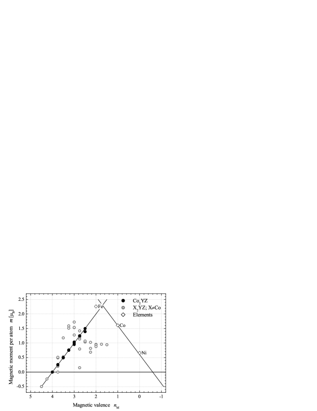
Figure 10: Slater Pauling graph for Heusler compounds Fecher et al. (2006).

For ordered compounds with different kinds of atoms it may be more convenient to consider the total spin magnetic moment $M_{t}$ of all atoms of the unit cell. This quantity scales with the number of valence electron $Z_{t}$: $M_{t}=Z_{t}-18$ for the half-Heusler and $M_{t}=Z_{t}-24$ for the full-Heusler alloys. Thus in both types of compounds the spin magnetic moment per unit cell is strictly integer for the HMF situation. On the other hand, for alloys with non-integer site occupancies like the quaternaries X₂Y_1-xY_xZ the moment may become non-integer depending on the composition, even for the HMF state. The first-principle calculations of the quaternary Heusler alloys Co₂[Cr_1-xMn_x]Al, Co₂Mn[Al_1-xSn_x] and [Fe_1-xCo_x]₂MnAl Galanakis (2004) demonstrated the Slater-Pauling behavior and half-metallic properties. Moreover, this behavior was investigated theoretically in V-based Heusler alloys Mn₂VZ (Z$=$Al, Ga, In, Si, Ge, Sn) which are predicted to demonstrate half-metallic ferrimagnetism Weht and Pickett (1999); Ozdogan et al. (2006); Sasioglu et al. (2005a).

An interesting feature of the half-metallic Heusler alloys is that the Rhodes-Wolfarth ratio $p_{C}/p_{s}$ ($p_{C}$ are the effective moments, $p_{s}$ the saturation moments) can be essentially smaller than unity Irkhin and Katsnelson (1994). Moreover, the effective moment in the paramagnetic state, determined from the paramagnetic susceptibility, decreases appreciably with temperature. We recall that for the Heisenberg magnets (atomic-like magnetic states) we have $p_{C}/p_{s}=1$ and for weak itinerant ferromagnets such as ZrZn₂ $p_{C}/p_{s}\gg 1$, in accordance with the concept of “thermally induced local magnetic moments” Moriya (1985). In the case of conventional strong itinerant ferromagnets (for example, Fe and Ni) this ratio is also greater than unity (for detailed discussion, see Lichtenstein et al. (2001) ). It therefore follows that the inequality $p_{C}/p_{s}<1$ is a striking property of HMF’s, which could be used in their preliminary experimental identification.

This behavior may be explained by that the change of electronic structure. The temperature dependence of magnetic moment in the paramagnetic state may be due to short-range magnetic order (local densities of states are similar to those in the ferromagnetic state). The numerical calculations demonstrate that the reduction in the moments is a consequence of a change in the electron structure as a results of rotation of the magnetic moments as it was demonstrated for Fe and Ni in Ref.Turzhevskii et al. (1990). One would expect such changes to be particularly large in the case of HMF’s and they should be of qualitative nature (smearing out of the hybridization gap because of spin disorder, for a review, see Irkhin and Katsnelson (1994)). From the many-electron model point of view, the decrease of the local moment with increasing temperature is connected with the absence of corrections to ground state magnetization of the type (87). However, such corrections do occur at high temperatures.

III.7 Nuclear magnetic relaxation

Nuclear magnetic resonance (NMR), which is one of most powerful tools for investigating various physical properties, has a number of peculiarities for magnetically ordered materials and especially for HMF. The localized-spin Heisenberg model is inadequate to describe the most interesting systems mentioned above where the role of conduction electrons is essential in magnetic properties. Usually the data on the longitudinal nuclear magnetic relaxation rate $1/T_{1}$ are discussed within itinerant-electron models such as Hubbard model or phenomenological spin-fluctuation theories Ueda and Moriya (1975); Moriya (1985); Ishigaki and Moriya (1996); Moriya (1994); Millis et al. (1990). On the other hand, in the $s-d(f)$ exchange model (well-separated localized and itinerant subsystems) magnetic properties differ essentially from those in the paramagnon regime. We discuss the contributions to $1/T_{1}(T)~{}$owing to electron-magnon interaction for three- and two-dimensional ($3D$ and $2D$) metallic ferromagnets with well-defined local magnetic moments with especial attention to HMF case Irkhin and Katsnelson (2001).

The standard Hamiltonian of the hyperfine interaction, $\mathcal{H}_{hf}=\mathbf{hI,}$ ($h_{\alpha}=A_{\alpha\beta}S_{\beta}$, $\widehat{A}$ is the hyperfine interaction matrix) contains the Fermi (contact) and dipole-dipole contributions, $A_{\alpha\beta}=A^{F}\delta_{\alpha\beta}+A_{\alpha\beta}^{dip}.$ According to Abragam (1961) we have

$$h^{-} = (A^{F}+\frac{1}{3}aF^{(0)})S^{-}+aF^{(2)}S^{+}+2aF^{(1)}S^{z},$$ (89)

$$h^{z} = (A^{F}-\frac{2}{3}aF^{(0)})S^{z}+a(F^{(1)}S^{+}+F^{(1)\ast}S^{-})$$ (90)

where

$$F^{(0)} = \langle(1-3\cos^{2}\theta)/r^{3}\rangle,F^{(1)}=\langle\sin\theta\cos\theta\exp(-i\phi)/r^{3}\rangle,$$

$$F^{(2)} = \langle\sin^{2}\theta\exp(-2i\phi)/r^{3}\rangle,a=-\frac{3}{2}\gamma_{e}\gamma_{n},$$ (91)

$\langle...\rangle$ is the average over the electron subsystem states, $\gamma_{e}$ and $\gamma_{n}$ are gyromagnetic ratios for electron and nuclear moments, respectively. In the case of the local cubic symmetry we have $F^{(a)}=0.$ The Fermi hyperfine interaction is proportional to the electron density at the nucleus and therefore only $s$ states participate in it, the contribution of core $s$ states (which are polarized due to local magnetic moments) being much larger than of conduction electrons. It is just the consequence of considerably smaller localization area (and therefore higher density on nuclei) for the core states. It is obvious that magnetic $f$ or $d$ electrons dominate also in dipole interactions because of large spin polarization. Hence the direct interaction of nuclear spins with that of conduction electrons can be neglected in magnets with well-defined local magnetic moments. Nevertheless, conduction electrons do effect nuclear relaxation via their influence on the local-moment system; besides that, as we shall see below, such contributions possess large exchange enhancement factors.

Using the expressions for $1/T_{1}~{}$and linewidth $1/T_{2}$ in terms of the Green’s functions Moriya (1963)

$$\frac{1}{T_{1}} = -\frac{T}{2\pi}\text{{Im}}\sum_{\mathbf{q}}\langle\langle h_{\mathbf{q}}^{+}|h_{-\mathbf{q}}^{-}\rangle\rangle_{\omega_{n}}/\omega_{n},$$ (92)

$$\frac{1}{T_{2}} = \frac{1}{2T_{1}}-\frac{T}{2\pi}\lim_{\omega\rightarrow 0}\text{{Im}}\sum_{\mathbf{q}}\langle\langle h_{\mathbf{q}}^{z}|h_{-\mathbf{q}}^{z}\rangle\rangle_{\omega}/\omega$$ (93)

($\omega_{n}=\langle h^{z}\rangle\ll T$ is the NMR frequency) we derive

$$\frac{1}{T_{1}} = \frac{T}{2}\{[(A^{F}+\frac{1}{3}aF^{(0)})^{2}+a^{2}|F^{(2)}|^{2}]K^{+-}+4a^{2}|F^{(1)}|^{2}K^{zz}\}$$ (94)

$$\frac{1}{T_{2}} = \frac{1}{2T_{1}}+\frac{T}{2}\{(A^{F}-\frac{2}{3}aF^{(0)})^{2}K^{zz}+a^{2}[2|F^{(1)}|^{2}K^{+-}]\}$$ (95)

$$K^{\alpha\beta}=-(1/\pi)\lim_{\omega\rightarrow 0}\text{{Im}}\sum_{\mathbf{q}}\langle\langle S_{\mathbf{q}}^{+}|S_{-\mathbf{q}}^{-}\rangle\rangle_{\omega}/\omega$$ (96)

Passing to the magnon representation we obtain

$$\langle\langle S_{\mathbf{q}}^{+}|S_{-\mathbf{q}}^{-}\rangle\rangle_{\omega}=2S/[\omega-\omega_{\mathbf{q}}+i\gamma_{\mathbf{q}}(\omega)]$$ (97)

where $\omega_{\mathbf{q}}=2S(J_{\mathbf{q}}-J_{0})+\omega_{0}$ is the magnon frequency, $\gamma_{\mathbf{q}}(\omega)\propto\omega$ is the magnon damping. Then we have

$$K^{+-}=\frac{2S}{\pi\omega_{n}}\sum_{\mathbf{q}}\frac{\gamma_{\mathbf{q}}(\omega_{n})}{\omega_{\mathbf{q}}^{2}}$$ (98)

The damping owing to the one-magnon decay processes can be represented as

$$\gamma_{\mathbf{q}}^{(1)}(\omega)=2\pi I^{2}S\omega\sum_{\mathbf{k}}\delta(t_{\mathbf{k\uparrow}})\delta(t_{\mathbf{k-q\downarrow}}).$$ (99)

where the energy is referred to the Fermi level. The linearity of spin fluctuation damping in $\omega$ is a characteristic property of metals. According to (94) this leads to $T$-linear contributions to $1/T_{1}$ which is the Korringa law. It is important that the simplest expression for the Korringa relaxation

$$1/T_{1}\simeq 1/T_{2}\simeq A^{2}N_{\uparrow}(E_{F})N_{\downarrow}(E_{F})T,$$ (100)

($A$ is an effective hyperfine interaction constant) is practically never applicable for magnetic metals: exchange enhancement factors can change even the order of magnitude of $1/T_{1}$ Moriya (1985); Irkhin and Katsnelson (1994). Accurate expression for the “Korringa” contribution in the case under consideration can be derived by the substitution (98) and (99) into (94).

Apart from three-dimensional case we can consider also two-dimensional HMF keeping in mind, e.g., layered CMR compounds like LaSr₂Mn₂O₇ Nagaev (2001); de Boer and Groot (1999). According to (71), the damping (99) has the threshold value of $q,$ which is determined by the spin splitting $\Delta=2|I|S$, $q^{\ast}=\Delta/v_{F}$ ($v_{F}$ is the electron velocity at the Fermi level), corresponding characteristic temperature and energy scale being $\omega_{-}\sim(\Delta/v_{F})^{2}T_{C}$. After integration for the parabolic electron spectrum the one-magnon damping contribution to (98) takes the form

$$\delta^{(1)}K^{+-}=\frac{N_{\uparrow}(E_{F})N_{\downarrow}(E_{F})}{\mathcal{D}^{2}m^{2}}\times\left\{\begin{tabular}[]{ll}$1/4,$&$D=3$\\ $1/(\pi q^{\ast}),$&$D=2$\end{tabular}\ \ \right.$$ (101)

with $m$ the electron effective mas. Thus in the $3D$ case the factor of $I^{2}$ is canceled, and the factor of $I^{-1}$ occurs in the $2D$ case, so that we obtain a strongly enhanced $T$-linear Korringa-type term (remember that $\mathcal{D}\sim J\sim I^{2}/W$ for the RKKY interaction). This means that the contribution of conduction electrons to $T$-linear relaxation rate via their interaction with localized spins is indeed much more important than the “direct” contribution: perturbation theory in the $s-d$ exchange coupling parameter $I$ turns out to be singular.

In HMF the one-magnon decay processes are absent and electron-magnon (two-magnon) scattering processes should be considered (Sect.III.5). Substituting the corresponding damping into (98) yields for $D=3$

$$\delta^{(2)}K^{+-}=\frac{\Omega_{0}T^{1/2}}{128\pi^{2}Sm^{2}\mathcal{D}^{7/2}}\sum_{\sigma}N_{\sigma}^{2}(E_{F})\times\left\{\begin{tabular}[]{ll}$3\pi^{1/2}\zeta(\frac{3}{2})T,$&$T\ll\omega_{-}$\\ $5.2\omega_{,}$&$T\gg\omega_{-}$\end{tabular}\ {}\right.$$

where $\zeta(z)$ is the Riemann function, $\Omega_{0}$ the lattice cell volume. This contribution can also modify considerably the temperature dependence of $1/T_{1}$ in “usual” ferromagnets, a crossover from $T^{5/2}$ to $T^{3/2}$ dependence of the correction taking place.

For $D=2$ and $T,\omega_{-}\gg\omega_{0},$ small magnon momenta of order of $\left(\omega_{0}/\mathcal{D}\right)^{1/2}$ make the main contribution to (98). On using the high-temperature expression $N_{\mathbf{p}}=T/\omega_{\mathbf{p}}$ one gets

$$\delta^{(2)}K^{+-}=1.23\frac{\Omega_{0}^{3}k_{F}}{8\pi^{4}S\mathcal{D}^{5/2}\omega_{0}^{1/2}}T$$ (102)

Thus in the $2D$ FM case, in contrast with $3D$ one, the relaxation rate $1/T_{1}$ is strongly dependent on the anisotropy gap. It is worthwhile to note an important difference between relaxation processes via phonons and via magnons. The main difference is due to the gap in magnon spectrum. Usually $\omega_{0}>\omega_{n}$ and therefore one-magnon processes contribute to the relaxation rate due to magnon damping only (cf. discussion of the phonon-induced relaxation processes in Ref.Abragam (1961)). However, the mechanisms of magnon damping in magnetic dielectrics (magnon-magnon interactions) are different from those in magnetic metals and degenerate semiconductors Auslender and Irkhin (1984a, 1985a).

III.8 Thermodynamic properties

Consider the renormalization of electronic specific heat in an itinerant ferromagnet due to interaction with spin fluctuations. Integration in (8), (9) at $T=0~{}$ gives

$$\mathrm{Re}\Sigma_{\sigma}(k_{F\sigma},E)=-\frac{U\Delta}{\omega_{+}-\omega_{-}}N_{-\sigma}(E_{F})\sum_{\alpha=\pm}\alpha(E-\omega_{\alpha})\ln\frac{|E-\omega_{\alpha}|}{W}$$

Then the inverse residue of the electron Green’s function, $1/Z_{\mathbf{{k}\sigma}}(E)=1-(\partial/\partial E)\mathrm{Re}\Sigma_{\mathbf{k}\sigma}(E)$, which determines the renormalization of the electron effective mass owing to the electron-magnon interaction, contains a logarithmic factor. We obtain for the coefficient at the linear term in the electronic specific heat at $T\ll\omega_{-}$

$$\gamma_{\sigma}=\gamma_{\sigma}^{(0)}/Z_{\sigma}(k_{F\sigma},E_{F})=\frac{\pi^{2}}{3}N_{\sigma}(E_{F})\left[1+\frac{U\Delta}{\omega_{+}-\omega_{-}}N_{-\sigma}(E_{F})\ln\frac{\omega_{+}}{\omega_{-}}\right]$$ (103)

For weak itinerant ferromagnets we have

$$\ln\frac{\omega_{+}}{\omega_{-}}\simeq-2\ln(UN(E_{F})-1)$$ (104)

so that the we have a paramagnon enhancement of the specific heat, the numerical factor in (103) being inexact in this limit because of neglecting longitudinal spin fluctuations (see Moriya (1985)). On the other hand, we have a considerable enhancement of specific heat owing to spin fluctuations strong ferromagnets which is really observed in a number of systems.

Other thermodynamic properties may be treated by calculating the free energy of the system. The spin-wave contribution to the free energy has the form, usual for the Bose excitations with the square dispersion law and is proportional to $(T/T_{C})^{5/2}$. At low $T<\omega_{-}$ the many-electron (branch cut) contribution reads

$$F_{\mathrm{el}}=\frac{1}{2S_{0}}\sum_{\mathbf{q>q}^{\ast}}\omega_{\mathbf{q}}\langle S_{-\mathbf{q}}^{-}S_{\mathbf{q}}^{+}\rangle\,\simeq U\Delta\sum_{\mathbf{kk}^{\prime}}\frac{n_{\mathbf{k}^{\prime}\downarrow}(1-n_{\mathbf{k\uparrow}})}{t_{\mathbf{k\uparrow}}-t_{\mathbf{k}^{\prime}\downarrow}+\omega_{\mathbf{k-k}^{\prime}}}$$ (105)

Differentiating (105) over $T$ one obtains

$$\delta C_{\mathrm{el}} = -\frac{\partial}{\partial T}\delta F_{el}(T)$$ (106)

$$= U^{2}\frac{2\langle S^{z}\rangle}{\omega_{+}-\omega_{-}}N_{\uparrow}(E_{F})N_{\downarrow}(E_{F})\frac{2\pi^{2}}{3}T\ln\frac{\omega_{+}}{\max(\omega_{-},T)}$$

Thus at $T\gg\omega_{-}$ we have instead of (103) the $T\ln T$-dependence of specific heat.

As one can see from (103), the enhancement of effective mass and electronic specific heat owing to spin fluctuations is absent in the half-metallic state. We shall demonstrate that the specific heat of a conducting ferromagnet may contain spin-fluctuation contributions of another nature. Write down a general expression for the specific heat in the $s-d$ exchange model in terms of the total energy

$$C(T) = \frac{\partial\langle\mathcal{H}\rangle}{\partial T}=\frac{\partial}{\partial T}\int dEEf(E)N_{t}(E)$$ (107)

$$= \frac{\pi^{2}}{3}N_{t}(E)T+\int dEEf(E)\frac{\partial}{\partial T}N_{t}(E,T)$$

where

$$N_{t}(E)=-\frac{1}{\pi}\sum_{\mathbf{k}\sigma}\text{{Im}}G_{\mathbf{k}\sigma}(E)$$

The first term in the right-hand side of (107) yields the standard result of the Fermi-liquid theory. The second term is due to the energy dependence of the density of states. Such a dependence occurs in the conducting ferromagnet owing to non-quasiparticle (incoherent) states. Using again the expressions for the self-energies (8), (9) we derive Irkhin and Katsnelson (1990)

$$\delta C_{\sigma}(T)=2\sigma I^{2}\langle S^{z}\rangle\sum_{\mathbf{kq}}\frac{f(t_{\mathbf{k+q},-\sigma}-\sigma\omega_{\mathbf{q}})}{(t_{\mathbf{k+q},-\sigma}-t_{\mathbf{k},\sigma})^{2}}\frac{\partial}{\partial T}n_{\mathbf{k+q},-\sigma}$$ (108)

Since at low temperatures $f(t_{\mathbf{k+q},\downarrow}-\omega_{\mathbf{q}})=1,f(t_{\mathbf{k+q},\uparrow}-\omega_{\mathbf{q}})=0$, the non-quasiparticle states with $\sigma=\downarrow$ do not contribute to linear specific heat since they are empty at $T$=0 K. In the half-metallic state the non-quasiparticle contributions (107) with $\sigma=\uparrow$ are present for $I<0$ only, and we obtain

$$\delta C_{\uparrow}(T)=\frac{2\pi^{2}}{3}I^{2}\langle S^{z}\rangle N_{\downarrow}(E_{F})T\sum_{\mathbf{k}}\frac{1}{(t_{\mathbf{k\uparrow}}-E_{F})^{2}}$$ (109)

To avoid misunderstanding, it should be stressed that presence of such contributions to specific heat means inapplicability of the Fermi-liquid description in terms of dynamical quasiparticles only, which are determined by poles of Green’s functions. It may be shown rigorously that the entropy of interacting Fermi systems at low $T$ is expressed in terms of Landau quasiparticles with the energies, determined as variational derivatives of the total energy with respect to occupation numbers Carneiro and Pethick (1975). Thus, even in the presence of non-pole contributions to the Green’s functions, the description of thermodynamics in terms of statistical quasiparticles Carneiro and Pethick (1975) holds. (However, the quasiparticle description is insufficient for spectral characteristics, e.g., optical and emission data.) The anomalous $\gamma T$-term is determined by the difference of the spectra of statistical and dynamical quasiparticles.

Similar contributions to specific heat in the Hubbard model with strong correlations are discussed in the paper Irkhin and Katsnelson (1990) too. They dominate in the enhancement of specific heat for half-metallic ferromagnets and may be important, besides the effective mass enhancement (103), for “usual” magnets with well-defined local moments.

III.9 Transport properties

Transport properties of HMF are the subject of numerous experimental investigations (see, e.g., recent works for CrO₂ Rabe et al. (2002) and NiMnSb Borca et al. (2001), and the reviews Irkhin and Katsnelson (1994); Ziese (2002); Nagaev (2001)). At the same time, the theoretical interpretation of these results is still a problem. As for electronic scattering mechanisms, the most important difference between HMF and “standard” itinerant electron ferromagnets like iron or nickel is the absence of one-magnon scattering processes in the former case Irkhin and Katsnelson (1994).

Since the states with one spin projection only exist at the Fermi level and one-magnon scattering processes are forbidden in the whole spin-wave region, the corresponding $T^{2}$-term in resistivity is absent in the case of a half-metallic ferromagnets. This seems to be confirmed by comparing experimental data on resistivity of Heusler alloys TMnSb (T = Ni, Co, Pt, Cu, Au) and PtMnSn Otto et al. (1989) (see also discussion in Sect. V.1.1). The $T^{2}$-contribution from one-magnon processes to resistivity for half-metallic systems (T = Ni, Co, Pt) was really not picked out, whereas the dependences $\rho(T)$ for “usual” ferromagnets were considerably steeper.

Two-magnon scattering processes have been considered many years ago, the temperature dependence of resistivity obtained being $T^{7/2}$ Roesler (1965); Hartman-Boutron (1965). The obtained temperature dependence of the resistivity has the form $T^{7/2}$. At low enough temperatures the first result fails and should be replaced by $T^{9/2}$ Lutovinov and Reizer (1979); the reason is the compensation of the transverse and longitudinal contributions in the long-wavelength limit which is a consequence of the rotational symmetry of the $s-d$ exchange Hamiltonian Grigin and Nagaev (1974); Nagaev (1983); Auslender et al. (1983). We discuss effects of interaction of current carriers with local moments are investigated in the standard $s-d$ exchange model in the spin-wave region.

$$\mathcal{H} = \mathcal{H}_{0}-I(2S)^{1/2}\sum_{\mathbf{kq}}(c_{\mathbf{k}\uparrow}^{\dagger}c_{\mathbf{k}+\mathbf{q}\downarrow}b_{\mathbf{q}}^{\dagger}+h.c.)$$ (110)

$$\ \ \ \ \ +I\sum_{\mathbf{kqp}\sigma}\sigma c_{\mathbf{k}\sigma}^{\dagger}c_{\mathbf{k+q-p}\sigma}b_{\mathbf{q}}^{\dagger}b_{\mathbf{p}}$$

The zero-order Hamiltonian includes non-interacting electrons and magnons,

$$\mathcal{H}_{0} = \sum_{\mathbf{k}\sigma}E_{\mathbf{k}\sigma}c_{\mathbf{k}\sigma}^{\dagger}c_{\mathbf{k}\sigma}+\sum_{\mathbf{q}}\omega_{\mathbf{q}}b_{\mathbf{q}}^{\dagger}b_{\mathbf{q}},$$ (111)

$$E_{\mathbf{k}\sigma} = t_{\mathbf{k}}-\sigma\Delta/2,\omega_{\mathbf{q}}=2S(J_{0}-J_{\mathbf{q}}),$$

with $\Delta=2IS$ being the spin splitting which is included in $\mathcal{H}_{0}$. In the half-metallic case the spin-flip processes do not work in the second order in $I$ since the states with one spin projection only are present at the Fermi level. At the same time, we have to consider the renormalization of the longitudinal processes in higher orders in $I$ (formally, we have to include the terms up to the second order in the quasiclassical small parameter $1/S$). To this end we can eliminate from the Hamiltonian the terms which are linear in the magnon operators by using the canonical transformation Grigin and Nagaev (1974); Nagaev (1983). Then we obtain the effective Hamiltonian

$$\widetilde{\mathcal{H}}=\mathcal{H}_{0}+\frac{1}{2}\sum_{\mathbf{kqp}\sigma}(\mathcal{A}_{\mathbf{kq}}^{\sigma}+\mathcal{A}_{\mathbf{k+q-p,q}}^{\sigma})c_{\mathbf{k}\sigma}^{\dagger}c_{\mathbf{k+q-p}\sigma}b_{\mathbf{q}}^{\dagger}b_{\mathbf{p}}$$ (112)

Here $\mathcal{A}_{\mathbf{kq}}^{\sigma}$ is the $s-d$ scattering amplitude which is defined by (12) ($U\rightarrow I$). More general interpolation expression for the effective amplitude, which does not assume the smallness of $|I|$ or $1/2S$ was obtained in Ref.Auslender et al. (1983) by a variational approach.

The most general and rigorous method for calculating the transport relaxation time is the use of the Kubo formula for the conductivity $\sigma_{xx}$ Kubo (1957) (see details in Ref.Irkhin and Katsnelson (2002)):

$$\sigma_{xx}=\beta\int_{0}^{\beta}d\lambda\int_{0}^{\infty}dt\exp(-\varepsilon t)\langle j_{x}(t+i\lambda)j_{x}\rangle$$ (113)

where $\beta=1/T,$ $\varepsilon\rightarrow 0,$

$$\mathbf{j}=-e\sum_{\mathbf{k}\sigma}\mathbf{v}_{\mathbf{k}\sigma}c_{\mathbf{k}\sigma}^{\dagger}c_{\mathbf{k}\sigma}$$ (114)

is the current operator, $\mathbf{v}_{\mathbf{k}\sigma}=\partial E_{\mathbf{k}\sigma}/\partial\mathbf{k}$ is the electron velocity. Representing the total Hamiltonian in the form $\mathcal{H}=\mathcal{H}_{0}+\mathcal{H}^{\prime}$, the correlator in (113) may be expanded in the perturbation $\mathcal{H}^{\prime}$ Nakano (1957); Mori (1965). In the second order we obtain for the electrical resistivity

$$\rho_{xx}=\sigma_{xx}^{-1}=\frac{T}{\langle j_{x}^{2}\rangle^{2}}\int_{0}^{\infty}dt\langle[j_{x},\mathcal{H}^{{}^{\prime}}(t)][\mathcal{H}^{{}^{\prime}},j_{x}]\rangle$$ (115)

where $\mathcal{H}^{\prime}(t)$ is calculated with the Hamiltonian $\mathcal{H}_{0}$.

In the HFM situation the band states with one spin projection only, $\sigma=\mathrm{sign}I,$ are present at the Fermi level Irkhin and Katsnelson (1994). We consider the case $I>0,$ $\sigma=+$ and omit the spin indices in the electron spectrum to obtain for the transport relaxation time $\tau$ defined by $\sigma_{xx}=e^{2}\langle(v^{x})^{2}\rangle\tau$

$$\frac{1}{\tau} = \frac{\pi}{4T}\sum_{\mathbf{kk}^{\prime}\mathbf{q}}(v_{\mathbf{k}}^{x}-v_{\mathbf{k}^{\prime}}^{x})^{2}(\mathcal{A}_{\mathbf{kq}}^{\uparrow}+\mathcal{A}_{\mathbf{k}^{\prime}\mathbf{,q-k}^{\prime}\mathbf{+k}}^{\uparrow})^{2}N_{\mathbf{q}}(1+N_{\mathbf{q-k}^{\prime}+\mathbf{k}})$$ (116)

$$\ \ \ \ \ \ \ \ \ \times n_{\mathbf{k}}(1-n_{\mathbf{k}^{\prime}})$$

$$\times\delta(t_{\mathbf{k}^{\prime}}-t_{\mathbf{k}}-\omega_{\mathbf{q}}+\omega_{\mathbf{q-k}^{\prime}+\mathbf{k}})\left/\sum_{\mathbf{k}}(v_{\mathbf{k}}^{x})^{2}\delta(t_{\mathbf{k}})\right.$$

Averaging over the angles of the vector $\mathbf{k}$ leads to the result $1/\tau\propto I^{2}\Phi$ with

$$\Phi=\sum_{\mathbf{pq}}f_{\mathbf{pq}}\frac{\beta(\omega_{\mathbf{p}}-\omega_{\mathbf{q}})|\mathbf{p-q}|}{\exp\beta\omega_{\mathbf{p}}-\exp\beta\omega_{\mathbf{q}}}(1+N_{\mathbf{q}})(1+N_{\mathbf{p}})$$ (117)

where $f_{\mathbf{pq}}=1$ for $p,q\gg q^{\ast}$ and

$$f_{\mathbf{pq}}=\frac{[\mathbf{p\times q]}^{2}}{(\mathbf{p-q)}^{2}(q^{\ast})^{2}}\,\,\,(p,q\ll q^{\ast}).$$ (118)

As discussed before, the wavevector $q^{\ast}$ determines the boundary of the region where $\mathbf{q}$-dependence of the amplitude become important, so that $t(\mathbf{k+q})-t(\mathbf{k})\simeq\Delta$ at $q\simeq q^{\ast}$. In the case $q<q^{\ast}$ the simple perturbation theory fails and we have to take into account the spin splitting by careful collecting the terms of higher orders in $I$. In the simple one-band model of HMF where $E_{F}<\Delta$ one has $q^{\ast}\sim\sqrt{\Delta/W}$ ($W$ is the conduction bandwidth) Grigin and Nagaev (1974); Nagaev (1983). The quantity $q^{\ast}$ determines a characteristic temperature and energy scale $T^{\ast}=\mathcal{D}(q^{\ast})^{2}\propto\mathcal{D}({\Delta/}W).~{}$

When estimating temperature dependences of resistivity one has to bear in mind that each power of $p$ or $q$ gives $T^{1/2}.$ At very low temperatures $T<T^{\ast}$ small quasimomenta $p,q<q^{\ast}$ yield main contribution to the integrals and

$$\rho(T)\propto(T/T_{C})^{9/2}$$ (119)

Such a dependence was obtained in the narrow-band case (double-exchange model with large $|I|$), where the scale $T^{\ast}$ is absent Kubo and Ohata (1972), and by the diagram approach in the broad-band case Lutovinov and Reizer (1979). At the same time, at $T>T^{\ast}$ the function $f_{\mathbf{pq}}$ in Eq. (117) can be replaced by unity to obtain

$$\rho(T)\propto(T/T_{C})^{7/2}$$ (120)

Generally speaking, $q^{\ast}$ may be sufficiently small provided that the energy gap is much smaller than $W$, which is the case for real HMF systems. We consider the model of HMF spectrum (49) where the majority-spin band is metallic and the minority-spin is semiconducting. For the temperatures $T\ll T_{C}$ both characteristic $q$ and $p$ are small in comparison with the inverse lattice constant and we can put

$$\mathcal{A}_{\mathbf{kq}}^{\sigma}=\frac{1}{2S}\left(t_{\mathbf{k}\downarrow}-t_{\mathbf{k}\uparrow}\right)\frac{t_{\mathbf{k+q}\uparrow}-t_{\mathbf{k}\uparrow}}{t_{\mathbf{k+q}\uparrow}-t_{\mathbf{k}\downarrow}}$$ (121)

The wavevector $q^{\ast}$ determines the boundary of the region where $\mathbf{q}$-dependence of the amplitude become important, so that $q^{\ast}=\Delta/v_{F}$ (the same value as for the spin polarization problem). The corresponding characteristic temperature and energy scale is

$$T^{\ast}=\mathcal{D}(q^{\ast})^{2}\propto\mathcal{D}({\Delta/}W)^{2}$$ (122)

which coincides with the case of an usual ferromagnetic metal. The above temperature dependences of resistivity are not changed Irkhin and Katsnelson (2002).

Now we treat the two-dimensional ($2D$) situation which may be appropriate for layered manganites Nagaev (2001); de Boer and Groot (1999). At low temperatures we obtain

$$\rho(T<T^{\ast})\propto(T/T_{C})^{7/2}$$ (123)

At the same time, for $T>T^{\ast}$ we obtain after replacing the scattering amplitude by unity a logarithmically divergent integral which should be cut at $T^{\ast}$. Thus we get

$$\rho(T>T^{\ast})\propto(T/T_{C})^{5/2}\ln(T/T^{\ast})$$ (124)

To discuss the magnetoresistivity we have to introduce the gap in the magnon spectrum, $\omega_{\mathbf{q\rightarrow}0}=\mathcal{D}q^{2}+\omega_{0}.$ Provided that the external magnetic field $H$ is large in comparison with the anisotropy gap, $\omega_{0}$ is proportional to $H$. In the $3D$ case the resistivity at $T<T^{\ast}$ is linear in magnetic field,

$$\rho(T,H)-\rho(T,0)\propto-\omega_{0}T^{7/2}/T_{C}^{9/2}$$ (125)

The situation at $T>T^{\ast}$ is more interesting since the quantity $\partial\Phi/\partial\omega_{0}$ contains a divergence which is cut at $\omega_{0}$ or $T^{\ast}$. We have at $T>\omega_{0},T^{\ast}$

$$\delta\rho(T,H)\propto-\frac{T^{3}\omega_{0}}{[\max(\omega_{0},T^{*})]^{1/2}}$$ (126)

(of course, at $T<\omega_{0}$ the resistivity is exponentially small). A negative $H$-linear magnetoresistance was observed recently in CrO₂ Rabe et al. (2002).

The discovery of giant magnetoresistance (GMR) lead to tremendous activity to understand and develop technology based on high-density magnetic recording Zutic et al. (2004). Giant magnetoresistance for metallic multilayers (superlattices) containing HMF was first predicted in Irkhin and Katsnelson (1994). NiMnSb-based spin-valve structures using Mo spacer layers NiMnSb/Mo/NiMnSb/SmCo₂ were successfully produced Hordequin et al. (1998). The associated GMR exhibits a clear spin-valve contribution about $\Delta R/R\approx 1\%$ Hordequin et al. (1998). One of the limiting factor for such a small value is the large resistivity of the Mo layer which determines limited flow of active electrons exchanged between the two ferromagnetic layers without being scattered. The giant tunneling magnetoresistance differs by use of dielectric spacer instead of metallic one. The GMR in tunnel junctions based on HMF was considered theoretically in Ref. de Groot et al. (1983a); Tkachov et al. (2001) and recently this issue became a subject of intensive experimental investigations Sakuraba et al. (2006b, a); Sakuraba et al. (2007); Gercsi et al. (2006); Rybchenko et al. (2006).

It is important that NQP states do not contribute to the temperature dependence of the resistivity for pure HMF. An opposite conclusion was made by Furukawa Furukawa (2000). He attempted to calculate low-temperature resistivity of half-metals with account of the non-rigid-band behavior of the minority band due to spin fluctuations at finite temperatures and derived that the unconventional one-magnon scattering process give $T^{3}$-dependence in resistivity. However, this calculation was not based on a consistent use of the Kubo formula and, in our opinion, can be hardly justified.

On the contrary, impurity contributions to transport properties in the presence of potential scattering are determined mainly by the NQP states Irkhin et al. (1994, 1989); Irkhin and Katsnelson (1994)). To second order in the impurity potential $\mathcal{U}$ we derive after neglecting vertex corrections and averaging over impurities we obtain for the transport relaxation time

$$\delta\tau_{\mathrm{imp}}^{-1}(E)=-2\mathcal{U}^{2}\mathrm{Im}\sum_{\mathbf{p}}G_{\mathbf{p}\sigma}^{(0)}(E)$$ (127)

where is the exact Green’s function for the ideal crystal. Thus the contributions under consideration are determined by the energy dependence of the density of states $N(E)$ for the interacting system near the Fermi level. The most nontrivial dependence comes from the non-quasiparticle (incoherent) states with the spin projection $-\sigma=-\mathrm{sign}I,$ which are present near $E_{F}$. Near the Fermi level the NQP contribution is determined by the magnon density of states $g(\omega)$ and follows a power law,

$$\delta N_{\mathrm{incoh}}(E)\propto\int_{0}^{\sigma E}d\omega g(\omega)\propto|E|^{\alpha}\theta(\sigma E)\,\,(|E|\ll\overline{\omega}).$$ (128)

Here $\theta(x)$ is the step function, $E$ is referred to $E_{F}$; we have $\alpha=3/2$ and $\alpha=1$ for $3D$ and $2D$ cases, respectively. The corresponding correction to resistivity reads

$$\frac{\delta\rho_{\mathrm{imp}}(T)}{\rho^{2}} = -\delta\sigma_{\mathrm{imp}}(T)$$ (129)

$$\propto -\mathcal{U}^{2}\int dE\left(-\frac{\partial f(E)}{\partial E}\right)\delta N_{\mathrm{incoh}}(E)\propto T^{\alpha}$$

The contribution of the order of $T^{\alpha}$ with $\alpha\simeq 1.65$ (which is not too far from 3/2) was observed in the temperature dependence of the resistivity for NiMnSb Borca et al. (2001) above 100K. The half-metallic properties above 100K are being challanged, however. The incoherent contribution to magnetoresistivity is given by

$$\delta\rho_{\mathrm{imp}}(T,H)\propto\omega_{0}\partial\delta N_{\mathrm{incoh}}(\sigma T)/\partial T\propto\omega_{0}T^{\alpha-1},$$ (130)

so that we obtain a temperature-independent term in the $2D$ case.

The correction to thermoelectric power, which is similar to (129), reads (cf. Ref.Irkhin et al. (1994, 1989)):

$$\delta\mathcal{Q}(T)\propto\frac{1}{T}\int dE(-\partial f(E)/\partial E)E\delta N(E)$$ (131)

Besides that, an account of higher orders in impurity scattering leads to the replacement of the impurity potential $V$ by the $T$-matrix. For the point-like scattering the latter quantity is given by

$$T(E)=\frac{\mathcal{U}}{1-\mathcal{U}\mathcal{R}(E)},\mathcal{R}(E)=\sum_{\mathbf{k}}G_{\mathbf{k}\sigma}(E).$$ (132)

Expanding (132) yields also the term

$$\delta\mathcal{Q}(T)\propto\frac{1}{T}\int dE(-\partial f(E)/\partial E)E\mathrm{Re}\delta\mathcal{R}(E)$$ (133)

with $\delta\mathcal{R}(E)$ being obtained by analytical continuation from $\delta N(E).$ Thus we have $\delta\mathcal{Q}(T)\propto T^{3/2}$.

III.10 X-ray absorption and emission spectra. Resonant x-ray scattering

The NQP contributions in the presence of the potential $U,$ that is induced by the impurity at a lattice site, can be treated in the $s-d$ exchange model in the representation (23). The impurity potential results in the NQP contribution to this quantity being enhanced for $\mathcal{U}<0$ and suppressed for $\mathcal{U}>0$. These results can be used to consider the manifestations of NQP states in the core level spectroscopy Irkhin and Katsnelson (2005a).

Various spectroscopy techniques such as x-ray absorption, x-ray emission, and photoelectron spectroscopies (xas, xes, and xps, correspondingly) give an important information about the electronic structure of HMF and related compounds, i.e. ferromagnetic semiconductors and colossal magnetoresistance materials (see, e.g., Refs. Yarmoshenko et al. (1998); Yablonskikh et al. (2001); Kurmaev et al. (2003); Wessely et al. (2003)). It is well known Mahan (1990) that many-body effects (e.g., dynamical core hole screening) can be important for the core level spectroscopy even when the system is not strongly correlated in the initial state. Therefore it is very interesting to study the interplay of these effects and NQP states which are of essentially many-body origin themselves.

To consider the core level problem in HMF we use the Hamiltonian of the $s-d$ exchange model in the presence of the external potential $\mathcal{U}$ induced by the core hole,

$$\mathcal{H}^{\prime}=\varepsilon_{0}f^{\dagger}f+\mathcal{U}\sum_{\mathbf{kk}^{\prime}\sigma}c_{\mathbf{k}\sigma}^{\dagger}c_{\mathbf{k}^{\prime}\sigma}f^{\dagger}f$$ (134)

where $f^{\dagger},f$ are core hole operators, $\mathcal{U}<0$. X-ray absorption and emission spectra are determined by the Green’s function Mahan (1990)

$$G_{\mathbf{kk}^{\prime}}^{\sigma}(E)=\langle\langle c_{\mathbf{k}\sigma}f|f^{\dagger}c_{\mathbf{k}^{\prime}\sigma}^{\dagger}\rangle\rangle_{E}$$ (135)

As follows the investigation of the sequence of equations of motion Irkhin and Katsnelson (2005a), in the ladder approximation the spectral density for two-particle Green’s function $G_{\mathbf{kk}^{\prime}}^{\sigma}(E)~{}$is equivalent to the one-particle spectral density in the presence of the core hole potential $\mathcal{U}$ (note that the ladder approximation is inadequate to describe the xas edge singularity in a close vicinity of the Fermi level Mahan (1990)). Thus the core hole problem is intimately connected with the impurity problem.

Since xas probes empty states and xes occupied states, the local DOS

$$N_{\mathrm{loc}}^{\sigma}(E)=-\frac{1}{\pi}\mathrm{Im}G_{00}^{\sigma}(E)$$ (136)

describes the absorption spectrum for $E>E_{F}$ and emission spectrum for $E<E_{F}.$ To take into account the core level broadening a finite damping $\delta$ should be introduced Irkhin and Katsnelson (2005a). For small band filling the “exciton effects” (strong interaction with the core hole) result in a considerable enhancement of NQP contributions to the spectra in comparison with those to DOS. The results for semielliptic bare band are shown in Figs.11,12.

Figure 11: The local density of states $N_{\mathrm{loc}}^{\downarrow}(E)$ (solid line) for a half-metallic ferromagnet with $S=1/2,I=0.3,\delta=0.01$ in the presence of the core hole potential $\mathcal{U}=-0.2.$ The dashed line shows the DOS $N_{\downarrow}(E)$ for the ideal crystal. The value of $E_{F}$ calculated from the band bottom is 0.15.

Figure 12: The local density of states $N_{\mathrm{loc}}^{\uparrow}(E)$ (solid line) for a half-metallic ferromagnet with $S=1/2,I=-0.3,\delta=0.01$ in the presence of the core hole potential $\mathcal{U}=-0.3.$ The dashed line shows the DOS $N_{\uparrow}(E)$ for the ideal crystal. The value of $E_{F}$ calculated from the band bottom is 0.15.

To probe the “spin-polaron” nature of the NQP states more explicitly, it would be desirable to use spin-resolved spectroscopical methods such as x-ray magnetic circular dichroism (XMCD, for a review see Ref. Ebert (1996)). Owing to interference of electron-magnon scattering and “exciton” effects (interaction of electrons with the core hole), the NQP contributions to x-ray spectra can be considerably enhanced in comparison with those to DOS of the ideal crystal. Thus the core level (x-ray absorption, emission and photoelectron) spectroscopy might be an efficient tool to investigate the NQP states in electron energy spectrum.

Now we consider NQP effects in resonant x-ray scattering processes. It was observed recently Kurmaev et al. (2003) that the elastic peak of the x-ray scattering in CrO₂ is observed which is more pronounced than in usual Cr compounds, e.g., in elemental chromium. The authors of this work have put forward some qualitative arguments that the NQP states may give larger contributions to resonant x-ray scattering than usual itinerant electron states. Here we can treat this question quantitatively and estimate explicitly the corresponding enhancement. The intensity of resonant x-ray emission induced by the photon with the energy $\omega$ and polarization $q$ is given by the Kramers-Heisenberg formula

$$I_{q^{\prime}q}(\omega^{\prime},\omega)\propto\sum_{n}\left|\sum_{l}\frac{\langle n|C_{q^{\prime}}|l\rangle\langle l|C_{q}|0\rangle}{E_{0}+\omega^{\prime}-E_{l}-i\Gamma_{l}}\right|^{2}\delta(E_{n}+\omega^{\prime}-E_{0}-\omega)$$ (137)

Here $q^{\prime}$ and $\omega^{\prime}$ are the polarization and energy of the emitted photon, $|n\rangle,|0\rangle$ and $|l\rangle$ are the final, initial and intermediate states of the scattering system, respectively, $E_{i}$ are the corresponding energies, $C_{q}$ is the operator of the dipole moment for the transition, which is proportional to $fc+c^{\dagger}f^{\dagger}$. Assuming for simplicity that $\Gamma_{l}$ does not depend on the intermediate state, $\Gamma_{l}=\Gamma$, and taking into account only the main x-ray scattering channel (where the hole is filled from the conduction band) one obtains Sokolov et al. (1977)

$$I_{\omega^{\prime}}\propto\left|\sum_{\sigma}G_{00}^{\sigma}(z)\right|^{2}$$ (138)

where $z=\omega^{\prime}-E_{0}+i\Gamma.$ Owing to a jump in the DOS at the Fermi level, the NQP part of the Green’s function contains a large logarithm $\ln(W/z)$ at small $z$. It means that the corresponding contribution to the elastic x-ray scattering intensity ($\omega^{\prime}=E_{0}$) is enhanced by a factor of $\ln^{2}(W/\Gamma),$ which makes a quantitative estimation for the qualitative effect discussed in Ref. Kurmaev et al. (2003). Of course, the smearing of the jump in the density of NQP states by spin dynamics is irrelevant provided that $\Gamma\gg\overline{\omega}$ ($\overline{\omega}$ is a characteristic magnon frequency).

IV Modern first-principle calculations

IV.1 Different functional schemes

In this section we review contemporary approaches to the electronic structure calculations with taking into account correlation effects. Model considerations discussed above demonstrate relevance of the correlation effects (such as electron-magnon interactions) for physics of half-metallic ferromagnets. In order to calculate the electronic structure of real materials we have to solve a complicated many-body problem for a crystal, corresponding to inhomogeneous gas of interacting electrons in an external periodic potential:

$$\mathcal{H} = \mathcal{H}_{0}+\mathcal{H}_{\mathrm{int}},$$

$$\mathcal{H}_{0} = \sum_{\sigma}\int d\mathbf{r}\psi_{\sigma}^{+}\mathbf{({r})[}-\frac{1}{2}\nabla^{2}\mathbf{+}V_{\mathrm{ext}}\mathbf{({r})]}\psi_{\sigma}\mathbf{({r}),}$$

$$\mathcal{H}_{\mathrm{int}} = \frac{1}{2}\sum_{\sigma\sigma^{\prime}}\int\int d\mathbf{r}d\mathbf{r^{\prime}}\psi_{\sigma}^{+}\mathbf{({r})}\psi_{\sigma^{\prime}}^{+}\mathbf{({r}^{\prime})}V(\mathbf{r-r}^{\prime})\psi_{\sigma^{\prime}}\mathbf{({r}^{\prime})}\psi_{\sigma}\mathbf{({r}).}$$ (139)

In this section we use the atomic units $(\hbar=m=e=1)$, $\psi_{\sigma}\mathbf{({r})}$ is a field operators for electrons, $V_{\mathrm{ext}}\mathbf{({r})}$ describes interaction of electrons with static nuclei which are supposed to form the periodic crystal lattice and also may include other external potentials (defects, electric fields, etc.) and $V\mathbf{({r}-{r}^{\prime})=}1/|\mathbf{{r}-{r}^{\prime}|}$ is the Coulumb interaction between electrons.

The modern view on various practical schemes for solution of this general many-electron problem is based on its functional formulation in a framework of so-called effective action approach Fukuda et al. (1994); Georges et al. (1996); Kotliar et al. (2006). The partition function of electronic system within imaginary-time functional integral formalism can be expressed as an integral over electronic Grassmann variables:

$$\mathcal{Z} = \sum_{\sigma}\int D[\psi_{\sigma}^{+}\psi_{\sigma}]e^{-S},$$

$$S = \sum_{\sigma}\int d\mathbf{r}\int_{0}^{\beta}d{\tau}\psi_{\sigma}^{+}\mathbf{({r}},{\tau}\mathbf{)}\frac{\partial}{\partial{\tau}}\psi_{\sigma}\mathbf{({r}},{\tau}\mathbf{)+}\int_{0}^{\beta}d{\tau}\mathcal{H}{({\tau}).}$$ (140)

The free energy of many-electron system $F=-T\ln\mathcal{Z}$ can be expressed as a function of optimally chosen physical variables for a given problem. The most accurate scheme corresponds to Baym-Kadanoff, or Luttinger-Ward functional Baym and Kadanoff (1961); Luttinger and Ward (1960) of the one-electron Green’s function:

$$G_{\sigma}(\mathbf{r-r}^{\prime},{\tau-\tau}^{\prime}{)=-}\left\langle T_{{\tau}}\psi_{\sigma}\mathbf{({r}},{\tau}\mathbf{)}\psi_{\sigma}^{+}\mathbf{(\mathbf{r}}^{\prime}\mathbf{,}\tau^{\prime}\mathbf{)}\right\rangle$$ (141)

In this formulation one has to add constraint fields of dual variable $\Sigma$ to the action

$$S[\Sigma]=S+\sum_{\sigma}\int d\mathbf{r}\int d\mathbf{r}^{\prime}\int_{0}^{\beta}d{\tau}\int_{0}^{\beta}d{\tau}^{\prime}\Sigma_{\sigma}(\mathbf{r,r}^{\prime},{\tau,\tau}^{\prime}{)}G_{\sigma}(\mathbf{r}^{\prime},\mathbf{r},{\tau}^{\prime},{\tau)}$$ (142)

and find the partition function in the presence of the auxiliary source field:

$$\mathcal{Z}[\Sigma]=e^{-F[\Sigma]}=\int D[\psi^{+}\psi]e^{-S[\Sigma]}$$ (143)

The corresponding Baym-Kadanoff functional is defined as the Legendre transformation of $F[\Sigma]$ to the Green’s function variable:

$$F[G]=F[\Sigma]-\mathrm{Tr}(\Sigma G)$$ (144)

with further use of the functional derivative $G=\delta F/\delta\Sigma$ to eliminate the constraint fields. Using free-electron Green’s function corresponding to $\mathcal{H}_{0}$ part of the Hamiltonian, the final form of the functional with “Kohn-Sham” decomposition can be written in the following form:

$$F[G]=-Tr\ln(G_{0}^{-1}-\Sigma)-\mathrm{Tr}(\Sigma G)+\Phi[G];$$ (145)

here $\Phi[G]$ is the Luttinger generating functional which can be represented as a sum of all irreducible diagrams without legs constructed from the exact Green’s function $G$ and bare electron-electron interaction line (bare four-leg vertex) $V$. The Baym-Kadanoff functional is stationary in both $G$ and $\Sigma$ and its variation with respect to $\Sigma$ leads to the Dyson equation

$$G^{-1}=G_{0}^{-1}-\Sigma$$ (146)

and the $G$-extremum gives the variational identity, $\Sigma=\delta\Phi/\delta G.$

The Baym-Kadanoff functional allows us in principle to calculate not only free energy and thus thermodynamic properties of the system, but also the Green’s function and thus the corresponding excitation spectrum. The main point which makes this scheme rather useful for model many-body analysis and preserves its broad practical use in the electronic structure calculation is related with difficulties to find an exact representation of $F[G]$ even for simple systems.

In this situations the density-functional scheme of Kohn, Hohenberg, and Sham Hohenberg and Kohn (1964); Kohn and Sham (1965) turns out to be the most successful scheme for the electronic structure calculations of an electronic systems with not too strong correlations. For this purpose, the functional of the static electronic density

$$\rho_{\sigma}(\mathbf{r})=-\frac{1}{\pi}\mathrm{Im}G_{\sigma}(\mathbf{r},{\tau=0).}$$ (147)

is constructed. The corresponding constraint fields in the effective action are related to the Kohn-Sham interaction potential which is represented as a sum of Hartree and exchange-correlation (xc) parts:

$$V_{\mathrm{int}}=V_{H}+V_{xc}.$$ (148)

Finally, the Kohn-Sham free-energy functional can be written in the following form:

$$F[\rho]=-Tr\ln(G_{0}^{-1}-V_{\mathrm{ext}}-V_{\mathrm{int}})-Tr(V_{\mathrm{int}}\rho)+F_{H}[\rho]+F_{xc}[\rho].$$ (149)

where $V_{\mathrm{ext}}$ is an external potential and $F_{H}$ is the Hartree potential. Again, there is a similar problem: an exact form of the exchange-correlation functional $F_{xc}[\rho]$ is, generally speaking, unknown, and only a formal expression in terms of the integral over the coupling constant exists Harris and Jones (1974). The practical use of the density-functional theory (DFT) is related with the local-density approximation (LDA):

$$F_{xc}[\rho]\approx\int d\mathbf{r}\rho(\mathbf{r})\epsilon_{xc}[\rho(\mathbf{r})]$$ (150)

where $\epsilon_{xc}[\rho]$ is the exchange-correlation energy per particle of homogeneous electron gas with a given density. It can be carefully parametrized from the numerically exact Monte-Carlo calculations Ceperley and Alder (1980). Taking into account spin-dependence of the DFT through $\rho_{\sigma}(\mathbf{r})$ one can study magnetic properties of complex materials. This was the method used in the most of electronic structure calculations referred above; in particular, the concept itself of the half-metallic ferromagnetism was introduced based on this kind of calculations de Groot et al. (1983b). In practice, the LDA scheme results sometimes in well-known difficulties; in particular, it underestimates usually energy gaps in semiconductors. For this reason it can fail to describe properly the half-metallic state, e.g., in the case of colossal magnetoresistance manganites Pickett and Singh (1996). The DFT scheme is formally exact (assuming that an exact $E_{xc}$ is known) to find the energy and electronic density of the many-body systems by minimization of density functional. However, the excitation spectrum, rigorously speaking, cannot be expressed in terms of the Kohn-Sham eigenenergies $\varepsilon_{i}$ defined by

$$(-\frac{1}{2}\nabla^{2}+V_{\mathrm{ext}}+V_{\mathrm{int}})\psi_{i}=\varepsilon_{i}\psi_{i}.$$ (151)

(see, e.g., the discussion of NQP contributions to thermodynamic properties in Sect.III.8).

A reasonable scheme which can overcome the difficulties of the DFT scheme for the gap problem uses so-called GW approximation proposed by Hedin Hedin (1965). The functional approach to the GW scheme has been developed recently Almbladh et al. (1999); Chitra and Kotliar (2001, 2000) and is related with the free energy functional of both total Green’s function $G$ and screened Coulomb interactions $W=(V^{-1}-\Pi)^{-1}$:

$$F[G,W]=-\mathrm{Tr}\ln(G_{0}^{-1}-\Sigma)-Tr(\Sigma G)+\frac{1}{2}\mathrm{Tr}\ln(V^{-1}-\Pi)+\frac{1}{2}\mathrm{Tr}(\Pi W)+F_{H}[\rho]+\Phi[G,W]$$ (152)

where $\Pi$ is the polarization operator. Earlier a similar approach was used in the theory of phonon-induced superconductivity of disordered systems Anokhin and Katsnelson (1996). In the GW approximation only the lowest-order diagram in the screened interactions is included into the generating functional:

$$\Phi[G,W]=\frac{1}{2}\mathrm{Tr}(GWG)$$ (153)

In this case the polarization operator $\Pi$ which serves as a constraint field for the screened Coulomb interactions $W$ has the simplest form:

$$\Pi=-2\frac{\delta\Phi[G,W]}{\delta W}=-GG$$ (154)

and the corresponding electron self-energy reads

$$\Sigma=\frac{\delta\Phi[G,W]}{\delta G}=GW$$ (155)

The GW scheme gives an accurate estimation of the screened Coulomb interactions in solids and can be used to define the first-principle values of local Hubbard-like multi-orbital energy-dependent interactions for correlated local orbitals $\phi_{i}(\mathbf{r})$ which describe $d$ states of transition metal ions Aryasetiawan et al. (2004):

$$U_{ijkl}(\omega)=\left\langle\phi_{i}\phi_{j}|\widetilde{W}(\omega)|\phi_{k}\phi_{l}\right\rangle$$ (156)

where $\widetilde{W}$ does not take into account the effects of $d-d$ screening, the latter being explicitly taken into account further within an effective low-energy Hubbard-like model. The numerical estimation of $U$ for metallic nickel Aryasetiawan et al. (2004) shows relatively weak energy dependence within the $d$-band energy width and the static values of the order of 2-4 eV, in a good agreement with the experimental values of the Hubbard parameters van der Marel and Sawatzky (1988).

The success of GW approximation is closely related to the fact that the bare Coulomb interaction $V$ is strongly screened in solids and thus one can use the lowest-order approximation for $\Phi[G,W]$. On the other hand, the spin dependence of self-energy in GW scheme comes only from the spin dependence of the Green’s function $G_{\sigma}(\mathbf{r},{\tau)}$ and not from the effective interactions $W$. In the Baym-Kadanoff formalism this means that only the density-density channel was taken into account in the screening of the Coulomb interactions. It is well known that the Hund’s intraatomic exchange interactions are weakly screened in crystals van der Marel and Sawatzky (1988), and strong spin-flip excitation processes will modify electronic self-energy in itinerant electron magnets. In particular, these processes are responsible for electron-magnon interaction and lead to appearance of the NQP states in the gap region for half-metallic ferromagnets.

An accurate treatment of the effects of local screened Coulomb $U$ and exchange $J$ interactions beyond GW or DFT methods can be carried out within the dynamical mean-field theory (DMFT) combined with the GW or LDA/GGA functionals. The DMFT scheme defines the best local approximation for the self-energy, which uses the mapping of the original many-body system with Hubbard-like interactions onto multi-orbital quantum impurity model in the effective electronic bath under the self-consistency condition Georges et al. (1996). The corresponding GW+DMFT scheme Biermann et al. (2003) or spectral-density functional theory Savrasov and Kotliar (2004) is probably the best known way to treat correlation effects in the electronic structure of real materials. However, it is still very cumbersome and computationally expensive; also, methods of work with the frequency-dependent effective interaction (156) are not developed enough yet (for examples of first attempts, see Rubtsov et al. (2005); Savkin et al. (2005)). The only way to consider effects of spin-flip processes on the electronic structure of real materials is a simplified version of  a general spectral-density functional known as the LDA+DMFT approach Anisimov et al. (1997b); Lichtenstein and Katsnelson (1998). In a sense, one can consider the LDA+DMFT and LDA as complementary approaches. In both the cases we split a complicated many-body problem for a crystal into a one-body problem for the crystal and many-body problem for some appropriate auxiliary system where we can hope to calculate the correlation effects more or less accurately. For LDA we choose the homogeneous electron gas as this auxiliary system. For the LDA+DMFT it is an atom in some effective medium. The latter choice is optimal to consider atomic-like features of $d$ or $f$ electrons in solids. The local Green’s function in magnetic solids is obtained from the effective impurity action with the static (frequency-independent) Hubbard-like multi-orbital interactions,

$$S_{\mathrm{imp}}=-\sum_{ij}\int_{0}^{\beta}d\tau\int_{0}^{\beta}d\tau^{\prime}c_{i}^{+}(\tau)\mathcal{G}_{ij}(\tau-\tau^{\prime})c_{j}(\tau^{\prime})+\frac{1}{2}\sum_{ijkl}\int_{0}^{\beta}d\tau c_{i}^{+}(\tau)c_{j}^{+}(\tau)U_{ijkl}c_{k}(\tau)c_{l}(\tau),$$ (157)

where $c_{i}(\tau)$ are the fermionic Grassmann variables for localized correlated $d$-orbitals $\phi_{i}(\mathbf{r})$ and $\mathcal{G}_{ij}$ is so-called bath Green’s function which is defined self-consistently within the single-particle lattice model. The corresponding interacting local Green’s function

$$G_{ij}(\tau-\tau^{\prime})=-\langle T_{{\tau}}c_{i}(\tau)c_{j}^{+}(\tau^{\prime}\mathbf{\mathbf{)\rangle}}_{S_{\mathrm{imp}}}$$ (158)

can be found, within numerically exact Quantum Monte-Carlo scheme Hirsch (1983), or some perturbative approach which treats accurately spin-flip excitation processes in the particle-hole channel Katsnelson and Lichtenstein (1999). The corresponding self-energy matrix of the impurity model

$$\Sigma=\mathcal{G}^{-1}-G^{-1}$$ (159)

can be used in the spectral-density functional:

$$F[\mathcal{G}]=-Tr\ln(G_{0}^{-1}-\Sigma)-Tr(\Sigma\mathcal{G})+\Phi[\mathcal{G}]$$ (160)

and satisfies self-consistent equation for the bath Green’s function:

$$\mathcal{G}(\omega)=\sum_{\mathbf{k}}[G_{0}^{-1}(\mathbf{k},\omega)-\Sigma(\omega)]^{-1}+\Sigma(\omega)$$ (161)

IV.2 LDA+DMFT: the Quantum Monte Carlo solution of the impurity problem

Now we describe the most rigorous way to solve an effective impurity problem using the multi-band Quantum Monte Carlo (QMC) method Rozenberg (1997). In the framework of LDA+DMFT this approach was used first in Ref.Katsnelson and Lichtenstein (2000) for the case of ferromagnetic iron.

We start from the many-body Hamiltonian in the LDA$+U$ form Anisimov et al. (1997a):

$$\mathcal{H} = \mathcal{H}_{\mathrm{LDA}}^{dc}+\frac{1}{2}\sum_{i\{\sigma m\}}U_{m_{1}m_{2}m_{1}^{\prime}m_{2}^{\prime}}^{i}c_{im_{1}\sigma}^{+}c_{im_{2}\sigma^{\prime}}^{+}c_{im_{2}^{\prime}\sigma^{\prime}}c_{im_{1}^{\prime}\sigma}$$

$$\mathcal{H}_{\mathrm{LDA}}^{dc} = \sum_{ij\sigma\{m\}}h_{m_{1}m_{2}}^{ij}c_{im_{1}\sigma}^{+}c_{jm_{2}\sigma}-E^{dc}$$ (162)

where $(ij)$ represents different crystal sites, $\{m\}$ label different orbitals, $\{\sigma\}$ are spin indices, and $t_{m_{1}m_{2}}^{ij}$ are the hopping parameters. The Coulomb matrix elements are defined by

$$U_{m_{1}m_{2}m_{1}^{\prime}m_{2}^{\prime}}^{i}=\int\int d\mathbf{r}d\mathbf{r}^{\prime}\Psi_{im_{1}}^{*}(\mathbf{r})\Psi_{im_{2}}^{*}(\mathbf{r}^{\prime})V_{ee}(\mathbf{r}-\mathbf{r}^{\prime})\Psi_{im_{1}^{\prime}}(\mathbf{r})\Psi_{im_{2}^{\prime}}(\mathbf{r}^{\prime})$$ (163)

where $V_{ee}(\mathbf{r}-\mathbf{r}^{\prime})$ is the screened Coulomb interaction which remains to be determined. We follow again the spirit of the LDA$+U$ approach by assuming that within the atomic spheres these interactions retain to a large measure their atomic nature. Moreover, the values of screened Coulomb ($U$) and exchange ($J$) interactions can be calculated within the supercell LSDA approach Anisimov and Gunnarsson (1991): the elements of the density matrix $n_{mm^{\prime}}^{\sigma}$ are to be constrained locally, and the second derivative of the LSDA energy with respect to the variation of the density matrix yields the wanted interactions. In a spherical approximation, the matrix elements if $V_{ee}$ can be expressed in terms effective Slater integrals $F^{(k)}$ Judd (1963) as

$$\langle m,m^{\prime\prime}|V_{ee}|m^{\prime},m^{\prime\prime\prime}\rangle=\sum_{k}a_{k}(m,m^{\prime},m^{\prime\prime},m^{\prime\prime\prime})F^{(k)},$$ (164)

where $0\leq k\leq 2l$ and

$$a_{k}(m,m^{\prime},m^{\prime\prime},m^{\prime\prime\prime})=\frac{4\pi}{2k+1}\sum_{q=-k}^{k}\langle lm|Y_{kq}|lm^{\prime}\rangle\langle lm^{\prime\prime}|Y_{kq}^{\ast}|lm^{\prime\prime\prime}\rangle$$

For d electrons one needs $F^{(0)},F^{(2)}$ and $F^{(4)}$; they are connected with the Coulomb- and Stoner parameters $U$ and $J$ by $U=F^{(0)}$ and $J=(F^{(2)}+F^{(4)})/14$, while the ratio $F^{(2)}/F^{(4)}$ is to a good accuracy a constant, about $0.625$ for the 3$d$ elements de Groot et al. (1990); Anisimov et al. (1993). $\mathcal{H}_{\mathrm{LDA}}^{dc}$ represents the LDA Hamiltonian corrected by double counting of average static Coulomb interaction that is already presented in LDA Anisimov et al. (1997a). The index $i$ for the $U^{i}$ has a meaning only for the same correlated sites as the orbital indices $\{m\},$ unlike the LDA term $h_{m_{1}m_{2}}^{ij}$ (one-particle Hamiltonian parameters) where we have the contribution of all the sites and orbitals in the unit cell.

The one-particle spin-polarized LDA+DMFT Green’s function $G_{\sigma}(\mathbf{k},\omega)$ is related to the LDA Green’s function and the local self-energy $\Sigma_{\sigma}(\omega)$ via the Dyson equation

$$G_{\sigma}^{-1}(\mathbf{{k},}\omega\mathbf{)}=\omega+\mu-\mathcal{H}_{\mathrm{LDA,\sigma}}^{dc}\mathbf{({k})}-\Sigma_{\sigma}(\omega)$$ (165)

where $\mathcal{H}_{\mathrm{LDA,\sigma}}^{dc}(\mathbf{{k})}$ is the LDA Hamiltonian in local orthogonal basis set depending on the Bloch vector $\mathbf{k}$, and $\mu$ is the chemical potential. In order to avoid “double counting”, we can just subtract the static part of the self-energy, $E^{dc}=\mathrm{Tr}\Sigma_{\sigma}(0)$. It has been proven that this type of “metallic” double-counting is suitable for moderately correlated $d$ electron systems Lichtenstein et al. (2001).

The standard QMC scheme for local Coulomb interactions takes into account only density-density like interactions, although the new continuous-time QMC Rubtsov et al. (2005); Savkin et al. (2005) can overcome this problem and include all the elements of interaction vertex. We use the functional integral formalism and describe the discrete Hubbard-Stratonovich transformations for calculating the partition functions and corresponding Green’s function. In this method the local Green’s function is calculated for the imaginary time interval $\left[0,\beta\right]$ with the mesh $\tau_{l}=l\Delta\tau$, $l=0,...,L-1$ ($\Delta\tau=\beta/L,~{}\beta=1/T$) by using the path-integral formalism Georges et al. (1996). The multi-orbital DMFT problem with density-density interactions is described by the following effective impurity action

$$S=-\int_{0}^{\beta}d\tau\int_{0}^{\beta}d\tau^{\prime}\sum_{i,j}c_{i}^{+}(\tau)\mathcal{G}_{ij}(\tau-\tau^{\prime})c_{j}(\tau^{\prime})+\frac{1}{2}\int_{0}^{\beta}d\tau\sum_{i,j}n_{i}(\tau)U_{ij}n_{j}(\tau)$$ (166)

where $i=\{m,\sigma\}$ labels both orbital and spin indices (we remind that we have no site indices since we are now solving the one-site effective impurity problem). Thus we truncate the original four-index rotationally invariant vertex and use only two-index approximation for it. This is a price we should pay for more exact way to solve the effective impurity problem. Without spin-orbital coupling we have $\mathcal{G}_{ij}=\mathcal{G}_{m,m^{\prime}}^{\sigma}\delta_{\sigma\sigma^{\prime}}$.

In the auxiliary fields Green-function QMC scheme one can use the discrete Hubbard-Stratonovich transformation introduced by Hirsch Hirsch (1983)

$$\exp\left[-\Delta\tau U_{ij}\left(n_{i}n_{j}-\frac{1}{2}(n_{i}+n_{j})\right)\right]=\frac{1}{2}\sum_{s_{ij}=\pm 1}\exp\left[\lambda_{ij}s_{ij}(n_{i}-n_{j})\right]$$ (167)

where $S_{ij}(\tau)$ are the auxiliary Ising fields for each pair of spins, orbitals and time slices with the strength:

$$\lambda_{ij}=\mathrm{arccosh}\left[\exp\left(\frac{\Delta\tau}{2}U_{ij}\right)\right]$$ (168)

Using Hirsch’s transformation (167), (168) we can transform the non-linear action to a normal Gaussian one (for a given configuration of the auxiliary Ising fields $s_{ij}$) and integrate out exactly fermionic fields in the functional integral ( 166). As a result, the partition function and Green’s function matrix have the form Georges et al. (1996)

$$Z = \frac{1}{2^{N_{f}L}}\sum_{s_{ij}(\tau)}\det[\widehat{G}^{-1}(s_{ij})]$$

$$\widehat{G} = \frac{1}{Z}\frac{1}{2^{N_{f}L}}\sum_{s_{ij}(\tau)}\widehat{G}(s_{ij})\det[\widehat{G}^{-1}(s_{ij})]$$ (169)

where $N_{f}$ is the number of Ising fields, $L$ is the number of time slices, and $\widehat{G}(s_{ij})$ is the Green’s function of non-interacting fermions for a given configuration of the external Ising fields:

$$G_{ij}^{-1}(s) = \mathcal{G}_{ij}^{-1}+\Delta_{i}\delta_{ij}\delta_{\tau\tau^{\prime}}$$

$$\Delta_{i} = (e^{V_{i}}-1)$$

$$V_{i}(\tau) = \sum_{j(\neq i)}\lambda_{ij}s_{ij}(\tau)\sigma_{ij}.$$ (170)

Here we introduce the generalized Pauli matrix

$$\sigma_{ij}=\left\{\begin{array}[]{c}+1,~{}i<j\\ -1,~{}i>j\end{array}\right..$$ (171)

To calculate the Green’s function $G_{ij}(s)$ for an arbitrary configuration of the Ising fields one can use the Dyson equation Hirsch (1983):

$$G^{\prime}=[1+(1-G)(e^{V^{\prime}-V}-1)]^{-1}G$$ (172)

where $V$ and $G$ are the potential and Green’s function before the Ising spin flip, and $V^{\prime}$ and $G^{\prime}$ after the flip. The QMC important sampling scheme allows one to integrate over the Ising fields with $|\det[\widehat{G}^{-1}(S_{ij})]|$ being a stochastic weight Hirsch (1983); Georges et al. (1996). Using the output local Green’s function from QMC and input bath Green’s functions the new self-energy is obtained via Eq.(159), the self-consistent loop being closed through Eq.(161). The main problem of the multi-band QMC formalism is the large number of the auxiliary fields $S_{mm^{\prime}}^{l}$. For each time slice $l$ it is equal to $M(2M-1)$ where $M$ is the total number of the orbitals, which gives 45 Ising fields for  d states case and 91 fields for f states. Analytical continuation of the QMC Green’s functions from the imaginary time to the real energy axis can be performed by the maximum entropy method Jarrell and Gubernatis (1996). It is important to stress that for the diagonal Green’s function $G_{ij}=G_{i}\delta_{ij}$ the determinant ratio is always positive. This means that the sign problem, which is the main obstacle for the application of the QMC method to fermionic problems Troyer and Wiese (2005), does not arise in this case. Real computational experience shows that even for generic multiband case the sign problem for the effective impurity calculations is not serious.

It is worthwhile to illustrate QMC scheme for correlation effects in the electronic structures of HMF by using a simple example. Since solving the full one-band Hubbard model

$$\mathcal{H}=-\sum_{i,j,\sigma}t_{ij}(c_{i\sigma}^{\dagger}c_{j\sigma}+c_{j\sigma}^{\dagger}c_{i\sigma})+U\sum_{i}n_{i\uparrow}n_{i\downarrow}$$ (173)

is difficult (see discussion in Section III.1), we treat the Dynamical Mean Field Theory (DMFT) Georges et al. (1996) which is formally exact in the limit of infinite dimensionality. Following this approach we will consider the Bethe lattice with coordination $z\rightarrow\infty$ and nearest neighbor hoping $t_{ij}=t/\sqrt{z}$. In this case a semielliptic density of states is obtained as a function of the effective hopping $t$, $N(\epsilon)=(2\pi t^{2})^{-1}\sqrt{4t^{2}-\epsilon^{2}}$. In order to stabilize the “toy” model in the HMF state, we add an external magnetic spin splitting term $\Delta$ which mimics the local Hund polarization. This HMF state corresponds to a mean-field (HF) solution denoted in Fig. 13 as a dashed line.

The effective medium Green’s function ${\mathcal{G}}_{\sigma}$ is connected with the local Green’s function $G_{\sigma}$ on the Bethe lattice through the self-consistency condition Georges et al. (1996)

$${\mathcal{G}}_{\sigma}^{-1}=i\omega_{n}+\mu-t^{2}G_{\sigma}-1/2\sigma\Delta$$ (174)

where $\omega_{n}=(2n+1)\pi T~{}(n=0,\pm 1,\pm 2...)$ are the Matsubara frequencies. The Green’s function corresponding to the DMFT effective action, Eq.(166), $G_{\sigma}(\tau-\tau^{\prime})=-\langle T_{\tau}c_{\sigma}(\tau)c_{\sigma}^{\dagger}(\tau^{\prime})\rangle_{S_{eff}}$, has been calculated using the Quantum Monte Carlo scheme within the so-called exact enumeration technique Georges et al. (1996), by using the time discretization parameter $L=25$ (see for details Chioncel et al. (2003a)). We emphasize that due to the symmetry of the ferromagnetic state the local $G_{\sigma}$ and the effective medium Green’s functions are diagonal in spin space, even in the presence of the interactions which enable the spin-flip scattering process. The magnon excitation can be studied through the two-particle correlation function

$$\chi_{\mathrm{loc}}^{+-}(\tau-\tau^{\prime})=\langle S^{+}(\tau)S^{-}(\tau^{\prime})\rangle=\langle T_{\tau}c_{\uparrow}^{\dagger}(\tau)c_{\downarrow}(\tau)c_{\downarrow}^{\dagger}(\tau^{\prime})c_{\uparrow}(\tau^{\prime})\rangle_{S_{eff}}$$ (175)

which is obtained by using the QMC procedure Jarrell (1992). Being local, this function is insufficient to find the $\mathbf{q}$-dependence of the magnon spectrum, but yields only a general shape of the magnon density of states.

The DMFT results are presented in Fig. 13. In comparison with a simple Hartree-Fock solution one can see an additional well-pronounced feature appearing in the spin-down gap region, just above the Fermi level: the non-quasiparticle states which are visible in both spin channels of DOS around 0.5 eV. In addition, a many-body satellite appears at 3.5 eV.

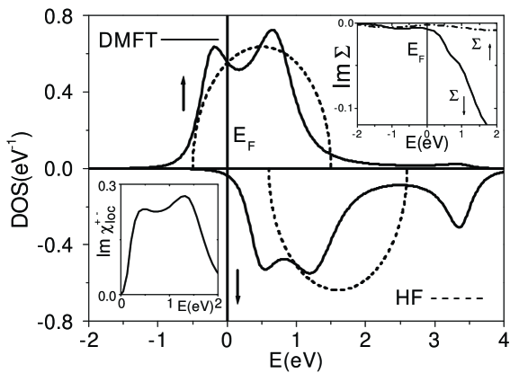
Figure 13: Density of states for HMF in the Hartree-Fock (HF) approximation (dashed line) and in QMC solution of DMFT problem for semi-circular model (solid line) with the band-width $W$=2 eV,Coulomb interaction $U$=2 eV, $\Delta$=0.5 eV, chemical potential $\mu$=-1.5 eV and temperature $T$=0.25 eV. Insets: imaginary part of the the spin-flip susceptibility (left) and imaginary part of selfenergy (right).Chioncel et al. (2003a)

The left inset of Fig. 13, represents the imaginary part of the local spin-flip susceptibility. One can see a well pronounced shoulder ($\simeq 0.5$ eV), which is related to a characteristic magnon excitation Irkhin and Katsnelson (1985b); Irkhin and Katsnelson (1994, 1990). There is a broad maximum at about $1$ eV, which corresponds to the Stoner excitation energy. The right inset of Fig. 13, represents the imaginary part of self-energy. The spin-up channel can be described by a Fermi-liquid type behavior with a parabolic energy dependence $-\mathrm{Im}\Sigma^{\uparrow}\propto(E-E_{F})^{2}$, whereas in the spin down channel the NQP shoulder at 0.5 eV is visible. Due to the relatively high temperature ($T=0.25$ eV) in the QMC calculation the NQP tail extends below the Fermi level (remember that at zero temperature the tail should vanish exactly at the Fermi level, Sect.III.2).

IV.3 Spin-polarized T-matrix fluctuating exchange approximation

Most of HMF materials are moderately or weakly correlated systems. This means that one can use some perturbative approaches which make computations much less expensive and allow one to work with the complete four-index Coulomb interaction matrix. A very efficient perturbative scheme has been proposed by Bickers and Scalapino Bickers and Scalapino (1989) and was called fluctuating exchange approximation (FLEX). This was generalized to the multiband case and used in the context of the DMFT in Lichtenstein and Katsnelson (1998); Katsnelson and Lichtenstein (1999). The latter step means that this approach is used not directly for the whole crystal, but for the effective impurity problem, so that the momentum dependence of the Green’s functions is neglected. On the other hand, self-consistency of the DMFT procedure makes the description of the local effects in perturbative schemes more accurate. For example, in the case of one-band half-filled Hubbard model the second-order perturbation expression for the self-energy in the context of the DMFT provides correct atomic limit and, actually, very accurate description of the metal-insulator transition Kajueter and Kotliar (1996). A starting point in the FLEX approximation is the separation of different interaction channels. The symmetrization of bare U matrix is done over particle-hole and particle-particle channels:

$$U_{m_{1}m_{1}^{\prime}m_{2}m_{2}^{\prime}}^{d} = 2U_{m_{1}m_{2}m_{1}^{\prime}m_{2}^{\prime}}^{i}-U_{m_{1}m_{2}m_{2}^{\prime}m_{1}^{\prime}}^{i}$$

$$U_{m_{1}m_{1}^{\prime}m_{2}m_{2}^{\prime}}^{m} = -U_{m_{1}m_{2}m_{2}^{\prime}m_{1}^{\prime}}^{i}$$

$$U_{m_{1}m_{1}^{\prime}m_{2}m_{2}^{\prime}}^{s} = \frac{1}{2}(U_{m_{1}m_{1}^{\prime}m_{2}m_{2}^{\prime}}^{i}+U_{m_{1}m_{1}^{\prime}m_{2}^{\prime}m_{2}}^{i})$$

$$U_{m_{1}m_{1}^{\prime}m_{2}^{\prime}m_{2}}^{t} = \frac{1}{2}(U_{m_{1}m_{1}^{\prime}m_{2}^{\prime}m_{2}}^{i}-U_{m_{1}m_{1}^{\prime}m_{2}m_{2}^{\prime}}^{i})$$ (176)

The above expressions are the matrix elements of bare interaction which can be obtained with the help of the pair operators corresponding to different channels:

• particle-hole density

  $$d_{12}=\frac{1}{\sqrt{2}}(c_{1\uparrow}^{+}c_{2\uparrow}+c_{1\downarrow}^{+}c_{2\downarrow})$$ (177)

• particle-hole magnetic

  $$m_{12}^{0} = \frac{1}{\sqrt{2}}(c_{1\uparrow}^{+}c_{2\uparrow}-c_{1\downarrow}^{+}c_{2\downarrow})$$

  $$m_{12}^{+} = c_{1\uparrow}^{+}c_{2\downarrow}$$ (178)

  $$m_{12}^{+} = c_{1\downarrow}^{+}c_{2\uparrow}$$

• particle-particle singlet

  $$s_{12} = \frac{1}{\sqrt{2}}(c_{1\downarrow}c_{2\uparrow}-c_{1\uparrow}c_{2\downarrow})$$

  $$s_{12}^{+} = \frac{1}{\sqrt{2}}(c_{1\downarrow}^{+}c_{2\uparrow}^{+}-c_{1\uparrow}^{+}c_{2\downarrow}^{+})$$ (179)

• particle-particle triplet

  $$t_{12}^{0} = \frac{1}{\sqrt{2}}(c_{1\downarrow}c_{2\uparrow}-c_{1\uparrow}c_{2\downarrow})$$

  $$t_{12}^{+0} = \frac{1}{\sqrt{2}}(c_{1\downarrow}^{+}c_{2\uparrow}^{+}-c_{1\uparrow}^{+}c_{2\downarrow}^{+})$$

  $$t_{12}^{\pm} = c_{1\uparrow,\downarrow}c_{2\downarrow,\uparrow}$$

  $$t_{12}^{\pm} = c_{1\uparrow,\downarrow}^{+}c_{2\downarrow,\uparrow}^{+}$$ (180)

  These operators describe the correlated movements of the electrons and holes below and above the Fermi level and therefore play an important role in defining the spin dependent effective potentials $W_{m_{1}m_{2}m_{3}m_{4}}^{\sigma\sigma^{\prime}}$.

In the spin polarized $\mathit{T}$-matrix fluctuating exchange approximation (SPTF) scheme Katsnelson and Lichtenstein (2002) the particle-particle interactions are described in the $T$-matrix approach Galitski (1958); Kanamori (1963) where for the effective interaction the sum over the ladder graphs are carried out with the aid of the so called $T-$matrix which obeys the Bethe–Salpether-like integral equation:

$$\langle 13|T^{\sigma\sigma^{\prime}}(i\Omega)|24\rangle = \langle 13|v|24\rangle$$ (181)

$$- \frac{1}{\beta}\sum_{\omega}\sum_{5678}G_{56}^{i\sigma}(i\omega)G_{78}^{i\sigma^{\prime}}(i\omega)G(i\Omega-i\omega)\langle 68|T^{\sigma\sigma^{\prime}}(i\Omega)|24\rangle$$

The corresponding contributions to the self-energy is described by the Hartree and Fock diagrams with the formal replacement of the bare interaction by the $T-$matrix:

$$\Sigma_{12,\sigma}^{(TH)}(i\omega) = \frac{1}{\beta}\sum_{\Omega}\sum_{34\sigma^{\prime}}\langle 13|T^{\sigma\sigma^{\prime}}(i\Omega)|24\rangle G_{43}^{\sigma^{\prime}}(i\Omega-i\omega)$$ (182)

$$\Sigma_{12,\sigma}^{(TF)}(i\omega) = -\frac{1}{\beta}\sum_{\Omega}\sum_{34\sigma^{\prime}}\langle 14|T^{\sigma\sigma}(i\Omega)|32\rangle G_{34}^{i\sigma}(i\Omega-i\omega)$$ (183)

The “Hartree” contribution dominates for small concentration of electrons and holes; these two contributions together contain all second-order in $V$ terms in the self-energy.

Combining the density and magnetic parts of the particle-hole channel we can write down the expression for the interaction part of the Hamiltonian Lichtenstein and Katsnelson (1998); Katsnelson and Lichtenstein (1999).

$$\mathcal{H}_{U}=D\ast H^{U}\ast D^{+}$$

$$\mathcal{H}_{U}=\frac{1}{2}\mathrm{Tr}(D^{+}\ast V^{\|}\ast D+m^{+}\ast V_{m}^{\bot}\ast m^{-}+m^{-}\ast V_{m}^{\bot}\ast m^{+})$$ (184)

where $D$ is a row vector with elements $(d,m^{0})$, and $D^{+}$ is a column vector with elements $(d^{+}m_{0}^{+})$, $\ast$ stands for the matrix multiplication with respect to the pairs of orbital indices. It follows from the model consideration presented above that for proper describing the effects of electron-magnon interactions it is important to replace the bare spin-flip potential by a static limit of the T-matrix (see Eqs.(6) and (34)). With this replacement, the expression of the effective potential is:

$$V^{\|}(i\omega) = \frac{1}{2}\left(\begin{array}[]{cc}V^{dd}&V^{dm}\\ V^{md}&V^{mm}\end{array}\right)$$ (187)

$$(V_{m}^{\bot})_{1234} = \langle 13|T^{\uparrow\downarrow}|42\rangle$$ (188)

The matrix elements of the effective interaction for $z$ (longitudinal) spin fluctuations are:

$$V_{dd} = \frac{1}{2}\sum_{\sigma}(\sum_{\sigma^{\prime}}\langle 13|T^{\sigma\sigma^{\prime}}|42\rangle-\langle 13|T^{\sigma^{\prime}\sigma^{\prime}}|42\rangle)$$

$$V_{dm}=V_{md} = \frac{1}{2}\sum_{\sigma\sigma^{\prime}}\sigma(\langle 13|T^{\sigma\sigma}|42\rangle-\langle 13|T^{\sigma\sigma}|24\rangle+\langle 13|T^{\sigma^{\prime}\sigma}|42\rangle)$$

$$V_{mm} = \frac{1}{2}\sum_{\sigma}(\sum_{\sigma^{\prime}}\sigma\sigma^{\prime}\langle 13|T^{\sigma\sigma^{\prime}}|42\rangle-\langle 13|T^{\sigma^{\prime}\sigma^{\prime}}|42\rangle)$$ (189)

Further we introduce the expressions for the generalized longitudinal ($\chi^{\|}$) and transverse ($\chi^{\bot}$) susceptibilities

$$\chi^{\bot}(i\omega) = [1+V_{m}^{\bot}\Gamma^{\uparrow\downarrow}(i\omega)]^{-1}\ast\Gamma^{\uparrow\downarrow}(i\omega)$$ (190)

$$\chi^{\|}(i\omega) = [1+V^{\|}\ast\chi_{0}^{\|}(i\omega)]^{-1}\ast\chi_{0}^{\|}(i\omega)$$ (191)

where $\Gamma(i\omega)$ is the Fourier transform of the empty loop:

$$\Gamma_{m_{1}m_{2}m_{3}m_{4}}^{\sigma\sigma^{\prime}}(\tau)=-G_{m_{2}m_{3}}^{i\sigma}(\tau)G_{m_{4}m_{1}}^{i\sigma}(-\tau)$$ (192)

and the bare matrix longitudinal susceptibility is:

$$\chi_{0}^{\|}(i\omega)=\frac{1}{2}\left(\begin{array}[]{cc}{\Gamma}^{\uparrow\uparrow}+{\Gamma}^{\downarrow\downarrow}&{\Gamma}^{\uparrow\uparrow}-{\Gamma}^{\downarrow\downarrow}\\ {\Gamma}^{\uparrow\uparrow}-{\Gamma}^{\downarrow\downarrow}&{\Gamma}^{\uparrow\uparrow}+{\Gamma}^{\downarrow\downarrow}\end{array}\right)$$ (193)

The four matrix elements correspond to the density-density $(dd)$, density-magnetic $(dm^{0})$, magnetic-density $(m^{0}d)$ and magnetic-magnetic channels $(m^{0}m^{0})$ and couple longitudinal magnetic fluctuation with density magnetic fluctuation. In this case the particle hole contribution to the self-energy is:

$$\Sigma_{12\sigma}^{(ph)}(\tau)=\sum_{34\sigma^{\prime}}W_{1342}^{\sigma\sigma^{\prime}}(\tau)G_{34}^{\sigma^{\prime}}$$ (194)

with the particle-hole fluctuation potential matrix

$$W^{\sigma\sigma^{\prime}}(i\omega)=\left(\begin{array}[]{cc}{W}_{\uparrow\uparrow}&{W}_{\uparrow\downarrow}\\ {W}_{\downarrow\uparrow}&{W}_{\downarrow\downarrow}\end{array}\right)$$ (195)

and the spin-dependent effective potentials are defined by

$$W_{\uparrow\uparrow} = \frac{1}{2}V^{\|}\ast(\chi^{\|}-\chi_{0}^{\|})\ast V^{\|}$$

$$W_{\downarrow\downarrow} = \frac{1}{2}V^{\|}\ast(\tilde{\chi}^{\|}-\tilde{\chi}_{0}^{\|})\ast V^{\|}$$

$$W_{\uparrow\downarrow} = \frac{1}{2}V_{m}^{\bot}\ast(\chi^{+-}-\chi_{0}^{+-})\ast V_{m}^{\bot}$$

$$W_{\downarrow\uparrow} = \frac{1}{2}V_{m}^{\bot}\ast(\chi^{-+}-\chi_{0}^{-+})\ast V_{m}^{\bot}$$ (196)

where $\tilde{\chi}^{\|},\tilde{\chi}_{0}^{\|}$ differ from the values of $\chi^{\|},\chi_{0}^{\|}$ by the replacement $\Gamma^{\uparrow\uparrow}\leftrightarrow\Gamma^{\downarrow\downarrow}$ in equation (193). The final expression for the SPTF self-energy is given by:

$$\Sigma=\Sigma^{(TH)}+\Sigma^{(TF)}+\Sigma^{(ph)}$$ (197)

Due to off-diagonal spin structure of the self-energy $\Sigma^{(ph)}$ this method can be used to consider the non-quasiparticle states in HMF. A more detailed justification and description of the method is presented in Katsnelson and Lichtenstein (2002). This approach was also generalized to the case of strong spin-orbit coupling and used for actinide magnets Pourovskii et al. (2006, 2005). In that case separation into density and magnetic channels is not possible and one should work with the $4\times 4$ supermatrices for the effective interaction.

Recently several LDA+DMFT calculations of different HMF materials have been carried out. Now we review briefly the results of these calculations focusing mainly on non-quasiparticle states resulting from the electron-magnon interactions. LDA+DMFT is the only contemporary practical way to consider them in the electronic structure calculations.

V Electronic structure of specific half-metallic compounds

V.1 Heusler alloys.

V.1.1 NiMnSb: electronic structure and correlations

The intermetallic compound NiMnSb crystallizes in the cubic structure of MgAgAs type (C1_b) with the $fcc$ Bravais lattice (space group $F\overline{4}3m=T_{d}^{2}$). The crystal structure is shown in Fig. 14. This structure can be described as three interpenetrating fcc lattices of Ni, Mn and Sb. A detailed description of the band structure of semi-Heusler alloys was given by using electronic structure calculations analysis  de Groot et al. (1983b), Öğüt and Rabe (1995); Galanakis et al. (2002a); Nanda and Dasgupta (2003); Kulatov and Mazin (2003); Galanakis and Mavropoulos (2007); we briefly summarize the results.

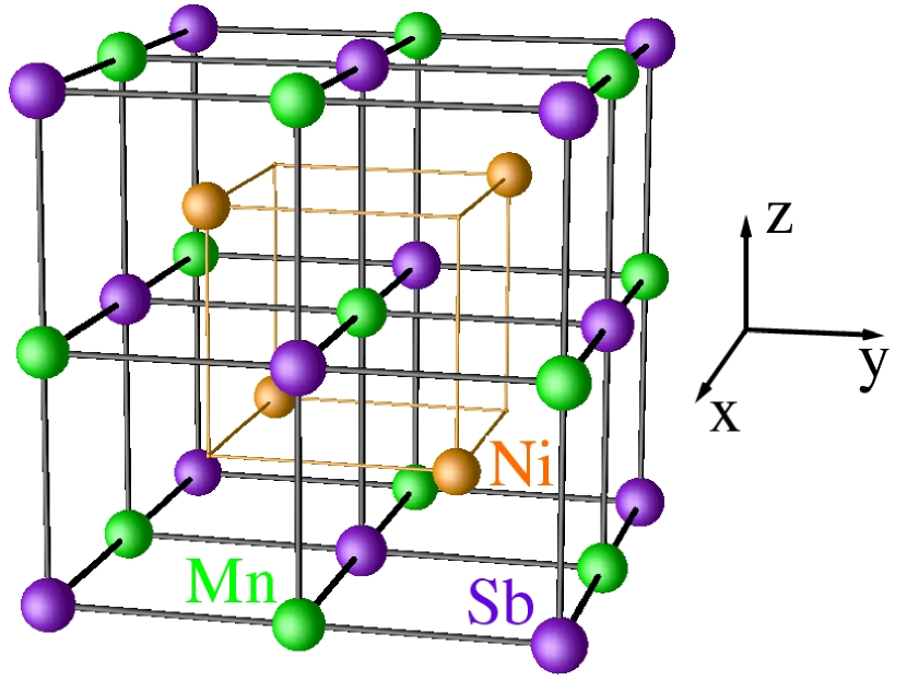
Figure 14: (Color online) C1_b structure with the fcc Bravais lattice (space group $F\overline{4}3m$). Mn (green) and Sb (purple) atoms are located at (0, 0, 0) and ($\frac{1}{2}$, $\frac{1}{2}$, $\frac{1}{2}$) forming the rock salt structure arrangement. Ni (orange) atom is located in the octahedrally coordinated pocket, at one of the cube center positions ($\frac{3}{4}$, $\frac{3}{4}$, $\frac{3}{4}$) leaving the other ($\frac{1}{4}$, $\frac{1}{4}$, $\frac{1}{4}$) empty. This creates voids in the structure. Yamasaki et al. (2006)

To obtain the minority spin gap, not only the Mn$-d$–Sb$-p$ interactions, but also Mn$-d$–Ni$-d$ interactions are to be taken into account. Moreover, the loss of inversion symmetry produced by C1_b structure (the symmetry lowering from $O_{h}$ in the L2₁ structure to $T_{d}$ in the C1_b structure at Mn site) is an essential additional ingredient. All the above interactions combined with the $T_{d}$ symmetry lead to a nonzero anticrossing of bands and to gap opening.

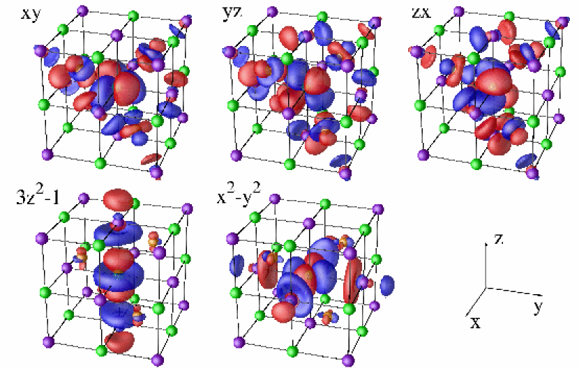
Figure 15: (Color online) NMTO Mn-$d$ Wannier orbitals of NiMnSb. Ni is orange, Mn is green, and Sb is purple. Red/blue indicates a positive/negative sign. Upper panel: $t_{2g}$ orbitals; $d_{xy}$ (left), $d_{yz}$ (middle), $d_{zx}$ (right). The triply-degenerate $t_{2g}$ orbitals can be obtained by the permutation of axes. Lower panel: $e_{g}$ orbitals; $d_{3z^{2}-1}$ (left), $d_{x^{2}-y^{2}}$ (middle). These $e_{g}$ orbitals are doubly degenerated.Yamasaki et al. (2006)

The large exchange splitting of Mn atom (producing the local Mn magnetic moment of about 3.7 $\mu_{B}$) is crucial to induce a half-metallic structure. In the spin-polarized calculation the position of $t_{2g}$ and $e_{g}$ Ni states is changed slightly, so that the exchange splitting on Ni is not large. The local Ni magnetic moment calculation gives a value around 0.3$\mu_{B}$.

Figure 16: Full basis set spin-polarized (ferromagnetic) bands for NiMnSb; majority spin (left) and minority spin (right). The high-symmetry points are; $W(\frac{1}{2},1,0)$, $L(\frac{1}{2},\frac{1}{2},\frac{1}{2})$, $\Gamma(0,0,0)$, $X(0,1,0)$, $K(\frac{3}{4},\frac{3}{4},0)$, in $W$–$L$–$\Gamma$–$X$–$W$–$K$–$\Gamma$ line, and $X(0,0,1)$, $U(\frac{1}{4},\frac{1}{4},1)$, $L(\frac{1}{2},\frac{1}{2},\frac{1}{2})$, in $X$–$U$–$L$ line.Yamasaki et al. (2006)

The non-spin-polarized result has a striking resemblance to the majority spin-polarized calculations, presented in Fig. 16. Kulatov et al. explained half-metallicity of NiMnSb by the extended Stoner factor calculations in the rigid-band approximation  Kulatov and Mazin (2003): the minority spin-band gap opens due to the exchange splitting which shifts minority bands, so that they become empty.

There is an excellent agreement between the first band-structure calculation  de Groot et al. (1983b) and recent N-th order muffin-tin orbitals (NMTO) investigations Yamasaki et al. (2006); Andersen and Saha-Dasgupta (2000); Zurek et al. (2005). NMTO Wannier Mn $d$ orbitals are shown in Fig. 15. The triple-degenerate manganese $t_{2g}$ orbitals are very complicated due to the hybridization with Ni $d$ and Sb $p~{}$states. The $d_{xy}$ orbital at Mn site is deformed by antibonding with Ni $d~{}$state directed tetrahedrally to [$11\bar{1}$], [$\bar{1}\bar{1}\bar{1}$], [$1\bar{1}1$], and [$\bar{1}11$]. The same Ni $d~{}$orbitals couple with Sb $p$ states. The direct Mn-$d_{xy}$–Sb-$p$ $\pi$ coupling is not seen since the distance is $d$(Mn–Sb):$d$(Ni–Sb) $=1:\sqrt{3}/2$. Therefore the Ni-$d$–Sb-$p$ interactions are more favorable. The dispersion of the Mn $t_{2g}~{}$bands is mainly due to hopping via the tails of Sb $p$ and Ni $d~{}$orbitals. On the other hand, the next-nearest neighbor (n.n.n.) $d-d$ hopping of $t_{2g}$ orbital is small. The $e_{g}$ orbitals at Mn site are much easier to understand: they point towards Sb atoms, and a strong $pd\sigma$ coupling between Sb $p$ and Mn e${}_{g}~{}$states is seen. This induces large n.n.n. $d$-$d$ hoppings.

The Wannier orbital analysis for NiMnSb Yamasaki et al. (2006) confirms the previous conclusions of Ref.de Groot et al. (1983b) about the role of $p$-$d$ hybridization as well as the role of $d$-$d$ hybridizationGalanakis et al. (2002a). The LDA partial density of states for half-metallic NiMnSb and the fat-band structure which marks the main orbital character of valence states are presented in the Fig. 17,18, 19. One can see that the spin-up Mn $d$ and Ni $d$ states are located at the same energy region, while spin-down bands are separate due to the significant Mn exchange splitting. The top of the valence spin-down bands form by the Mn $t_{2g}$, Sb $p$ and Ni $t_{2g}$ orbitals, while bottom of the conduction bands are due to the Mn $e_{g}$ and $t_{2g}$ states. This means that large Mn spin-splitting and Sb mediated indirect Mn-Ni interactions are responsible for formation of the half-metallic gap. One can see this complicated Mn $t_{2g}$ valence orbitals with large contributions of Sb $p$ and Ni $t_{2g}$ states in the Fig. (15). The physical picture of the downfolding analysis should not change very much if one explicitly includes Sb $p$ and Ni $d$ orbitals.

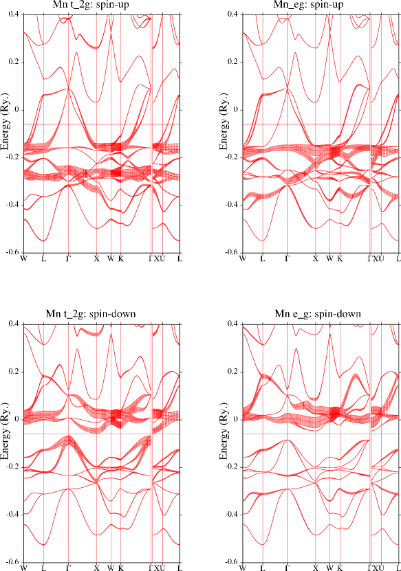
Figure 17: Decorated (fat) bands for the spin-polarized (ferromagnetic) NiMnSb; Mn majority spin (up) and minority spin (down). The high-symmetry points are; $W(\frac{1}{2},1,0)$, $L(\frac{1}{2},\frac{1}{2},\frac{1}{2})$, $\Gamma(0,0,0)$, $X(0,1,0)$, $K(\frac{3}{4},\frac{3}{4},0)$, in $W$–$L$–$\Gamma$–$X$–$W$–$K$–$\Gamma$ line, and $X(0,0,1)$, $U(\frac{1}{4},\frac{1}{4},1)$, $L(\frac{1}{2},\frac{1}{2},\frac{1}{2})$, in $X$–$U$–$L$ line Yamasaki (2006).

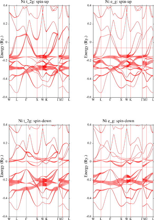
Figure 18: Decorated (fat) bands for the spin-polarized (ferromagnetic) NiMnSb; Ni majority spin (up) and minority spin (down) Yamasaki (2006).

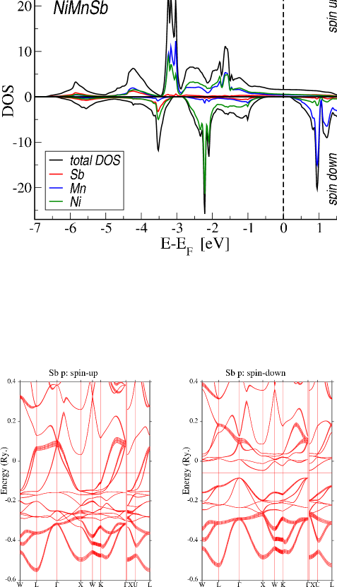
Figure 19: Upper figure: FLAPW calculation of spin-polarized NiMnSb Lezaic (2006). Lower figures: Decorated (fat) bands for the spin-polarized (ferromagnetic) NiMnSb; Sb majority spin (up) and minority spin (down) Yamasaki (2006).

We discuss now in detail the prototype half-metallic ferromagnet NiMnSb where the gap is situated in the spin-down (minority) channel. The temperature dependence of the HMF electronic structure and stability of half-metallicity against different spin-excitations are crucial for practical applications in spintronics. A simple attempt to incorporate finite-temperature effects Skomski and Dowben (2002); Dowben and Skomski (2003), leading to static non-collinear spin-configurations, shows a mixture of spin up and spin down density of states that destroy the half-metallic behavior. In Ref. Chioncel et al. (2003a) a different more natural approach was used to investigate the proper effect of dynamical spin fluctuations on the electronic structure at $T<T_{C}$, within the half-metallic ferromagnetic state.

The LDA+DMFT calculation for NiMnSb Chioncel et al. (2003a) was the first application of the combined electronic structure and many-body technique to HMF. Aryasetiawan et al pointed out recently Aryasetiawan et al. (2004) that a rigorous way to define the screened frequency-dependent on-site Coulomb interactions matrix elements for correlated states related with generalized GW scheme where $d-d$ screening is suppressed to preserve the double counting of in the model approach. However, in practice for realistic materials, the elimination of degrees of freedom is a very difficult procedure. To find the average Coulomb interaction on the $d$ atoms $U$ and corresponding exchange interactions $J$, a more simple approach, the constrained LDA scheme  Dederichs et al. (1984); Norman and Freeman (1986); McMahan et al. (1988); Gunnarsson et al. (1989); Hybertsen et al. (1989); Anisimov and Gunnarsson (1991), can be used. In this approach the Hubbard $U$ is calculated from the variation of the total energy with respect to the occupation number of the localized orbitals. In such a scheme, the metallic screening is rather inefficient for 3$d$ transition metals, and effective $U$ is of the order of 6 eV Anisimov and Gunnarsson (1991). The perfect metallic screening will lead to a smaller value of $U$. Unfortunately, there are no reliable scheme to calculate $U$ within constrained LDA for metals Solovyev and Imada (2005), and in the works  Chioncel et al. (2003a); Chioncel et al. (2005); Chioncel et al. (2006a, b) some intermediate values were chosen, $U=2\div 4$ eV and $J=0.9$ eV. The recent analysis of angle-resolved photoemission and the LDA theory indicates a shift of spectral function of the order of $0.5\div 1$ eV, which can be attributed to correlation effects beyond LDA Correa et al. (2006). First angle-resolved photoemission results Kisker et al. (1987) in generally agree with the LDA band structure, but demonstrate the same shift of quasiparticle dispersion of the order of $0.5$ eV below the Fermi level for spin-down Mn $t_{2g}$ bands. This can easily lead to the effective Hubbard interactions in the static mean-field approximation of the order of $U^{\ast}=1$ eV, although one should carefully investigate the effects of spin-orbital splitting. Since the spherically-average effective Hubbard interactions is equal to $U^{\ast}=U-J$ and the value of intra-atomic exchange interactions is not screened much in solids being of the order of $J=1$ eV, we can conclude from the photoemission experiments Kisker et al. (1987) and resonant x-ray scattering Yablonskikh et al. (2001) that the Hubbard interactions $U=2$ eV is quite reasonable. An account of the correlation effects in the framework of the LDA+DMFT method also improves the description of magnetooptical properties of NiMnSb Chadov et al. (2006).

The typical results for density of states using LDA and LDA+DMFT is presented in Fig. 20. The LDA+DMFT density of states shows the existence of non-quasiparticle states in the LDA gap of the spin down channel just above the Fermi level.

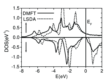
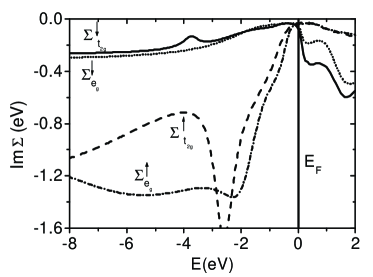
Figure 20: Density of states for HMF NiMnSb in LSDA scheme (dashed line) and in LDA+DMFT scheme (solid line) with effective Coulomb interaction $U$=3 eV, exchange parameter $J$=0.9 eV and temperature $T$=300 K. The non-quasiparticle state is evidenced just above the Fermi level. The imaginary part of self-energies ${\rm Im}\Sigma_{d}^{\downarrow}$ for $t_{2g}$ (solid line) and $e_{g}$ (dotted line), ${\rm Im}\Sigma_{d}^{\uparrow}$ for $t_{2g}$ (dashed line) and $e_{g}$ (dashed dotted line) respectively.

It is important to mention that the magnetic moment per formula unit is not sensitive to the $U$ values. For a temperature $T=300$ K the calculated magnetic moment, $\mu=3.96\mu_{B}$, is close to the zero-temperature LDA-value which is integer, $\mu=4$ $\mu_{B}$. This means that the half-metallic state is stable with respect to switching on the correlation effects. The DMFT gap in the spin down channel, defined as the distance between the occupied part and starting point of NQP tail, is also not very sensitive to $U$. The total DOS is also weakly $U$-dependent due to the $T$-matrix renormalization effects.

In comparison with the LDA result, a strong spectral weight transfer is present for the unoccupied part of the band structure due to appearance of the non-quasiparticle states in the energy gap above the Fermi energy (Sect.III.2). Their spectral weight is not too small and has a relatively weak dependence on the $U$ value (Fig. 21), which is also a consequence of the $T$-matrix renormalization Katsnelson and Lichtenstein (2002).

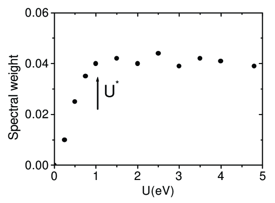
Figure 21: Spectral weight of the non-quasiparticle state, calculated as a function of average on-site Coulomb repulsion $U$ at temperature $T$=300 K.Chioncel et al. (2003a)

For spin-up states we have a normal Fermi-liquid behavior $-\mathrm{Im}\Sigma_{d}^{\uparrow}(E)\propto(E-E_{F})^{2}$ with a typical energy scale of the order of several eV. The spin-down self energy behaves in a similar way below the Fermi energy, with a bit smaller energy scale. At the same time, a significant increase in $\mathrm{Im}\Sigma_{d}^{\downarrow}(E)$ with a much smaller energy scale (tenths of eV) is observed right above the Fermi level, which is more pronounced for $t_{2g}$ states (Fig. 20). The NQP states are visible in the spin-down DOS, Fig. 20, at the same energy scale as the imaginary part of $\Sigma^{\downarrow}$. A similar behavior is evidenced in the model calculation of Fig. 13. The NQP spectral weight in the density of states (Fig. 20) is proportional to the imaginary part of the self-energy.

From the general many-body theory, the DMFT approach is neglecting the momentum dependence of the electron self-energy. In many cases, such as the Kondo effect and the Mott metal-insulator transition the energy dependence of the self-energy is obviously more important than the momentum dependence and, therefore, the DMFT scheme is adequate to consider these problems Georges et al. (1996). In the case of itinerant electron ferromagnetism, the situation is much less clear. However, the LDA+DMFT treatment of finite temperature magnetism and electronic structure in Fe and Ni appeared to be quite successful Lichtenstein et al. (2001). Experimentally, even in itinerant electron paramagnets which are close to ferromagnetic instability, such as Pd, the momentum dependence of the self-energy does not seem to be essential Joss et al. (1984). One can expect that in magnets with well defined local moments such as half-metallic ferromagnets the local DMFT approximation for the self-energy should be even more accurate. In particular, as discussed above, it can be used for the calculations of spin-polaronic or non-quasiparticle effects in these materials.

V.1.2 Impurities in HMF: lanthanides in NiMnSb

Here we discuss the introduction of non-intrinsic deffects in NiMnSb, which preserves the half-metallic properties on one hand while optimizing the magnetic disorder on the other hand Attema et al. (2004). Good candidates are the rare-earth impurities in NiMnSb Attema et al. (2004); Chioncel (2004). The motivation of this choice is connected with the substantial spin-orbit interaction in the rare-earth localized $f$ shell. Besides that, the origin of the band gap in NiMnSb is closely related to the band gap in III-V semiconductors: it is expected that a substitution of some of the tetravalent element in NiMnSb by a lanthanide preserves the essential feature of the half-metal: the band gap for one spin direction.

These systems can be really synthesized, compounds RNiSb (for heavy rare earths R) existing with exactly the same crystal structure as NiMnSb. The rare-earth atoms which show both a large spin and orbital moment can be expected to introduce a large spin-orbit interaction, in other words around 1/4 (Nd) and 3/4 (Er) in the lanthanides series. Total energy calculations allow one to evaluate the coupling between the rare-earth ($4f$) impurity spins and the manganese ($3d$) conduction electron spins. For a substantial coupling the fluctuations of the Mn ($3d$) conduction electron spins, i.e. the spin wave, might be blocked, thus the magnon branch is qualitatively changed. In contrast with the clean limit (pure NiMnSb), the magnon spectra of NiMn_1-xR_xSb present a fragmented structure with several gaps in the Brillouin zone. This fragmentation implies that the finite temperature effects are diminished for a suitably chosen rare-earth.

The ab-initio electronic structure calculations were carried out using the scalar relativistic linear muffin-tin orbital (LMTO) method within the atomic-sphere approximation in two flavors: LDA and LDA$+U$ Anisimov et al. (1997a); Andersen (1975); Andersen and Jepsen (1984). To evaluate the coupling between the rare-earth and the Mn sublattices, ferro- and ferrimagnetic structures were taken as the initial state of the calculation and they were preserved after the self-consistent calculation.

A simplified model was used that captures the complex interplay of the Mn ($3d$) itinerant conduction band electrons and the localized $4f$ electrons, the latter carrying a strong magnetic moment. This model deals with a mean-field decoupling, in which the Mn $3d$ and the R $f$ states are described by the LDA$+U$ whereas the $3d-4f$ interaction is treated as perturbation. The corresponding mean-field Hamiltonian can be written in the form:

$$\mathcal{H}\simeq\mathcal{H}_{\mathrm{LDA+U}}-J\sum_{i}\sigma_{i}^{3d}S_{i+\delta}^{f}$$ (198)

where the spin of the conduction electron at site $R_{i}$ is denoted by $\sigma_{i}^{3d}$ and $S_{i+\delta}^{f}$ represents the spin of the 4f shell at the $R_{i+\delta}$ site. The Mn $d$ local moment fluctuations could be quenched by a strong $f-d$ coupling, which affects the magnon excitations. The strength of such a coupling was evaluated by calculating in an ab-initio fashion the total energy of NiMn_1-xR_xSb compounds for a parallel/antiparallel $f-d$ coupling Chioncel (2004); Attema et al. (2004). Given the geometry of the cell the lanthanide substitution is realized in the $fcc$-Mn sublattice, so 12 pairs of R($4f$)-Mn($3d$) are formed. The $f-d$ coupling is calculated as the $E_{\uparrow\uparrow}-E_{\downarrow\uparrow}$ energy corresponding to a pair. Adopting a two sublattices model described by the Hamiltonian (198), i.e. the sublattice of lathanides R($4f$) being antiferro/ferromagnetically oriented with respect to the Mn($3d$) sublattice, the $J$ values correspond to the intersublattice couplings. In pure NiMnSb the ferromagnetic Curie temperature $T_{C}=740$K is determined by the strength of the Mn-Mn ($3d-3d$) sublattice interaction. For a small lanthanide content one can expect that this interaction in NiMn_1-xR_xSb compounds is on the same scale as in pure NiMnSb. Therefore the substitution introduces the competition between the intra- and intersublatice interactions which are crucial parameters for any practical applications. In the case of Nd there is a large $3d-4f$  coupling which should dominate over the $3d-3d$ coupling. For temperatures lower than the Curie temperature corresponding to the Ni₈Mn₇NdSb₈ compound, $T_{C}^{\mathrm{Nd}}$, the $3d-4f$  coupling interaction will lock the Mn ($3d$) magnetic moment fluctuations decreasing the available number of magnon states. Above $T_{C}^{\mathrm{Nd}}$ the thermal fluctuations already took away the long range order of the Mn ($3d$) sublattice, and there are no available magnon states at all. As a consequence, the Nd substitution can be attractive for the high-temperature applications where the $3d-4f$ coupling might play an important role. In the cubic structure of NiMnSb the uniaxial anisotropy is completely missing. Nevertheless, the $4f$ impurity spin-orbit coupling lifts the degeneracy in the $\Gamma$ point. The lowest $3d-4f$ coupling is realized in the case of Ho.

Figure 22: Density of states for the half-metallic ferromagnet Ni₈Mn₇HoSb₈ in the case of anti-parallel $3d-4f$ coupling left, and parallel coupling right.

The LDA$+U$ density of states for HoNi₈Mn₇Sb₈ for $3d-4f$ antiparallel and parallel couplings and $U_{f}=9$ eV value of the on site Coulomb interaction is presented in Fig. (22). On one hand for the antiparallel coupling the magnetic moments are $\mu_{\mathrm{Ho}}^{AF}=-4.09\mu_{B},\mu_{\mathrm{Mn1}}^{AF}=3.73\mu_{B},\mu_{\mathrm{Mn2}}^{AF}=3.80\mu_{B}$ and the gap of $0.55$ eV is situated in the majority spin channel. On the other hand for parallel coupling the magnetic moments have almost the same magnitude $\mu_{\mathrm{Ho}}^{F}=3.96\mu_{B},\mu_{\mathrm{Mn1}}^{F}=3.72\mu_{B},\mu_{\mathrm{Mn2}}^{F}=3.80\mu_{B}$ with a similar gap situated in the minority spin channel. It is important to mention that in the case of $\mathrm{Ni}_{8}\mathrm{Mn}_{7}\mathrm{HoSb}_{8}$ the Ho($4f$) orbitals do not hybridize with the Mn($3d$) orbitals near the Fermi level. As one can see in Fig. (22), the behavior of DOS near the Fermi level is very similar, so that the nature of carriers around $E_{F}$ is not changed.

Figure 23: Density of states of semiconducting HoNiSb.Chioncel (2004)

The electronic structure calculation for the antiferromagnetic HoNiSb compound was performed in Chioncel (2004); Attema et al. (2004). This is known to be a semiconducting material with interesting transport properties (giant magnetoresistance effect Karla et al. (1998b, a); Karla et al. (1999); Pierre and Karla (2000)). The inverse susceptibility curves show a Curie-Weiss behavior down to $10$K Karla et al. (1998b, a); Karla et al. (1999); Pierre and Karla (2000). The onset of the antiferromagnetic ordering was estimated from susceptibility measurements between $1.5$ and $2.5~{}$K, and the neutron diffraction data indicated an antiferromagnetic propagation vector $(1/2,1/2,1/2)$ Karla et al. (1998b, a); Karla et al. (1999); Pierre and Karla (2000). In order to describe the antiferromagnetic ground state, a rhombohedral description of the Ho₂Ni₂Sb₂ unit cell was used. The atoms $\mathrm{Ho}_{1}(0,0,0)$ and $\mathrm{Ho}_{2}(1,1,1)$ acquire magnetic moments of $\mu_{\mathrm{Ho}_{1}}=4.0\mu_{B}$ and $\mu_{\mathrm{Ho}_{2}}^{F}=-4.0\mu_{B},$ respectively. The antiferromagnetic insulating state shows a gap of $0.29$ eV in agreement with the experimental results. There are some qualitative features which are similar for the antiferromagnetic Ho₂Ni₂Sb₂ and the HoNi₈Mn₇Sb₈ compounds: the almost identical magnetic moment $\mu_{\mathrm{Ho}}$ and positions of occupied and unoccupied Ho($4f$) peaks in DOS. Perhaps the most important observation is that the spin-down channel in Ho₂Ni₂Sb₂ is isoelectronic to that in NiMnSb, so that the Ho substitution would preserve the half-metallicity of HoNi₈Mn₇Sb₈ in the minority spin channel.

V.1.3 FeMnSb: a ferrimagnetic half-metal

Early theoretical studies demonstrated that the gap in the minority spin channel is stable with respect to change of the 3d atom X = Fe, Co, Ni in the XMnSb compounds de Groot et al. (1986); Kübler (1984). Noticeable difference between Ni- and Fe-based Heusler alloys is that NiMnSb is a half-metallic ferromagnet with a very small value of Ni magnetic moment ($0.2\mu_{B}$), whereas in FeMnSb the antiferromagnetic coupling between Fe ($-1\mu_{B}$) and Mn ($3\mu_{B}$) moments stabilizes the gap and the half-metallic ferrimagnetic electronic structure de Groot et al. (1986). Unfortunately, the ternary compound FeMnSb does not exist, but indications of its magnetic and crystallographic properties were obtained by extrapolating the series of Ni_1-xFe_xMnSb de Groot et al. (1986) to high Fe concentration.

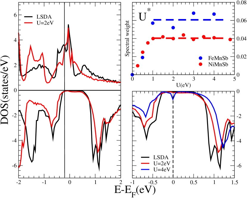
Figure 24: (Color online) Left: Density of states of half-metallic FeMnSb, LSDA (black line) and LSDA+DMFT (red line), for the efective Coulomb interaction $U$=2 eV exchange parameter $J$=0.9 eV and temperature $T$=300 K. Lower right panel: zoom around $E_{F}$ for different values of $U$. Upper right panel: Spectral weight of the NQP states calculated as a function of $U$. The values obtained for NiMnSb Chioncel et al. (2003a) are plotted for comparison.Chioncel et al. (2006a)

In the non-relativistic approximation there are two essentially different sources for states in the gap at finite temperatures. First, there is the simple effect of gap filling due to disorder, i.e. due to scattering on static (classical) spin fluctuation or thermal magnons; this is symmetric with respect to the Fermi energy. On the contrary, the correlation effects result in an asymmetry in the gap filling, spin-down non-quasiparticle states appearing above the Fermi level. One has to take into account also spin-orbit coupling effects mixing the spin-up and spin-down states due to non-zero elements of spin-orbital interactions $V_{SO}^{\sigma,\sigma^{\prime}}$ (see the discussion in Sect.III.2). To illustrate the differences between the static and dynamic effects we plot the DOS of the LDA+DMFT calculations which should be compared with recent results including SO coupling de Groot et al. (1986); Mavropoulos et al. (2004).

A relatively weak dependence of the NQP spectral weight on $U$ (Fig. 24) is evidenced for both NiMnSb and FeMnSb compounds. A “saturation” of the spectral weight for FeMnSb takes place for almost the same value, $U^{\ast}\simeq 1$ eV, as in the case of NiMnSb, which is in agreement with experimental observation of relatively weak correlation effects in Heusler HMF like PtMnSb Kisker et al. (1987). The small value of effective Hubbard parameter can be understood in terms of the large $T$-matrix renormalization of the Coulomb interactions Katsnelson and Lichtenstein (1999, 2002). The spectral weight values for FeMnSb are larger in comparison with those obtained for NiMnSb Chioncel et al. (2003a), which can be attributed to a larger majority spin DOS at the Fermi level.

The spin-orbit coupling produces a peak in the minority-spin channel close to the Fermi level Mavropoulos et al. (2004), which is an order of magnitude smaller than the spectral weight of the NQP states. According to the SO results, the polarization at the Fermi level for NiMnSb and FeMnSb are almost the same. In contrast, the calculation Chioncel et al. (2006a) shows that the spectral weight of the NQP states in FeMnSb is almost twice as large as the value for NiMnSb.

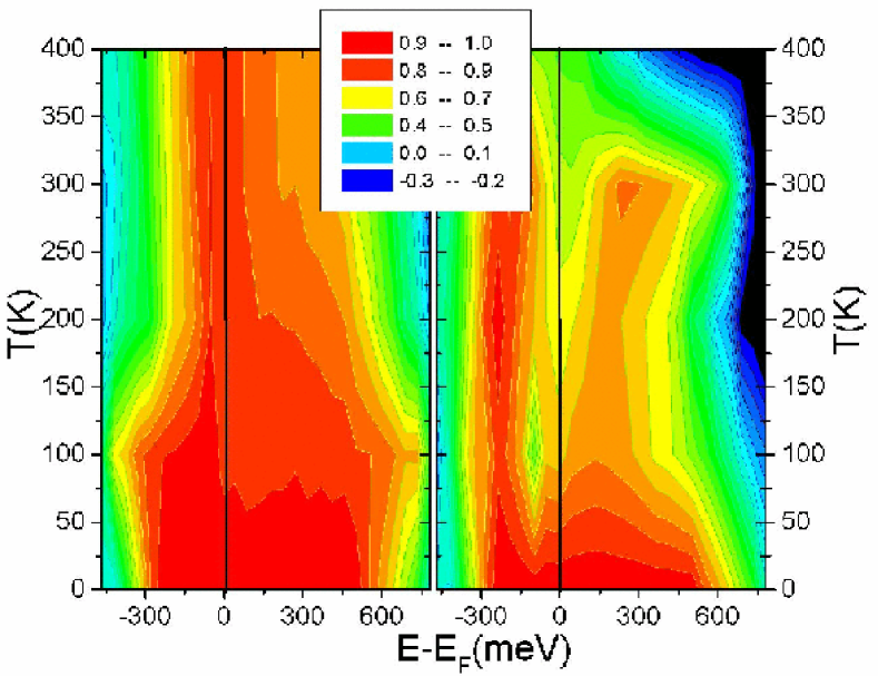
Figure 25: (Color online) Contour plots of polarization as a function of energy and temperature for different values of local Coulomb interaction U. Left $U$=2 eV, right $U$=4 eV. The LSDA polarization is plotted as the $T$=0 K temperature result. The asymmetry of the NQP states, is clearly visible for $U$=4 eV. Chioncel et al. (2006a)

To discuss the influence of temperature and local Coulomb interactions on the polarization in FeMnSb compound, we present results of LDA+DMFT calculations for $T\leq 400~{}\mathrm{K}$ and different $U$’s. Fig.25 presents the contour plot of spin polarization $P(E,T)$ as a function of energy $E$ and temperature $T$ for $U=2$ and 4 eV. The LDA value, plotted for convenience as the $T=0~{}$K result, shows a gap with magnitude $0.8~{}\mathrm{eV,}$ in agreement with previous calculations Mavropoulos et al. (2004).

One can see a peculiar temperature dependence of the spin polarization. The NQP features appear for $E-E_{F}\geq 0$ and are visible in Fig. 24 for $U=2$ eV and $T=300$K. Increasing the value of $U$ from 2 eV to 4 eV, the NQP contribution in depolarization becomes more significant. When the tail of the NQP states crosses the Fermi level, a drastic depolarization at Fermi level takes place, for $U=4$ eV the NQP contribution being pinned to the Fermi level.

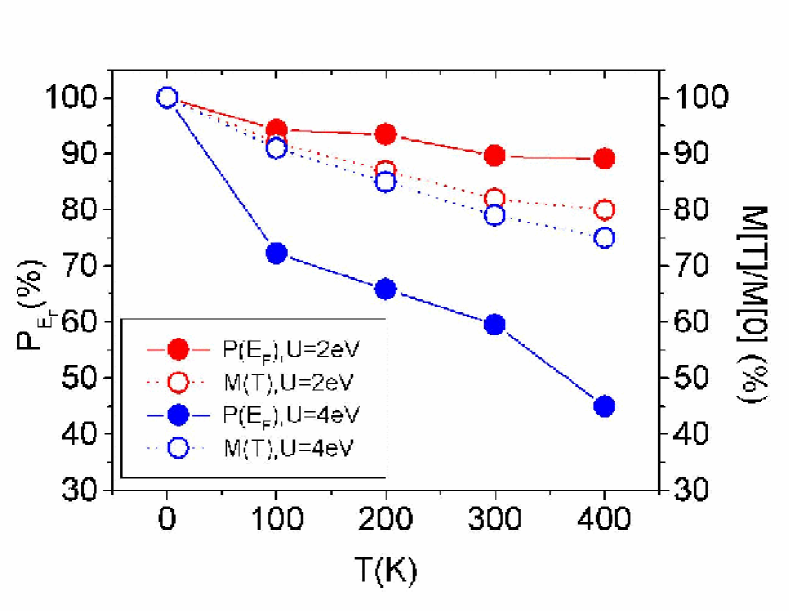
Figure 26: (Color online) Temperature dependent polarization at the Fermi level, $P(E=E_{F},T)$ (solid line) and magnetization (dashed line) for different values of local Coulomb interaction $U$.Chioncel et al. (2006a)

One can see a clear distinction between the finite-temperature behavior of the polarization and magnetization, shown in Fig. 26 for different values of $U$. For $U=4eV$, already at 100K there is a strong depolarization about 25$\%$. On contrary, it is interesting to note that the reduced magnetization $M(T)/M(0)$ decreases slowly in the temperature range shown in Fig. 25. This reduction is a consequence of the finite temperature excitations, i.e. spin-flip processes, affecting both spin channels. In the minority spin channel, NQP states are formed, and in the majority channel a spectral weight redistribution around the Fermi level (Fig.24) contributes to the depolarization. The corresponding depolarization increases with the strength of correlations. The density of NQP states displays a rather strong temperature dependence (Sect.III.3) and results in an asymmetry that is visible in Figs. 24 and 25.

NQP states dominate in the depolarization of this class of Heusler compounds, while spin-orbit contributions are much smaller. In addition, many-body effects are more pronounced in FeMnSb than in NiMnSb. This is connected with the larger DOS in the majority spin channel in the former material. Therefore, doping of NiMnSb by Fe could be an interesting issue to investigate the interplay between alloying and many-body effects. The LDA+DMFT calculations for NiMnSb supercell containing 25 % Fe impurities show a half-metallic character at the LDA level, with the same strong correlation-induced depolarization effects as in pure FeMnSb. Therefore many-body effects for this material are of primary importance even in the presence of disorder. Correlation effects on surfaces of half-metals were discussed recently and it was shown that these states can be probed both directly and via their effect on surface states Irkhin and Katsnelson (2006).

V.1.4 Co₂MnSi: a full-Heusler ferromagnet

The origin of minority band gap in full Heuslers was discussed by Galanakis et al. Galanakis et al. (2006); Galanakis and Mavropoulos (2007). Basing on the analysis of the band structure calculations, it was shown that the $3d$ orbitals of Co atoms from the two different sublattices, Co${}^{1}(0,0,0)$ and Co${}^{2}(1/2,1/2,1/2)$, couple and form bonding hybrids Co¹($t_{2g}$/$e_{g}$) - Co²($t_{2g}$/$e_{g}$). In other words, the $t_{2g}$/$e_{g}$ orbitals of one of the Co atom can couple only with the $t_{2g}$/$e_{g}$ orbitals of other Co atom. Further on, the Co-Co hybrid bonding orbitals hybridize with Mn(d)-$t_{2g}$,$e_{g}$ manifold, while the Co-Co hybrid antibonding orbitals remain uncoupled owing to their symmetry. The Co-Co hybrid antibonding $t_{2g}$ is situated below the Fermi energy $E_{F}$ and the Co-Co hybrid antibonding $e_{g}$ is unoccupied and lies just above the Fermi level. Thus, due to the missing Mn(d)-$t_{2g}$,$e_{g}$ and Co-Co hybrid antibonding hybridization, the Fermi energy is situated within the minority gap formed by the triply degenerate Co-Co antibonding $t_{2g}$ and the double degenerate Co-Co antibonding $e_{g}$.

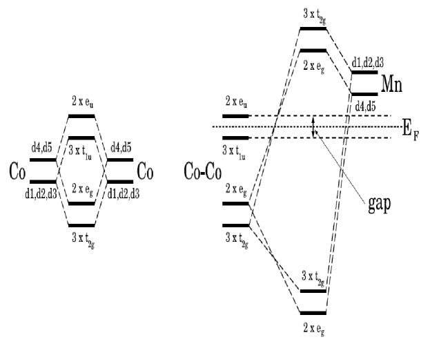
Figure 27: Schematic illustration of the gap formation in Co₂MnZ compounds with Z=Al, Si, Ge,Sn Galanakis et al. (2006).

Fig. 28 shows the results of DOS calculations using the LDA and LDA+DMFT schemes. The inset presents the spin polarization $P(E_{F})=(N_{\uparrow}(E_{F})-N_{\downarrow}(E_{F}))/(N_{\uparrow}(E_{F})+N_{\downarrow}(E_{F}))$. One can see that in the minority spin channel asymmetric NQP states are formed, while in the majority a spectral weight redistribution takes place, which contributes to the depolarization. Contrary to the FeMnSb Chioncel et al. (2006a), where the density of NQP states shows a rather strong temperature dependence, in the full-Heusler Co₂MnSi the temperature dependence is not so significant, similar to the result obtained for NiMnSb Chioncel et al. (2003a).

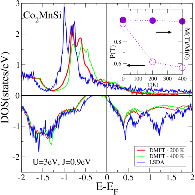
Figure 28: Total density of states of Co₂MnSi full-Heusler alloy. Notice that the gap is formed between the occupied Co-Co antibonding $t_{2g}$ orbitals and empty Co-Co antibonding $e_{g}$ orbitals. The LDA+DMFT results are presented as well for $U=3$eV, and $J=0.9$eV, and different temperatures. The inset shows the finite temperature spin-polarization.

V.2 Half-metallic materials with zinc-blende structure

One of the strongest motivations to investigate magnetic semiconductors and half-metallic ferromagnets is the possibility to design and produce novel stable structures on semiconducting substrates with new interesting properties. From this point of view first-principle studies are an excellent starting point to predict new systems having the desired properties. Using full-potential density-functional method, all the 3d transition metal pnictides and chalcogenides with wurtzite structure were investigated systematically in Ref.Xie et al. (2003a) in order to find half-metallic ferromagnets. These can be fabricated as thin films with thickness large for real spintronic applications. Nine of the wurtzite phases, MnSb, CrAs, CrSb, VAs, VSb, CrSe, CrTe, VSe, and VTe, were found to be robust half-metallic ferromagnets with large half-metallic gaps (0.2$\div$1 eV). Being compatible with the III-V and II-VI semiconductors, these half-metallic ferromagnetic phases, when realized experimentally, would be useful in spintronic and other applications. At the same time, zinc-blende (ZB) phases of MnAs, CrAs and CrSb have been fabricated successfully in the form of nanodots, ultrathin films and multilayers, respectively. A study within density-functional theory Liu (2003) predicted for the ZB CrSb half-metallic ferromagnetism with a magnetic moment of 3.0 $\mu_{B}$ per formula.

V.2.1 CrAs: tunable spin transport

Recently Akinaga et al. Akinaga et al. (2000) found the possibility to fabricate ZB-type CrAs half-metallic ferromagnetic material. Experimental data confirmed that this material is ferromagnetic with the magnetic moment of $3\mu_{B}$, in agreement with theoretical predictions Akinaga et al. (2000). According to this calculation, this half-metallic material has a gap of about 1.8 eV in the minority spin channel, which has attracted much attention to this potential candidate for spintronic applications, keeping in mind also its high Curie temperature $T_{C}$ about $400$K. Recent experiments on CrAs epilayers grown on GaAs$(001)$ evidenced an orthorhombic structure, different from the ZB one, so the structure is rather sensitive to the preparation process Etgens et al. (2004). However, it is highly desirable to explore the possibility of existence of half-metallic ferromagnetism in materials which are compatible with practically important III-V and II-IV semiconductors. For this purpose efforts have been made to investigate metastable ZB structures, such as CrAs Akinaga et al. (2000); Mizuguchi et al. (2002).

It is interesting to explore the mechanisms of half-metallic ferromagnetism at finite temperature from a realistic electronic structure point of view. Theoretical studies Shirai (2003) of the $3d$ transition metal monoarsenides have shown that the ferromagnetic phase of ZB structure CrAs compound should be more stable than the antiferromagnetic one. The many-body effects are very sensitive to structural properties of the artificially produced CrAs compound Chioncel et al. (2005). Similar electronic structure calculations concerning the stability of the half-metallic ferromagnetic state in the ZB structure have been carried out Xie et al. (2003b). The LDA+DMFT calculations were carried out for three lattice constants: the GaAs ($5.65$Å), InAs ($6.06$Å) and the “equilibrium” value ($a_{\mathrm{eq}}=5.8$Å) obtained by density functional calculations Shirai (2003). The corresponding LDA computational results agree with previous ones Akinaga et al. (2000); Shirai (2003); Galanakis and Mavropoulos (2003). In order to evaluate the average Coulomb interaction on the Cr atoms and the corresponding exchange interactions, the constrained LDA method Anisimov and Gunnarsson (1991) was used in Ref Chioncel et al. (2005), which yielded $U=6.5~{}$eV and $J=0.9$ eV. It is important to note that the values of the average Coulomb interaction parameter slightly decrease going from the GaAs ($U=6.6$ eV) to InAs ($U=6.25$ eV) lattice constants, Chioncel et al. (2005) which is in agreement with a naive picture of a less effective screening due to increasing of the distances between the atoms.

The typical insulating screening used in the constraint calculation Anisimov and Gunnarsson (1991) should be replaced by a metallic kind of screening. The metallic screening will lead to a smaller value of $U$. Since there are no reliable schemes to calculate $U$ in metals, some intermediate value were chosen, $U=2$ eV and $J=0.9$ eV. It is important to realize that there are no significant changes in the values of the average Coulomb interaction for the lattice structures studied, the exchange interaction being practically constant. Note that the physical results are not very sensitive to the value of $U$, as it was demonstrated for NiMnSb Chioncel et al. (2003a).

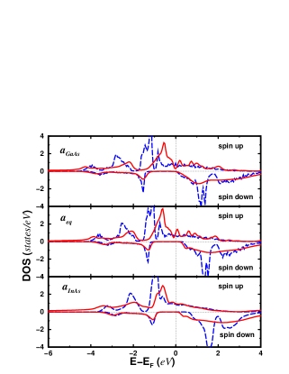
Figure 30: (Color online) Cr density of states calculated in LSDA (dashed line) and LSDA+DMFT (solid line) methods corresponding to a temperature of $T$=200K, average Coulomb interaction parameter $U$=2 eV and exchange $J$=0.9 eV. The non-quasiparticle states are clearly visible for lattice parameters larger than $a_{eq}=5.8\mathring{A}$, in the unoccupied part for minority spin channel just above the Fermi level, around 0.5 eV. Chioncel et al. (2005)

The LSDA and LSDA+DMFT calculation for the density of states, DOS, is presented in Fig. 30. Depending on the lattice constant the Cr and As atoms loose electrons and this charge is gained by the vacant sites. As a result, the Fermi level is moved from the right edge of the gap (for the GaAs substrate) towards the middle of the gap (for the InAs substrate). The Cr moments are well localized due to a mechanism similar to localization of the magnetic moment on the Mn atom in NiMnSb de Groot et al. (1983b). The local Cr spin moment is more than $3\mu_{B}$, and the As atom possesses a small induced magnetic moment (of order of $-0.3\mu_{B}$) coupled antiparallel to the Cr one. The results are presented in table 1. Cr magnetic moments calculated in DMFT increase in comparison with the LDA results due to the localization tendency of the Cr$~{}3d$ states, which is a consequence of correlation effects.

According to the calculations of Ref.Chioncel et al. (2005), the system remains half-metallic with a rather large band gap (about 1.8 eV) for all the lattice constants compared with the band gap of the NiMnSb which is only 0.75 eV de Groot et al. (1983b). In Fig. 30 the non-quasiparticle states are visible for lattice parameter higher than the equilibrium one, with a considerable spectral weight in the case of the InAs substrate. This situation is very favorable for the experimental investigation of the NQP states.

Comparing the electronic structure of CrAs growing on InAs or GaAs substrates we can conclude that the most significant change in the electronic structure is related with the As $p$ states. Having a larger lattice constant in the case of InAs substrates, the Cr atom acquires a slightly larger magnetic moment. Nevertheless, in the LDA calculations the magnetic moment per unit cell is integer, $3\mu_{B}$. Expanding the lattice constant from GaAs to InAs lattice the Cr states become more “atomic”, and therefore the spin magnetic moment increases. This is reflected equally in the charge transfer which is smaller for the InAs lattice parameters. A larger Cr moment induces a large spin polarization of the As $p$ states, compensating the smaller $p-d$ hybridization, the total moment retaining its integer value of $3\mu_{B}$ Galanakis and Mavropoulos (2003).

The essential difference of the many-body electronic structure for the lattice constants of GaAs and InAs is completely due to the difference in the position of the Fermi energy with respect to the minority-spin band gap, whereas the self-energy characterizing the correlation effects is not changed too much (Fig. 31). The total density of states $N\left(E\right)$ is rather sensitive to the difference between the band edge $E_{c}$ and the Fermi energy $E_{F}$. If this difference is very small (i.e., the system is close to the electronic topological transition $E_{c}\rightarrow E_{F}$) one can use a simple expression for the singular contribution to the bare density of states, $\delta N_{0}\left(E\right)\propto\sqrt{E-E_{c}}$ $\left(E>E_{c}\right)$. The appearance of the complex self-energy $\Sigma\left(E\right)=\Sigma_{1}\left(E\right)-i\Sigma_{2}\left(E\right)$  changes the singular contribution as

$$\delta N\left(E\right)\propto[\sqrt{Z_{1}^{2}\left(E\right)+\Sigma_{2}^{2}\left(E\right)}+Z_{1}\left(E\right)]^{1/2}$$ (199)

where $Z_{1}\left(E\right)=E-E_{c}-\Sigma_{1}\left(E\right)$ (cf. Ref. Katsnelson and Trefilov, 1990). Assuming that the self-energy is small in comparison with $E-E_{c}$ one can find for the states in the gap $\delta N\left(E\right)\propto\Sigma_{2}\left(E\right)/\sqrt{E_{c}-E}$ $\left(E<E_{c}\right).$ One can see that the shift of the gap edge changes drastically the density of states for the same $\Sigma_{2}\left(E\right).$

A practical use of tunable properties of NQP states in CrAs grown on different substrates is possible. For most of the applications room-temperature and the stability of the ferromagnetic state are the most important prerequisites. The ferromagnetic CrAs might be grown on III-V semiconductors similar to the zinc-blende CrSb Zhao et al. (2001). The presence of the NQP states was obtained in Ref. Chioncel et al. (2005) for CrAs lattice parameters larger than $5.8$Å. It was found experimentally that at 300K, around this value of the lattice parameter, a stable solid solution of Ga_0.65In_0.35As is formed Harland and Woolley (1966). Thus, from the practical point of view, a $65\%$ of gallium in a Ga_xIn_1-xAs compound would constitute the ideal substrate for the CrAs half-metal. This could be a part of the epitaxial III-V structure providing an easy way to integrate with the existing semiconductor technology.

To determine possible substrates for growth of layered half-metallic materials, electronic structure calculations were carried out for lattice parameters in the range 5.60$\div$ 6.03Å Fong et al. (2004). According to these calculations, growth with minimal strain might be accomplished in a half-metallic multilayer system grown on InAs substrate which would be the best choice to evidence the NQP states, since the Fermi energy is situated in this case far enough from the bottom of the conduction band.

A very high sensitivity of the minority-electron DOS near $E_{F}$ to the lattice constant opens a new interesting opportunity. Suppose we have an antiparallel orientation of the magnetizations in the CrAs-based tunnel junction (such as shown in Fig. 29c), then the $\mathcal{I}-V$ characteristic is determined by the density of the NQP states. Thus if we will influence the lattice constant (e.g., using a piezoelectric material) one can modify the differential conductivity. This makes CrAs a very promising material with tunable characteristics which opens new ways for applications in spintronics.

	Cr	As	E	E1	Total	$T$	$U$	$J$
	$(\mu_{B})$	$(\mu_{B})$	$(\mu_{B})$	$(\mu_{B})$	$(\mu_{B})$	$(K)$	(eV)	(eV)
$\mu_{\mathrm{LDA}}^{\rm GaAs}$	3.191	-0.270	-0.009	0.089	3.00	-	-	-
$\mu_{\mathrm{DMFT}}^{\rm GaAs}$	3.224	-0.267	-0.023	0.067	3.00	200	2	0.9
$\mu_{\mathrm{LDA}}^{\rm eq.}$	3.284	-0.341	-0.018	0.076	3.00	-	-	-
$\mu_{\mathrm{DMFT}}^{\rm eq.}$	3.290	-0.327	-0.024	0.068	3.00	200	2	0.9
$\mu_{\mathrm{LDA}}^{\rm InAs}$	3.376	-0.416	-0.025	0.066	3.00	-	-	-
$\mu_{\mathrm{DMFT}}^{\rm InAs}$	3.430	-0.433	-0.033	0.043	3.00	200	2	0.9

Table 1: Summary of the results of the calculations Chioncel et al. (2005). CrAs magnetic moments corresponding to the GaAs, InAs and the equilibrium lattice constant $a_{eq}$. For the latter one the value $a_{eq}=5.8$ Åwas used. Parameters of the DMFT calculations are presented in the last three columns of the table. Chioncel et al. (2005)

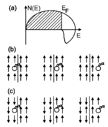
Figure 29: The tunneling transport between strongly correlated ferromagnets. The density of states in the lower Hubbard band (a) is provided by standard current states for majority-spin electrons (above) and by non-quasiparticle states for minority-spin electrons (below), the latter contribution being non-zero only above the Fermi energy (occupied states are shadowed). However, the tunneling is possible both for parallel (b) and antiparallel (c) magnetization directions. Chioncel et al. (2005)

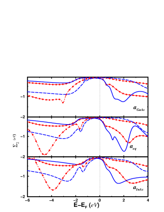
Figure 31: (Color online) Energy dependences of imaginary parts of the electron self-energy $\Sigma_{2}(E)$, for lattice constants of GaAs (a), equilibrium one (b), and of InAs (c): $e_{g}$ down solid line, $t_{2g}$ down decorated solid line, $e_{g}$ up dashed line, $t_{2g}$ up decorated dashed line. Chioncel et al. (2005)

V.2.2 VAs: correlation-induced half-metallic ferromagnetism?

Interesting materials for spintronics applications are ferromagnetic semiconductors Nagaev (1983); Ohno (1998a, b). Candidate systems are ordered compounds such as europium chalcogenides (e.g., EuO) and chromium spinels (e.g., CdCr₂Se₄) Nagaev (1983), as well as diluted magnetic semiconductors (e.g., Ga_1-xMn_xAs) Ohno (1998a, b). Unfortunately, all of them have Curie temperatures much lower than room temperature. On the other hand, VAs in the zinc-blende structure is, according to density-functional calculations Galanakis and Mavropoulos (2003), a ferromagnetic semiconductor with a high Curie temperature. Unlike CrAs Akinaga et al. (2000), CrSb Zhao et al. (2001), and MnAs Okabayashi et al. (2004), VAs has not yet been experimentally fabricated in the zinc-blende structure, but the increasing experimental activity in the field of the (structurally metastable) zinc-blende ferromagnetic compounds is promising in this respect.

The main result including many-body correlation effects is displayed in Fig. 33. While this material is expected to be a ferromagnetic semiconductor from density-functional theory (LSDA/GGA) or static LSDA+$U$ calculations, the inclusion of dynamic Coulomb correlations within the LSDA+DMFT approach predicts a majority-spin band metallic behavior due to the closure of the gap ($\approx$50 meV). However, since the minority-spin band gap ($\simeq 1$eV) remains finite, the material is found to be a half-metallic ferromagnet. To our knowledge, this is a first example where dynamic correlations transform a semiconductor into a half-metal Chioncel et al. (2006b). This remarkable result demonstrates the relevance of many-body effects for spintronic materials.

Figure 32: Schematic representation of the $p$-$d$ hybridization and bonding-antibonding splitting in VAs.Chioncel et al. (2006b)

The important features of the electronic structure of VAs Galanakis and Mavropoulos (2003) are shown schematically in Fig. 32. The $t_{2g}$ states hybridize with the neighboring As $p$ states, forming wide bonding and antibonding hybrid bands. In contrast, the $e_{g}$ states form mainly non-bonding narrow bands. The Fermi level lies between $e_{g}$ and antibonding $t_{2g}$ states in the majority-spin bands, and between bonding $t_{2g}$ and $e_{g}$ in the minority-spin bands. The spin moment, concentrated mainly at the V atoms, is an integer of exactly $M=2$ $\mu_{B}$ per unit formula, which is obvious from counting the occupied bands for two spin directions.

The exchange constants of VAs were calculated within GGA and adiabatic spin dynamics approach, similar to the one used by Halilov et al. Halilov et al. (1998). Using these exchange parameters in a Monte Carlo simulation of the corresponding classical Heisenberg Hamiltonian yields a Curie temperature $T_{C}=820$ K Chioncel et al. (2006b) by the fourth-order cumulant crossing point. This result agrees with the value of $T_{C}=830$ K calculated in Ref.  Sanyal et al. (2003) by using a similar method. The high Curie point is well above the room temperature, which makes VAs a very promising candidate for applications in spintronics.

Static correlations were taken into account within the LDA+$U$ method using similar values of effective interactions parameters $U=2$ eV and $J=0.9$ eV as in the case of Heusler alloys. It will give just an estimation of correlations effects in VAs, since for exact value of $U$ one need to perform a complicated analyse of screening effects in this compound Kotliar et al. (2006); Aryasetiawan et al. (2004). The theoretically determined equilibrium lattice parameter, $a=5.69$Å, and a broadening $\delta$ of about $15$K, which allows the majority spin gap to be clearly resolved, were used. For different lattice parameters (e.g., as for InAs) the LDA results agree with the previous ones Sanyal et al. (2003); Galanakis and Mavropoulos (2003). The GGA DOS is shown in Fig. 33. The main difference in the GGA+$U$ spectrum is that the occupied localized majority $e_{g}$ states are expected to shift to even lower energy, while the unoccupied minority $e_{g}$ states to higher energy. The semiconducting character does not change, since the $e_{g}$ and $t_{2g}$ bands remain separated for both spins; the majority-spin gap slightly increases, but remains small.

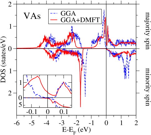
Figure 33: (color online) DOS of VAs within the GGA (dashed blue line) and GGA+DMFT (solid red line) for a temperature of $T$=200 K, $U$=2 eV and $J$=0.9 eV. Inset: Focus around $E_{F}$ showing the semiconducting gap within the GGA. To illustrate the minority-spin NQP states a ten times larger scale for the spin down channel is used.Chioncel et al. (2006b)

In order to investigate dynamic correlation effects in VAs the fully self-consistent in spin, charge and self-energy LSDA+DMFT scheme Chioncel et al. (2003b, a); Chioncel et al. (2005) was used. The computational results for the DFT in the GGA approximation and LDA+DMFT densities of states are presented in Fig. 33. The non-quasiparticle states in the minority spin band are visible just above the Fermi level (inset), predicted also by previous calculations Chioncel et al. (2003a); Chioncel et al. (2005). The weak spectral weight of NQP states is due to that the Fermi level is close to the right edge of the minority spin gap, as discussed for CrAs having a similar structure Chioncel et al. (2005). The local spin moments at V atoms do not change significantly (by less than 5%). However, in the case of VAs another correlation effect appears: the small majority-spin gap at $E_{F}$ closes, making the material half-metallic Chioncel et al. (2006b).

In order to investigate the mechanism of the gap closing for the majority spin channel, the behavior of the electron self-energy was investigated Chioncel et al. (2006b). For the majority-spin, $\mathrm{Im}\Sigma_{\uparrow}(E)\sim(E-E_{F})^{2}$ which indicates a Fermi-liquid behavior, as opposed to $\mathrm{Im}\Sigma_{\downarrow}(E)$ which shows a suppression around $E_{F}$ due to the band gap, as well as a peculiar behavior for $E>E_{F}$ related to the existence of NQP states.

From the Dyson equation (165) one can see that the real part $\mathrm{Re}\Sigma_{\sigma}(E)$ causes a shift of the LDA energy levels. Therefore, due to the non-zero $\Sigma_{\uparrow}^{e_{g}}$, the $e_{g}$ orbitals in the close vicinity of the Fermi level are pushed closer to $E_{F}$. This renormalization is connected with the large absolute value of $\mathrm{Re}(\partial\Sigma/\partial E)_{E_{F}}<0$. This causes occupied levels to be shifted to higher energy and unoccupied levels to lower energy. Note that this effect is completely opposite to the LDA$+U$ results discussed above. In addition to this shift, the $e_{g}$ peak is broadened by correlations, its tail reaching over the Fermi level (Fig. 33, inset). Thus the finite-temperature LDA+DMFT calculations demonstrate the closure of the narrow gap in the spin-up channel, which is produced by the correlation-induced Fermi-liquid renormalization and spectral broadening. At the same time, NQP states appear for the minority-spin channel just above $E_{F}$.

The slope of the majority-spin self-energy is almost a constant as a function of temperature at low $T$: $\mathrm{Re}(\partial\Sigma_{\uparrow}/\partial E)_{E_{F}}\simeq-0.4$ between 200 K and 500 K. The quasiparticle weight, which measures the overlap of the quasiparticle wave function with the original one-electron one for the same quantum numbers, is $Z=(1-\partial\mathrm{Re}\Sigma_{\uparrow}/\partial E)^{-1}\simeq 0.7.$ As a consequence, the closure of the gap in the majority channel is a quantum effect originating from the multi-orbital nature of the local Coulomb interaction (energy states are shifted towards $E_{F}$) rather than an effect of temperature. A similar gap closure is obtained for larger values of $U$, namely, $U=4$ and 6 eV, although the latter values should be taken with some caution in the FLEX calculation, which is in principle appropriate only in weak to intermediate coupling. As a general tendency, increasing $U^{\ast}=U-J$ produces a stronger Fermi-liquid renormalization in the majority spin channel, the same effect being evidenced for $J=0$.

On the one hand, density-functional theory calculations within the GGA (Ref. Chioncel et al. (2006b)) predict this material to be a ferromagnetic semiconductor with a tiny gap of about 50 meV in the majority-spin states and large gap of the order of 1 eV for minority-spin states. Quantum effects, such as spin and orbital fluctuations, described by LDA+DMFT destroy the narrow gap and turn the material into an half-metallic ferromagnet.

On the other hand, several other mechanisms could contribute to the band-gap narrowing with increasing temperature. A well studied example is electron-phonon interaction. In another semiconductor with the zinc-blende structure, GaAs, it amounts to 50meV at 200K Paessler (1999). Also spin-orbit coupling can be essential when considering closing of the gap.

The LDA/GGA calculation supplemented by a Monte Carlo simulation also predicts a high Curie temperature of 830 K Sanyal et al. (2003), which makes this material of interest for technological applications. One can expect that $T_{C}$ is not strongly affected by dynamical correlation, for the same reason as the effective exchange interaction parameters (see recent works Katsnelson and Lichtenstein (2002)).

The revealed half-metallic (instead of semiconducting) behavior has important consequences in the potential applications of VAs in spintronics. In contrast to all semiconductor-based spin-injection devices Zutic et al. (2004) which avoid the resistivity mismatch problem, half-metals can be applied to obtain giant magnetoresistance or, provided that interface states are eliminated Mavropoulos et al. (2005), tunneling magnetoresistance effects. We see that correlation effects play a decisive role in the prediction of new spintronic materials. The metallic nature of the majority spin channel would be visible in resistivity measurements. Therefore, the experimental realization of zinc-blende VAs would provide a test of this prediction. Further research should address the issue of the stability of the half-metallic ferromagnetic state in a zinc-blende structure. Some work in this direction has been already carried out Shirai (2003); Xie et al. (2003b).

V.3 Half-metallic transition metal oxides

V.3.1 CrO₂: a rutile structure half-metallic ferromagnet

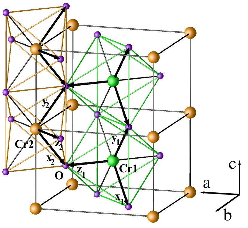
Figure 34: (Color online) CrO₂ (rutile) structure. Cr1 (green) and Cr2 (orange) are located at (0, 0, 0) and $(\frac{1}{2},\frac{1}{2},\frac{1}{2})$. Cr atoms are octahedrally coordinated by oxygen atoms (purple). The local coordinate system is used for each Cr atom; $\hat{\mathbf{x}}_{1}=-\frac{1}{2}\hat{\mathbf{a}}+\frac{1}{2}\hat{\mathbf{b}}-\frac{1}{\sqrt{2}}\hat{\mathbf{c}}$, $\hat{\mathbf{y}}_{1}=-\frac{1}{2}\hat{\mathbf{a}}+\frac{1}{2}\hat{\mathbf{b}}+\frac{1}{\sqrt{2}}\hat{\mathbf{c}}$, $\hat{\mathbf{z}}_{1}=\frac{1}{\sqrt{2}}\hat{\mathbf{a}}+\frac{1}{\sqrt{2}}\hat{\mathbf{b}}$, and $\hat{\mathbf{x}}_{2}=-\frac{1}{2}\hat{\mathbf{a}}-\frac{1}{2}\hat{\mathbf{b}}-\frac{1}{\sqrt{2}}\hat{\mathbf{c}}$, $\hat{\mathbf{y}}_{2}=-\frac{1}{2}\hat{\mathbf{a}}-\frac{1}{2}\hat{\mathbf{b}}+\frac{1}{\sqrt{2}}\hat{\mathbf{c}}$, $\hat{\mathbf{z}}_{2}=-\frac{1}{\sqrt{2}}\hat{\mathbf{a}}+\frac{1}{\sqrt{2}}\hat{\mathbf{b}}$. $\hat{\mathbf{x}}_{1,2}$ and $\hat{\mathbf{y}}_{1,2}$ are approximately point to $O$ atom, and $\hat{\mathbf{z}}_{1,2}$ are exactly point to $O$ atom. The local axes are transformed into each other by a 90^∘ rotation around the crystal $c$ axis. Yamasaki et al. (2006)

Chromium dioxide CrO₂ has a rutile structure with $a=4.421$ Å, $c=2.916$ Å ($c/a=0.65958$) and internal parameter $u=0.3053$. Porta et al. (1972) The Cr atoms form a body-center tetragonal lattice and are surrounded by a slightly distorted octahedron of oxygen atoms. The space group of this compound is non-symmorphic ($P4_{2}/mnm=D_{4h}^{14}$). The Cr ions are in the center of CrO₆ octahedra, so that the $3d$ orbitals are split into a $t_{2g}$ triplet and an excited $e_{g}$ doublet. The $e_{g}$ states with only two valence $3d$ electrons are irrelevant, and only the $t_{2g}$ orbitals are to be considered. The tetragonal symmetry distorts the octahedra, which lifts the degeneracy of the $t_{2g}$ orbitals into a $d_{xy}$ ground state and $d_{yz+zx}$ and $d_{yz-zx}$ excited states Lewis et al. (1997); Korotin et al. (1998) (see Fig. 34, a local coordinate system is used for every octahedron). A double exchange mechanism for two electrons per Cr site was proposed Schlottmann (2003). According to this, the strong Hund’s rule together with the distortion of CrO₆ octahedra leads to localization of one electron in the $d_{xy}$ orbital, while the electrons in the $d_{yz}$ and $d_{xz}$ are itinerant.

Measurements of the magnetic susceptibility in the paramagnetic phase show a Curie-Weiss-like behavior indicating the presence of local moments Chamberland (1977), which suggests a mechanism of ferromagnetism beyond the standard band or Stoner-like model.

Several recent experimental investigations of photoemission Tsujioka et al. (1997), soft x-ray absorption Stagarescu et al. (2000), resistivity  Suzuki and Tedrow (1998), and optics Singley et al. (1999) suggest that electron correlations are essential for the underlying physical picture in CrO₂. Schwarz Schwarz (1986) first predicted the half-metallic band structure with a spin moment of $2\mu_{B}$ per formula unit for CrO₂. Lewis Lewis et al. (1997) used the plane-wave potential method and investigated the energy bands and the transport properties, characterizing CrO₂ as a “bad metal” (a terminology applied earlier to high temperature superconductors and to other transition metal oxides, even ferromagnets like SrRuO₃). A decade later the LSDA+$U$ calculation Korotin et al. (1998) treated the conductivity in the presence of large on-site Coulomb interactions and described CrO₂ as a negative charge-transfer gap material with a self-doping. Contrary to the on-site strong correlation description, transport and optical properties obtained within the FLAPW method (LSDA and GGA) Mazin et al. (1999) suggest that the electron-magnon scattering is responsible for the renormalization of the one-electron bands. More recent model calculations Laad et al. (2001); Craco et al. (2003) propose even orbital correlations.

Figure 35: Full basis set spin-polarized (ferromagnetic) bands for CrO₂; majority spin (left) and minority spin (right). $E_{F}$ is set to be zero. The high-symmetry points are $\Gamma(0,0,0)$, $X(0,\frac{1}{2},0)$, $M(\frac{1}{2},\frac{1}{2},0)$, $Z(0,0,\frac{1}{2})$, $R(0,\frac{1}{2},\frac{1}{2})$, $A(\frac{1}{2},\frac{1}{2},\frac{1}{2})$. Yamasaki et al. (2006)

Chemical bonding in rutile-type compounds including CrO₂ was analyzed by Sorantin and Schwarz Sorantin and Schwarz (1992). One can see that around the Fermi level the bands are primarily chromium $3d$ states of $t_{2g}$ manifold, with $e_{g}$ bands being situated higher in energy due to the crystal-field splitting. In the spin polarized case, the exchange splitting shifts the minority spin $d$ bands above the Fermi level (Fig. 35). For the majority $t_{2g}$ bands the Fermi level lies in a pseudogap. Oxygen $p$ $-$ chromium $d$ hybridization creates both bonding and antibonding hybrid orbitals, with the bonding orbital appearing in the occupied part and the antibonding hybrid orbital remaining in the Cr $t_{2g}$ manifold. Half of the $d_{yz}$ and $d_{zx}$ components of $t_{2g}$ are pushed upward by antibonding, which explains the $d_{xy}$ dominance in the spin density. The non-magnetic DOS shows a sharp peak at the Fermi level, which signals the magnetic instability according to the usual Stoner argument.

Although there is a significant difference between the $t_{2g}$ and $e_{g}$ orbitals  Schwarz (1986); Sorantin and Schwarz (1992); Korotin et al. (1998); Mazin et al. (1999), the analysis in the framework of NMTO technique Andersen and Saha-Dasgupta (2000); Zurek et al. (2005) shows that their interplay is important not only for the crystal-field splitting of $t_{2g}$ states, but also for the general bonding in the rutile structure. The $t_{2g}$ orbitals form the basis set used in Ref. Yamasaki et al. (2006) to evaluate the effective hopping Hamiltonian matrix elements.

In CrO₂ the bands around the Fermi level are primarily chromium $3d$ states of $t_{2g}$ manifold, $e_{g}$ bands being situated higher in energy owing to crystal-field splitting. The $t_{2g}$ orbitals are further split into single $d_{xy}$ and nearly degenerate $d_{yz\pm zx}$ bands owing to the orthorhombical distortion of CrO₆ octahedra. Despite the differences between Cr $t_{2g}-e_{g}$ orbitals, their interaction plays an important role not only in characterizing the crystal-field splitting, but also in the general picture of bonding in the rutile structure.

Concerning the Coulomb interaction $U$ in CrO₂, the higher energy $e_{g}$ bands, although making no noticeable contribution at the Fermi level, could participate in the screening of the $t_{2g}$ orbitals Solovyev et al. (1996); Pickett et al. (1998), thereby giving the values $U=3~{}$eV and $J=0.87$ eV.

Previous LSDA$+U$ Korotin et al. (1998); Toropova et al. (2005) and DMFT Laad et al. (2001); Craco et al. (2003) studies yielded independently a narrow almost flat band of $d_{xy}$ character, which produces ferromagnetism in CrO₂. In contrast to these results, the fully self-consistent LSDA+DMFT Chioncel et al. (2007) yields, in agreement with a non-local variational cluster approach Chioncel et al. (2007), an itinerant $d_{xy}$ orbital which crosses the Fermi level. Despite the non-localized character of the orbital, a ferromagnetic phase is still obtained.

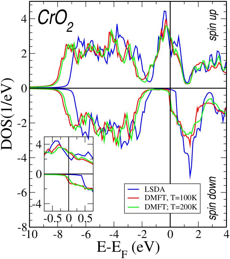
Figure 36: (Color online) Density of states obtained within the LSDA and LSDA+DMFT calculations for different temperatures. The inset shows the results for a smaller energy window around the Fermi level. Chioncel et al. (2007)

Results of the LSDA+DMFT calculation are presented in Fig. 36 for two different values of $T$ and compared with the LSDA results. The LSDA Fermi level intersects the majority-spin bands near a local minimum and lies in the band gap of the minority spin. Finite temperatures and correlation effects close this pseudogap around the Fermi level, as can be seen from the LDA+DMFT results in Fig.36. No differences can be observed between the two DMFT results at different temperatures, except for the smearing of DOS features at larger temperature. For both spin channels the DOS is shifted uniformly to lower energies in the energy range $-2\div-6$ eV, where predominantly the O($p$) bands are situated. This is due to the Cr($d$) bands which affect the O($p$) states through the Cr($d$)$-$O($p$) hybridization, so that O($p$) states contribute actively to the ferromagnetic ground state formation.

Fig. 37 presents the experimentally measured spin polarization Huang et al. (2003) in comparison with the theoretical calculations within the LSDA and finite temperature LDA+DMFT (T=200 K) Chioncel (2006). Resonant X-ray emission spectroscopy Kurmaev et al. (2003) showed the existence of nearly currentless minority spin states in the vicinity of the Fermi level, which can be connected to the non-quasiparticle states III.10. As described in previous sections IV.1 and V electronic structure of several half-metallic ferromagnets reveal the existence of such NQP states, which are important for the proper description of spin polarization near the Fermi level. The LSDA+DMFT description, however, is not sufficient to capture the high energy tail of the experimental spin polarization. This can be related with improper description of unoccupied Cr $e_{g}$ orbitals in the LSDA, and probably, also with non-local exchange effects which can be investigated within a cluster DMFT scheme Kotliar et al. (2006).

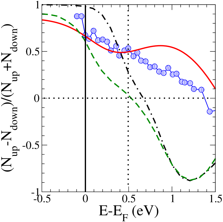
Figure 37: (Color online) Energy dependence of spin-polarization of CrO₂. Experimental measurement blue scattered line Huang et al. (2003), LSDA calculation (black dot-dashed), DMFT (green dashed) and non-local variational approach, red continuous line Chioncel et al. (2007).

The NQP states occur around 0.25 eV in the spin-down channel. At zero temperatures, the variational cluster results Chioncel et al. (2007) yield the states in the minority channel which are actually far from $E_{F}$, but have a tail vanishing at $E_{F}$. This is in agreement with low temperature experiments Soulen et al. (1998); Ji et al. (2001) which support very high polarization of CrO₂.

The effects of local and non-local electronic correlations in CrO₂ Chioncel et al. (2007) change considerably the mean-field LSDA$+U$ picture, despite the interaction is not too strong. In particular, in LSDA$+U$ the single occupancy of the Cr $d_{xy}$ orbital is determined by the exchange and crystal-field splitting. On the other hand, the competition of the latter with correlation effects, which is taken into account in the DMFT and variational cluster perturbation theory calculations, induces a ferromagnetic state with itinerant-type $d_{xy}$ orbitals possessing a large effective mass rather than with localized moments, in contrast to previous results Korotin et al. (1998); Toropova et al. (2005); Laad et al. (2001); Craco et al. (2003). In the minority-spin channel, correlations induce NQP states which are crucial for the occurrence of spin depolarization in CrO₂. However, a quantitative analysis of the depolarization would require the inclusion of additional effects, e.g., disorder or phonons (sect. III.3).

VI Exchange interactions and critical temperatures in half-metallic compounds

Owing to the strong interest in the half-metallic ferromagnetism, the number of theoretical studies of exchange interactions and calculations of Curie temperatures in Heusler alloys has been drastically increased last time (see, e.g., recent review Zhang et al. (2007)). The first investigations of the exchange interactions in half-metals within the DFT formalism was made by Kübler Kübler et al. (1983). The mechanisms of ferromagnetism in Heusler alloys were discussed on the basis of total-energy calculations for the ferro- and antiferromagnetic configurations. Since the antiferromagnetic state of the system is not half-metallic, such an estimation gives only crude values of exchange parameters in HMF. Therefore, a more precise evaluation of the exchange interactions from the first-principle theory is required. In this section we present the real-space Green’s function and frozen-magnon techniques to calculate the exchange parameters, and their applications to full-Heusler, semi-Heusler, and zinc-blende half-metals.

VI.1 The Green’s function formalism

Within the first-principle Green’s function approach the exchange parameters are obtained by mapping the second variation of electronic band energy to the classical Heisenberg Hamiltonian and making use of magnetic version of the Andersen’s local force theorem Machintosh and Andersen (1980).

$$H_{eff}=-\frac{1}{2}\sum_{\mu,\nu}\sum_{RR^{\prime}}J_{\bf RR^{\prime}}^{\mu,\nu}{\bf s}_{\bf R}^{\mu}{\bf s}_{\bf R^{\prime}}^{\nu}$$ (200)

In Eq. (200), the indices $\mu$ and $\nu$ mark different sublattices, ${\bf R}$ and ${\bf R^{\prime}}$ are the lattice vectors specifying the atoms within a sublattice, ${\bf s}_{\bf R}^{\mu}$ is the unit vector in the direction of the magnetic moment. By introducing the generalized notation for site $(i=\mu,{\bf R})$, a simple and transparent expression for the exchange interaction parameters is obtained in the following form Liechtenstein et al. (1987):

$$J_{ij}=\frac{1}{4\pi}\int d\epsilon ImTr_{L}\{\Delta_{i}G_{ij}^{\uparrow}\Delta_{j}G_{ij}^{\downarrow}\},$$ (201)

where $G_{ij}^{\sigma}$ is the real space Green’s function and $\Delta_{i}$ is the local exchange splitting for site $i$.

VI.2 The frozen-magnon approach and DFT calculations of spin spirals

The approach is based on the evaluation of the energy of the frozen-magnon configurations defined by the following atomic polar and azimuthal angles:

$$\theta_{\bf R}^{\mu}=\theta;\\ {\phi}_{\bf R}^{\mu}={\bf q\cdot R}+{\phi}^{\mu}$$ (202)

The angle $\theta$ defines the cone of the spin spiral, and the constant phase ${\phi}^{\mu}$ is normally chosen to be zero. The magnetic moments of other sublattices are kept parallel to the z-axis. Within the classical Heisenberg model (200) the energy of the spin-spiral configuration is

$$E^{\mu\mu}(\theta,{\bf q})=E^{\mu\mu}_{0}(\theta)+J^{\mu\mu}({\bf q})\cdot sin^{2}\theta$$ (203)

where $E^{\mu\mu}_{0}(\theta)$ does not depend on $q$ and the Fourier transform $J^{\mu\mu}({\bf q})$ is defined by:

$$J^{\mu\nu}({\bf q})=\sum_{\bf R}J^{\mu\nu}_{0\bf R}exp(i{\bf q\cdot R})$$ (204)

In the case where $\nu=\mu$ the sum in Eq. (204) does not include the local interaction with $R=0$. Calculating $E^{\mu\mu}(\theta,{\bf q})$ for a regular $q$-mesh in the Brillouin zone of the crystal and performing the inverse Fourier transformation one gets exchange parameters $J^{\mu\mu}_{0\bf R}$ for sublattice $\mu$.

The Curie temperature can be estimated within the mean-field (MFA),

$$k_{B}T_{C}^{MFA}=\frac{2}{3}\sum_{\bf R}J^{\mu\nu}_{0\bf R}=\frac{M}{6\mu_{B}}\frac{1}{N}\sum_{\bf q}\omega({\bf q})$$ (205)

and random phase approximation (RPA)

$$\frac{1}{k_{B}T_{C}^{RPA}}==\frac{6\mu_{B}}{M}\frac{1}{N}\sum_{\bf q}\frac{1}{\omega({\bf q})}$$ (206)

with $\omega(q)$ the spin-wave dispersion, $N$ the number of $q$ points in the first Brillouin zone, and $M$ the atomic magnetic moment. In the MFA the Curie temperature is determined by the arithmetic average of the magnon energies, while in the RPA $T_{C}$ is determined by the harmonic average. Therefore the value of $T_{C}$ within MFA is larger than the RPA one, the two values being equal only provided that the magnon spectrum is dispersionless.

VI.3 First-principle calculations

VI.3.1 Semi-Heusler C1_b alloys

First-principle studies of exchange interactions and magnetic phase transitions for NiCrZ (Z=P,Se,Te), NiVAs, NiMnSb, CoMnSb were carried out by many authors Sasioglu et al. (2005b); Rusz et al. (2006) In fig. 38 the frozen-magnon dispersion and the exchange interactions are presented Sasioglu et al. (2005b). The exchange interactions are Fourier transforms of the frozen-magnon spectrum.

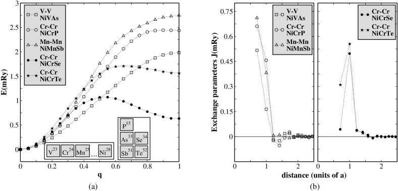
Figure 38: Left pannel(a): Frozen-magnon dispersion for NiCrZ (Z=P,Se,Te). Right pannel(b): Interatomic exchange interactions. Sasioglu et al. (2005b).

A remarkable feature of the exchange interactions is their short-range character, the Curie temperature being determined by the interaction within first two coordination spheres. The deviation from the collinear alignment of magnetic moments can be also characterized by magnon energies Sandratskii (1998); Sandratskii and Bruno (2003). The deviation leads to the mixing of the majority and minority spin states, which makes half-metallicity less favorable. A detailed discussion of different depolarization mechanisms is given in section III.3.

VI.3.2 Full-Heusler L2₁ alloys

Recently the studies of the interatomic exchange interactions in several full-Heusler compounds were reported by Kurtulus et al. Kurtulus et al. (2005) Sasioglu et al. studied the exchange interactions in non-half-metallic Ni₂MnZ (Z=Ga, In, Sn, Sb) and half-metallic Mn₂VZ (Z=Al,Ge). The importance of the intersublattice exchange interactions has been demonstrated. For Mn₂VZ (Z=Al,Ge) it was shown that the ferrimagnetic coupling between the V and Mn moments stabilizes the ferromagnetic alignment of the Mn moments.

In Co₂MnZ (Z=Ga, Si, Ge, Sn) the presence of Co atoms makes the interaction more complicated Kurtulus et al. (2005). The interaction between the Co atoms in the same sublattice ,Co1(2)-Co1(2), and between Co atoms at different sublattices, Co1(2)-Co2(1) has to be taken into account. This approach gives results which goes beyond the initial approach of Kübler Kübler et al. (1983). From the $J_{ij}$ values it is clear that the exchange interactions are relatively short ranged and do not exceed the first four neighbors in each sublattice. The main exchange parameter corresponds to the nearest neighbor Co(1)-Mn interaction. This already gives 70$\%$ of the total contribution to $J$ and is about ten times larger than the Co-Co and Mn-Mn interactions Kurtulus et al. (2005). Thus, it was concluded that the Co-Mn interactions are responsible for the stability of ferromagnetism (see Fig. 39).

The interaction changes weakly with the contraction of the lattice Sasioglu et al. (2005c) interactions between Co at different sublattices favors ferromagnetism and is stronger than the ferromagnetic interaction between the Mn atoms. The intrasublattice Mn-Mn ad Co-Co interactions have different signs for different distances between atoms, which means a RKKY-type interaction.

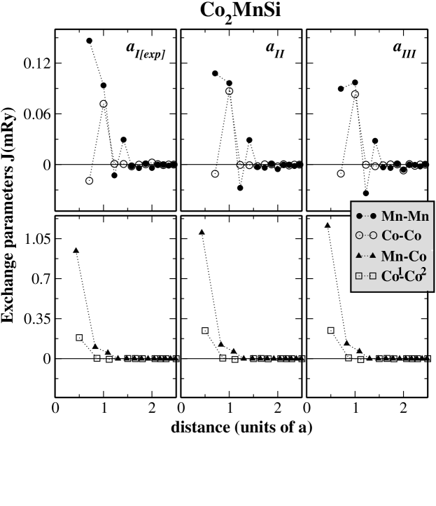
Figure 39: Exchange constants for Co₂MnSi as a function of interatomic distance. Sasioglu et al. (2005c).

VI.3.3 Zinc-blende half-metals

Besides the large number of results on the electronic properties of zinc-blende half-metals, the exchange interactions constitute an important aspect to understand the stability of half-metallicity in these structures. Shirai Shirai (2003) obtained that in VAs, CrAs and MnAs ferromagnetism is energetically favorable in comparison with the antiferromagnetic state, unlike FeAs where an opposite effect was demonstrated. Sakuma Sakuma (2002) predicted ferromagnetism in the isoelectronic MnSi, MnGe and MnSn compounds. Similarly to CrAs, the ferromagnetism in these systems is stabilized by short-range interactions (direct Mn-Mn and indirect through sp atoms), giving a Curie temperature of 1000K Sakuma (2002). $T_{C}$ for the VAs, CrAs and MnAs was calculated also by Kübler Kübler (2003) yielding the same range of magnitudes. Using GaAs and InAs lattice constants, Sanyal et al Sanyal et al. (2003) calculated $T_{C}$ for VAs, CrAs and MnAs. Sasioglu et al Sasioglu et al. (2005a) calculated the exchange parameters for a large number of pnictides.

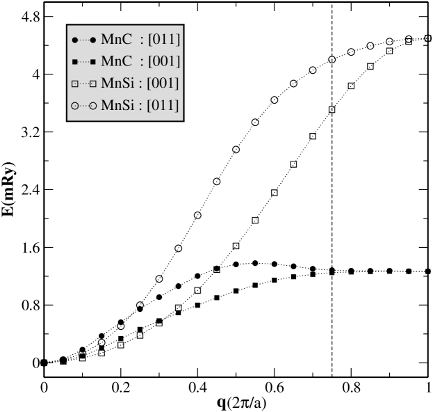
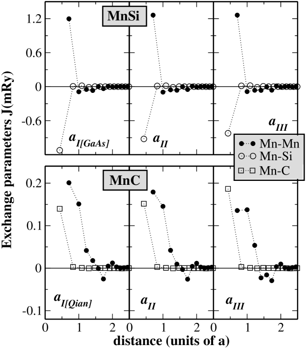
Figure 40: Upper pannel: Frozen-magnon energies for MnC and MnSi in the $[00q]$ and $[0qq]$ directions. Vertical broken line shows the Brillouin zone boundary. Lower panel: Exchange constants as a function of interatomic distance. Sasioglu et al. (2005a).

MnC presents an interesting situation since its half-metallic gap is situated in majority spin channel. The Curie temperature was found to be 500K. Fig.40 represents the frozen-magnon energies for a selected direction in the Brillouin zone and the exchange constants. Ferromagnetism is stabilized by the direct Mn–Mn interactions and Mn-C ferromagnetic coupling. A remarkable feature of MnC is small difference between the MFA and RPA values of $T_{C}$.Sasioglu et al. (2005a).

VII Conclusions

The idea of half-metallic ferromagnetism appeared as a result of band-structure calculations de Groot et al. (1983b). During a long time, dominant activity in this field was theoretical. Conceptually, HMF are of interest from the point of view they provide an opportunity to probe in a clear form some essentially many-particle effects Irkhin and Katsnelson (1990). Whereas for generic metallic system the Landau Fermi-liquid theory Nozieres (1964); Vonsovsky and Katsnelson (1989) works, most correlation effects being hidden in a parameter renormalization (such as effective mass, magnetic moment etc.), in HMF the spin-polaronic effects lead to a qualitatively new feature: occurrence of non-quasiparticle (incoherent) states in the energy gap for one of spin projections near the Fermi level. On the contrary, similar effects of electron-magnon interactions in traditional itinerant-electron ferromagnets are mixed with other kind renormalizations (e.g., electron-phonon, electron-electron ones etc.). The NQP states occur only above (below) $E_{F}$ for minority spin (majority spin) gap. Therefore HMF are ideal objects to investigate effects of electron-magnon interactions Irkhin and Katsnelson (1990).

Even stronger motivation to study HMF is connected with perspectives to use them in giant magnetoresistance and tunnel magnetoresistance de Groot et al. (1983a); Irkhin and Katsnelson (1994); Prinz (1998) devices. This initiated great theoretical activity in the field of heterostructures containing HMF Tkachov et al. (2001); Irkhin and Katsnelson (2002). At the same time, the interest in the search and prediction of new HMF was growing on the basis of band-structure calculations, as well as attempts to understand better the features of electronic structure and chemical bonding which are relevant for half-metallicity (see Sect.V).

Recently, numerous attempts have been performed to build heterostructures with HMF, such as Heusler alloys Sakuraba et al. (2006b, a); Sakuraba et al. (2007); Gercsi et al. (2006), CrO₂ Miao et al. (2006), Fe₃O₄ Zhao et al. (2006); Rybchenko et al. (2006). Therefore the half-metallicity predicted by electronic structure calculations becomes practically applicable. Nevertheless, direct experimental evidences of half-metallic structure for specific compounds are still rather poor. Perhaps, the unique method of testing genuine, bulk, half-metallic properties remains the spin-resolved positron annihilation. This underexposed technique enables the direct measurement of the spin-polarization in the bulk. Advanced techniques borrowed from semiconductor technologies which access spatially resolved spin polarization at the Fermi level would be interesting alternatives for positron annihilation. Although being extensively used to characterize semiconductors, they are poorly known for the spintronics community.

Among other experiments expected to advance the field we mention the STM Irkhin and Katsnelson (2006), spin-polarized photoemission Park et al. (1998), and Andreev reflection Soulen et al. (1999). Investigations of nuclear magnetic relaxation rate should be specially mentioned since the absence of the Korringa relaxation is a clear sign of the half-metallicity Irkhin and Katsnelson (2001) and NMR gives is not surface sensitive and gives direct information on bulk properties. Also data of core-level spectroscopies, especially XMCD would be very useful (see Sect.III.10). As for the band-structure calculations, application of state-of-art methods taking into account correlation effects, such as GW or DMFT (see Sect.IV.1) looks very promising. Another perspective direction is the use of electron-structure calculations to search essentially new types of HMF like $sp$ electron (or anionic) magnets Edwards and Katsnelson (2006); Attema et al. (2005).

References

- Abragam (1961) Abragam, A., 1961, The Principles of Nuclear Magnetism (Clarendon, Oxford).
- Akinaga et al. (2000) Akinaga, H., T. Magano, and M. Shirai, 2000, Jpn. J. Appl. Phys. 39(11B), L1118.
- Almbladh et al. (1999) Almbladh, C.-O., U. V. Barth, and R. V. Leeuwen, 1999, Int. J. Mod. Phys. B 13(5-6), 535.
- Andersen (1975) Andersen, O. K., 1975, Phys. Rev. B 12(8), 3060.
- Andersen and Jepsen (1984) Andersen, O. K., and O. Jepsen, 1984, Phys. Rev. Lett. 53(27), 2571.
- Andersen and Saha-Dasgupta (2000) Andersen, O. K., and T. Saha-Dasgupta, 2000, Phys. Rev. B 62(24), R16219.
- Anisimov et al. (1997a) Anisimov, V. I., F. Aryasetiawan, and A. I. Lichtenstein, 1997a, J. Phys.: Condens. Matter 9, 767.
- Anisimov and Gunnarsson (1991) Anisimov, V. I., and O. Gunnarsson, 1991, Phys. Rev. B 43(10), 7570.
- Anisimov et al. (1997b) Anisimov, V. I., A. I. Poteryaev, M. A. Korotin, A. O. Anokhin, and G. Kotliar, 1997b, J. Phys.: Condens. Matter 9(35), 7359.
- Anisimov et al. (1993) Anisimov, V. I., I. V. Solovyev, M. A. Korotin, M. T. Czyżyk, and G. A. Sawatzky, 1993, Phys. Rev. B 48(23), 16929.
- Anokhin and Katsnelson (1996) Anokhin, A. O., and M. I. Katsnelson, 1996, Int. J. Mod. Phys. B 10, 2468.
- Antonov et al. (1999) Antonov, V. N., V. P. Antropov, B. N. Harmon, A. N. Yaresko, and A. Y. Perlov, 1999, Phys. Rev. B 59(22), 14552.
- Antonov et al. (1997) Antonov, V. N., P. M. Oppeneer, A. N. Yaresko, A. Y. Perlov, and T. Kraft, 1997, Phys. Rev. B 56(20), 13012.
- Aryasetiawan et al. (2004) Aryasetiawan, F., M. Imada, A. Georges, G. Kotliar, S. Biermann, and A. I. Lichtenstein, 2004, Phys. Rev. B 70(19), 195104.
- Attema et al. (2004) Attema, J. J., C. M. Fang, L. Chioncel, G. A. de Wijs, A. I. Lichtenstein, and R. A. de Groot, 2004, J. Phys.: Condens. Matter 16, S5517.
- Attema et al. (2005) Attema, J. J., G. de Wijs, G. R. Blake, and R. A. de Groot, 2005, Journal of the American Chemical Society 127(46), 16325.
- Attema et al. (2006) Attema, J. J., G. A. de Wijs, and R. A. de Groot, 2006, J. Phys. D: Appl. Phys. 39, 793.
- Auslender and Irkhin (1984a) Auslender, M. I., and V. Y. Irkhin, 1984a, Z. Phys. B 56, 301.
- Auslender and Irkhin (1984b) Auslender, M. I., and V. Y. Irkhin, 1984b, Solid State Commun. 50, 1003.
- Auslender and Irkhin (1985a) Auslender, M. I., and V. Y. Irkhin, 1985a, Z. Phys. B 61, 129.
- Auslender and Irkhin (1985b) Auslender, M. I., and V. Y. Irkhin, 1985b, Solid State Commun. 56(8), 701.
- Auslender et al. (1988) Auslender, M. I., V. Y. Irkhin, and M. I. Katsnelson, 1988, J. Phys. C 21, 5521.
- Auslender and Katsnelson (1982) Auslender, M. I., and M. I. Katsnelson, 1982, Teor. Mat. Fiz. 51, 436.
- Auslender et al. (1983) Auslender, M. I., M. I. Katsnelson, and V. Y. Irkhin, 1983, Physica B 119, 309.
- Auth et al. (2003) Auth, N., G. Jakob, T. Block, and C. Felser, 2003, Phys. Rev. B 68(2), 024403.
- Baym and Kadanoff (1961) Baym, G., and L. P. Kadanoff, 1961, Phys. Rev. 124(2), 287.
- Bickers and Scalapino (1989) Bickers, N. E., and D. J. Scalapino, 1989, Ann. Phys. 193, 206.
- Biermann et al. (2003) Biermann, S., F. Aryasetiawan, and A. Georges, 2003, Phys. Rev. Lett. 90(8), 086402.
- de Boer and Groot (1999) de Boer, P. K., and R. A. d. Groot, 1999, Phys. Rev. B 60(15), 10758.
- Bona et al. (1985) Bona, G. L., F. Meier, M. Taborelli, E. Bucher, and P. H. Schmidt, 1985, Solid State Commun. 56(4), 391.
- Borca et al. (2001) Borca, C. N., T. Komesu, H.-K. Jeong, P. A. Dowben, D. Ristoiu, C. Hordequin, J. P. Nozières, J. Pierre, S. Stadler, and Y. U. Idzerda, 2001, Phys. Rev. B 64(5), 052409.
- Bowen et al. (2003) Bowen, M., M. Bibes, A. Barthelemy, J.-P. Contour, A. Anane, Y. Lemaitre, and A. Fert, 2003, Appl. Phys. Lett. 82(2), 233.
- Bratkovsky (1997) Bratkovsky, A. M., 1997, Phys. Rev. B 56(5), 2344.
- Bratkovsky (1998) Bratkovsky, A. M., 1998, Appl. Phys. Lett. 72(18), 2334.
- Brown et al. (2000) Brown, P. J., K. U. Neumann, P. J. Webster, and K. R. A. Ziebeck, 2000, J. Phys.: Condens. Matter 12(8), 1827.
- Carneiro and Pethick (1975) Carneiro, G. M., and C. J. Pethick, 1975, Phys. Rev. B 11(3), 1106.
- Ceperley and Alder (1980) Ceperley, D. M., and B. J. Alder, 1980, Phys. Rev. Lett. 45(7), 566.
- Chadov et al. (2006) Chadov, S., J. Minar, H. Ebert, A. Perlov, L. Chioncel, M. I. Katsnelson, and A. I. Lichtenstein, 2006, Phys. Rev. B 74(14), 140411.
- Chamberland (1977) Chamberland, B. L., 1977, CRC Crit. Rev. Solid State Mater. Sci. 7, 1.
- Chiba et al. (2003) Chiba, D., K. Takamura, F. Matsukura, and H. Ohno, 2003, Applied Physics Letters 82(18), 3020.
- Chioncel (2004) Chioncel, L., 2004, Finite Temperature Electronic Structure, beyond Local Density Approximation, (PhD Thesis, Radbout University Nijmegen).
- Chioncel (2006) Chioncel, L., 2006, unpublished .
- Chioncel et al. (2007) Chioncel, L., H. Allmaier, E. Arrigoni, A. Yamasaki, M. Daghofer, M. I. Katsnelson, and A. I. Lichtenstein, 2007, Phys. Rev. B 75(14), 140406.
- Chioncel et al. (2006a) Chioncel, L., E. Arrigoni, M. I. Katsnelson, and A. I. Lichtenstein, 2006a, Phys. Rev. Lett. 96(13), 137203.
- Chioncel et al. (2003a) Chioncel, L., M. I. Katsnelson, R. A. de Groot, and A. I. Lichtenstein, 2003a, Phys. Rev. B 68(14), 144425.
- Chioncel et al. (2005) Chioncel, L., M. I. Katsnelson, G. A. de Wijs, R. A. de Groot, and A. I. Lichtenstein, 2005, Phys. Rev. B 71(8), 085111.
- Chioncel et al. (2006b) Chioncel, L., P. Mavropoulos, M. Lezaic, S. Blugel, E. Arrigoni, M. I. Katsnelson, and A. I. Lichtenstein, 2006b, Phys. Rev. Lett. 96(19), 197203.
- Chioncel et al. (2003b) Chioncel, L., L. Vitos, I. A. Abrikosov, J. Kollar, M. I. Katsnelson, and A. I. Lichtenstein, 2003b, Phys. Rev. B 67(23), 235106.
- Chitra and Kotliar (2000) Chitra, R., and G. Kotliar, 2000, Phys. Rev. B 62(19), 12715.
- Chitra and Kotliar (2001) Chitra, R., and G. Kotliar, 2001, Phys. Rev. B 63(11), 115110.
- Correa et al. (2006) Correa, J. S., C. Eibl, G. Rangelov, J. Braun, and M. Donath, 2006, Phys. Rev. B 73(12), 125316.
- Craco et al. (2003) Craco, L., M. S. Laad, and E. Müller-Hartmann, 2003, Phys. Rev. Lett. 90(23), 237203.
- Craco et al. (2006) Craco, L., M. S. Laad, and E. Müller-Hartmann, 2006, Phys. Rev. B 74(6), 064425.
- Dagotto (2003) Dagotto, E., 2003, Nanoscale Phase Separation and Colossal Magnetoresistance: The Physics of Manganites and Related Compounds (Springer, Berlin).
- Dederichs et al. (1984) Dederichs, P. H., S. Blügel, R. Zeller, and H. Akai, 1984, Phys. Rev. Lett. 53(26), 2512.
- Delves and Lewis (1963) Delves, R., and B. Lewis, 1963, J. Phys. Chem. Solids 28, 549.
- Dowben and Skomski (2003) Dowben, P. A., and R. Skomski, 2003, J. Appl. Phys. 93(10), 7948.
- Dowben and Skomski (2004) Dowben, P. A., and R. Skomski, 2004, 95(11), 7453.
- Ebert (1996) Ebert, H., 1996, Reports on Progress in Physics 59(12), 1665.
- Ebert and Schutz (1991) Ebert, H., and G. Schutz, 1991, J. Appl. Phys. 69(8), 4627.
- Edwards (1983) Edwards, D. M., 1983, J. Phys. C 16, L327.
- Edwards (2002) Edwards, D. M., 2002, Adv. Phys. 51, 1259.
- Edwards and Hertz (1973) Edwards, D. M., and J. A. Hertz, 1973, Journal of Physics F-Metal Physics 3(12), 2191.
- Edwards and Katsnelson (2006) Edwards, D. M., and M. I. Katsnelson, 2006, J. Phys.: Condens. Matter 18, 7209.
- Eerenstein et al. (2002) Eerenstein, W., T. T. M. Palstra, S. S. Saxena, and T. Hibma, 2002, Phys. Rev. Lett. 88(24), 247204.
- Egorushkin et al. (1983) Egorushkin, V., S. Kulkov, and S. Kulkova, 1983, Physica 123B, 61.
- van Engen et al. (1983) van Engen, P. G., K. H. J. Buschow, R. Jongebreur, and M. Erman, 1983, Appl. Phys. Lett. 42(2), 202.
- Etgens et al. (2004) Etgens, V. H., P. C. de Camargo, M. Eddrief, R. Mattana, J. M. George, and Y. Garreau, 2004, Phys. Rev. Lett. 92(16), 167205.
- Fazekas et al. (1990) Fazekas, P., B. Menge, and E. Müller-Hartmann, 1990, Z. Phys. B 78, 69.
- Fecher et al. (2006) Fecher, G. H., H. C. Kandpal, S. Wurmehl, C. Felser, and G. Schonhense, 2006, J. Appl. Phys. 99(8), 08J106.
- Flatte and Vignale (2001) Flatte, M. E., and G. Vignale, 2001, Appl. Phys. Lett. 78(9), 1273.
- Folkerts et al. (1987) Folkerts, W., G. Sawatzky, C. Haas, R. de Groot, and F. Hillebrecht, 1987, Journal of Physics C - Solid State Physics 20(26), 4135.
- Fong et al. (2004) Fong, C. Y., M. C. Qian, J. E. Pask, L. H. Yang, and S. Dag, 2004, Appl. Phys. Lett. 84(2), 239.
- Fujii et al. (1995) Fujii, S., S. Ishida, and S. Asano, 1995, J. Phys. Soc. Jpn. 64, 184.
- Fukuda et al. (1994) Fukuda, R., T. Kotani, Y. Suzuki, and S. Yokojima, 1994, Prog. Theor. Phys. 92, 833.
- Furukawa (2000) Furukawa, N., 2000, J. Phys. Soc. Jpn. 69, 1954.
- Galanakis (2003) Galanakis, I., 2003, J. Phys.: Condens. Matter 14, 6329.
- Galanakis (2004) Galanakis, I., 2004, J. Phys.: Condens. Matter 16, 3089.
- Galanakis et al. (2002a) Galanakis, I., P. H. Dederichs, and N. Papanikolaou, 2002a, Phys. Rev. B 66(13), 134428.
- Galanakis et al. (2002b) Galanakis, I., P. H. Dederichs, and N. Papanikolaou, 2002b, Phys. Rev. B 66(17), 174429.
- Galanakis and Dederichs (eds.) Galanakis, I., and P. H. Dederichs(eds.), 2005, Lecture Notes in Physics (Springer, Berlin Heidelberg).
- Galanakis and Mavropoulos (2003) Galanakis, I., and P. Mavropoulos, 2003, Phys. Rev. B 67(10), 104417.
- Galanakis and Mavropoulos (2007) Galanakis, I., and P. Mavropoulos, 2007, J. Phys.: Condens. Matter 19, 315213.
- Galanakis et al. (2006) Galanakis, I., P. Mavropoulos, and P. H. Dederichs, 2006, J. Phys. D: Appl. Phys. 39, 765.
- Galitski (1958) Galitski, V. M., 1958, Zh. Eksper. Teor. Fiz. 34, 1011.
- Garsia and Sabias (2004) Garsia, J., and G. Sabias, 2004, J. Phys.: Condens. Matter 16, R145.
- Georges et al. (1996) Georges, A., G. Kotliar, W. Krauth, and M. J. Rozenberg, 1996, Rev. Mod. Phys. 68(1), 13.
- Gercsi et al. (2006) Gercsi, Z., A. Rajanikanth, Y. K. Takahashi, K. Hono, M. Kikuchi, N. Tezuka, and K. Inomata, 2006, Appl. Phys. Lett. 89(8), 082512.
- Goering et al. (2006) Goering, E., S. Gold, M. Lafkioti, and G. Schütz, 2006, Europhys. Lett. 73(1), 97.
- Golosov (2000) Golosov, D. I., 2000, Phys. Rev. Lett. 84(17), 3974.
- Grigin and Nagaev (1974) Grigin, A. P., and E. L. Nagaev, 1974, Phys. Stat. Sol. (b) 61, 65.
- de Groot et al. (1990) de Groot, F. M. F., J. C. Fuggle, B. T. Thole, and G. A. Sawatzky, 1990, Phys. Rev. B 42(9), 5459.
- de Groot (1991) de Groot, R. A., 1991, Physica B 172(1-2), 45.
- de Groot et al. (1983a) de Groot, R. A., A. G. M. Janner, and F. M. Mueller, 1983a, patents NL 19830000602, EP 198402000215 .
- de Groot et al. (1986) de Groot, R. A., A. M. van der Kraan, and K. H. J. Buschow, 1986, J. Magn. Magn. Mater. 61, 330.
- de Groot et al. (1983b) de Groot, R. A., F. M. Mueller, P. G. v. Engen, and K. H. J. Buschow, 1983b, Phys. Rev. Lett. 50(25), 2024.
- Gunnarsson et al. (1989) Gunnarsson, O., O. K. Andersen, O. Jepsen, and J. Zaanen, 1989, Phys. Rev. B 39(3), 1708.
- Gyorffy et al. (1985) Gyorffy, B. L., A. J. Pindor, J. Staunton, G. M. Stocks, and H. Winter, 1985, J. Phys. F: Met. Phys 15, 1337.
- Halilov et al. (1998) Halilov, S. V., H. Eschrig, A. Y. Perlov, and P. M. Oppeneer, 1998, Phys. Rev. B 58(1), 293.
- Hanssen and Mijnarends (1986) Hanssen, K. E. H. M., and P. E. Mijnarends, 1986, Phys. Rev. B 34(8), 5009.
- Hanssen et al. (1990) Hanssen, K. E. H. M., P. E. Mijnarends, L. P. L. M. Rabou, and K. H. J. Buschow, 1990, Phys. Rev. B 42(3), 1533.
- Harland and Woolley (1966) Harland, H., and J. C. Woolley, 1966, Can. J. of Phys. 44, 2715.
- Harris and Jones (1974) Harris, J., and R. Jones, 1974, Journal of Physics F - Metal Physics 4(8), 1170.
- Hartman-Boutron (1965) Hartman-Boutron, F., 1965, Phys. Kond. Mat. 4, 114.
- Hashemifar et al. (2005) Hashemifar, S. J., P. Kratzer, and M. Scheffler, 2005, Phys. Rev. Lett. 94(9), 096402.
- Hedin (1965) Hedin, L., 1965, Phys. Rev. 139(3A), A796.
- Heinze et al. (2000) Heinze, S., M. Bode, A. Kubetzka, O. Pietzsch, X. Nie, S. Blügel, and R. Wiesendanger, 2000, Science 288, 1805.
- Helmholdt et al. (1984) Helmholdt, R. B., R. A. de Groot, F. M. M. G. van Engen, and K. H. J. Buschow, 1984, J. Magn. Magn. Mater. 43, 249.
- Herring (1966) Herring, C., 1966, Magnetism, vol. 4 (New York, Academic Press).
- Heusler (1903) Heusler, F., 1903, Verhandlungen der Deutschen Physikalischen Gesellschaft 5, 219.
- Hewson (1993) Hewson, A. C., 1993, The Kondo Problem to Heavy Fermions (Cambridge University Press, Cambridge).
- Hirsch (1983) Hirsch, J. E., 1983, Phys. Rev. B 28(7), 4059.
- Hohenberg and Kohn (1964) Hohenberg, P., and W. Kohn, 1964, Phys. Rev. 136(3B), B864.
- Hordequin et al. (1997a) Hordequin, C., E. Lelièvre-Bernab, and J. Pierre, 1997a, Physica B 234-236, 602.
- Hordequin et al. (1998) Hordequin, C., J. P. Nozieres, and J. Pierre, 1998, J. Magn. Magn. Mater. 183, 225.
- Hordequin et al. (1997b) Hordequin, C., J. Pierre, and R. Currat, 1997b, Physica B 234-236, 605.
- Hordequin et al. (2000) Hordequin, C., D. Ristoiu, L. Ranno, and J. Pierre, 2000, Eur. Phys. J. B 16(2), 287.
- Hoshino et al. (1995) Hoshino, K., T. Kurikawa, H. Takeda, A. Nakajima, and K. Kaya, 1995, J. Phys.Chem. 99(10), 3053.
- Huang et al. (2004) Huang, D. J., C. F. Chang, H. T. Jeng, G. Y. Guo, H. J. Lin, W. B. Wu, H. C. Ku, A. Fujimori, Y. Takahashi, and C. T. Chen, 2004, Phys. Rev. Lett. 93(7), 077204.
- Huang et al. (2003) Huang, D. J., L. H. Tjeng, J. Chen, C. F. Chang, W. P. Wu, S. C. Chung, A. Tanaka, G. Y. Guo, H. J. Lin, S. G. Shyu, C. C. Wu, and C. T. Chen, 2003, Phys. Rev. B 67(21), 214419.
- Hubbard (1963) Hubbard, J., 1963, Proc. Roy. Soc. A276, 238.
- Hybertsen et al. (1989) Hybertsen, M. S., M. Schlüter, and N. E. Christensen, 1989, Phys. Rev. B 39(13), 9028.
- Irkhin (1987) Irkhin, V. Y., 1987, Fiz. Metalov Metalloved. 64, 260.
- Irkhin and Irkhin (1994) Irkhin, V. Y., and Y. P. Irkhin, 1994, Phys. Stat. Sol.(b) 183, 9.
- Irkhin and Irkhin (2007) Irkhin, V. Y., and Y. P. Irkhin, 2007, Electronic Structure, Correlation Effects and Physical Properties of d- and f-Metals and their Compound (Cambridge International Science Publishing), cond-mat/9812072.
- Irkhin and Katsnelson (1983) Irkhin, V. Y., and M. I. Katsnelson, 1983, Sov. Phys. - Solid State 25, 1947.
- Irkhin and Katsnelson (1984) Irkhin, V. Y., and M. I. Katsnelson, 1984, Fiz. Tverd. Tela 26, 3055.
- Irkhin and Katsnelson (1985a) Irkhin, V. Y., and M. I. Katsnelson, 1985a, Zh. Eksp. Teor. Fiz. 88, 522, [Engl. Transl.: Sov. Phys. JETP 61, 306 (1985)].
- Irkhin and Katsnelson (1985b) Irkhin, V. Y., and M. I. Katsnelson, 1985b, J. Phys. C 18, 4173.
- Irkhin and Katsnelson (1988) Irkhin, V. Y., and M. I. Katsnelson, 1988, Fiz. Metalov Metalloved. 66, 41.
- Irkhin and Katsnelson (1990) Irkhin, V. Y., and M. I. Katsnelson, 1990, J. Phys.: Condens. Matter 2, 7151.
- Irkhin and Katsnelson (1994) Irkhin, V. Y., and M. I. Katsnelson, 1994, Uspekhi Fiz. Nauk Phys. Usp. 164, 705, [Engl. Transl: Physics - Uspekhi 37, 659].
- Irkhin and Katsnelson (1996) Irkhin, V. Y., and M. I. Katsnelson, 1996, Phys. Rev. B 53(21), 14008.
- Irkhin and Katsnelson (2001) Irkhin, V. Y., and M. I. Katsnelson, 2001, Eur. Phys. J. B 19, 401.
- Irkhin and Katsnelson (2002) Irkhin, V. Y., and M. I. Katsnelson, 2002, Eur. Phys. J. B 30, 481.
- Irkhin and Katsnelson (2005a) Irkhin, V. Y., and M. I. Katsnelson, 2005a, Eur. Phys. J. B 43, 479.
- Irkhin and Katsnelson (2005b) Irkhin, V. Y., and M. I. Katsnelson, 2005b, Phys. Rev. B 72(5), 054421.
- Irkhin and Katsnelson (2006) Irkhin, V. Y., and M. I. Katsnelson, 2006, Phys. Rev. B 73(10), 104429.
- Irkhin et al. (1989) Irkhin, V. Y., M. I. Katsnelson, and A. V. Trefilov, 1989, Physica C 160, 397.
- Irkhin et al. (1994) Irkhin, V. Y., M. I. Katsnelson, and A. V. Trefilov, 1994, Zh. Eksp. Theor. Fiz. 105, 1733, [Sov. Phys. JETP 78, 936 (1994)].
- Irkhin and Zarubin (2000) Irkhin, V. Y., and A. V. Zarubin, 2000, Eur. Phys. J. B 16, 463.
- Irkhin and Zarubin (2004) Irkhin, V. Y., and A. V. Zarubin, 2004, Phys. Rev. B 70(3), 035116.
- Irkhin and Zarubin (2006) Irkhin, V. Y., and A. V. Zarubin, 2006, J. Magn. Magn. Mat. 300, 246.
- Ishida et al. (1982) Ishida, S., S. Akazawa, Y. Kubo, and J. Ishida, 1982, J. Phys. F: Met. Phys. 12, 1111.
- Ishida et al. (1995) Ishida, S., S. Fujii, S. Kashiwagi, and S. Asano, 1995, J. Phys. Soc. Jpn. 64, 2152.
- Ishida et al. (1976a) Ishida, S., J. Ishida, S. Asano, and J. Yamashita, 1976a, J. Phys. Soc. Jpn. 41(5), 1570.
- Ishida et al. (1976b) Ishida, S., J. Ishida, S. Asano, and J. Yamashita, 1976b, J. Phys. Soc. Jpn. 41(5), 1570.
- Ishida et al. (1980) Ishida, S., Y. Kubo, J. Ishida, and S. Asano, 1980, J. Phys. Soc. Jpn. 48, 814.
- Ishigaki and Moriya (1996) Ishigaki, A., and T. Moriya, 1996, J. Phys. Soc. Jpn 65, 3402.
- Itoh et al. (2000) Itoh, H., T. Ohsawa, and J. Inoue, 2000, Phys. Rev. Lett. 84(11), 2501.
- Jansen et al. (1999) Jansen, M., R. Hagenmayer, and N. Korber, 1999, Comptes Rendus 2(11-13), 591.
- Jarrell (1992) Jarrell, M., 1992, Phys. Rev. Lett. 69(1), 168.
- Jarrell and Gubernatis (1996) Jarrell, M., and J. E. Gubernatis, 1996, Physics Reports 269(3), 134.
- Jarrett et al. (1968) Jarrett, H. S., W. H. Cloud, R. J. Bouchard, S. R. Butler, C. G. Frederick, and J. L. Gillson, 1968, Phys. Rev. Lett. 21(9), 617.
- Ji et al. (2001) Ji, Y., G. J. Strijkers, F. Y. Yang, C. L. Chien, J. M. Byers, A. Anguelouch, G. Xiao, and A. Gupta, 2001, Phys. Rev. Lett. 86(24), 5585.
- Jo et al. (2000a) Jo, M.-H., N. D. Mathur, J. E. Evetts, and M. G. Blamire, 2000a, Appl. Phys. Lett. 77(23), 3803.
- Jo et al. (2000b) Jo, M.-H., N. D. Mathur, N. K. Todd, and M. G. Blamire, 2000b, Phys. Rev. B 61(22), R14905.
- Jonker and Santen (1950) Jonker, J., and G. H. V. Santen, 1950, J. Magn. Magn. Mater. 16, 337.
- Joss et al. (1984) Joss, W., L. N. Hall, G. W. Crabtree, and J. J. Vuillemin, 1984, Phys. Rev. B 30(10), 5637.
- Judd (1963) Judd, B. R., 1963, Operator Techniques in Atomic Spectroscopy (McGrow-Hill, New York).
- Kajueter and Kotliar (1996) Kajueter, H., and G. Kotliar, 1996, Phys. Rev. Lett. 77(1), 131.
- Kämper et al. (1987) Kämper, K. P., W. Schmitt, G. Güntherodt, R. J. Gambino, and R. Ruf, 1987, Phys. Rev. Lett. 59(24), 2788.
- Kanamori (1963) Kanamori, J., 1963, Prog. Theor, Phys. 30, 276.
- Kaplan et al. (2001) Kaplan, T. A., S. D. Mahanti, and Y.-S. Su, 2001, Phys. Rev. Lett. 86(16), 3634.
- Karla et al. (1999) Karla, I., J. Pierre, A. P. Murani, and M. Neumann, 1999, Physica B 271, 294.
- Karla et al. (1998a) Karla, I., J. Pierre, and B. Ouladdiaf, 1998a, Physica B 253, 215.
- Karla et al. (1998b) Karla, I., J. Pierre, and R. V. Skolozdra, 1998b, J. Alloys Compound 265, 42.
- Kato et al. (2002) Kato, H., T. Okuda, Y. Okimoto, Y. Tomioka, Y. Takenoya, A. Ohkubo, M. Kawasaki, and Y. Tokura, 2002, Appl. Phys. Lett. 81(2), 328.
- Katsnelson and Edwards (1992) Katsnelson, M. I., and D. M. Edwards, 1992, J. Phys.: Condens. Matter 4, 3289.
- Katsnelson and Lichtenstein (1999) Katsnelson, M. I., and A. I. Lichtenstein, 1999, J. Phys.: Condens. Matter 11, 1037.
- Katsnelson and Lichtenstein (2000) Katsnelson, M. I., and A. I. Lichtenstein, 2000, Phys. Rev. B 61(13), 8906.
- Katsnelson and Lichtenstein (2002) Katsnelson, M. I., and A. I. Lichtenstein, 2002, Eur. Phys. J. B 30, 9.
- Katsnelson and Trefilov (1990) Katsnelson, M. I., and A. V. Trefilov, 1990, Z. Phys. B 80, 63.
- Keizer et al. (2006) Keizer, R. S., S. T. B. Goennenwein, T. M. Klapwijk, G. Miao, G. Xiao, and A. Gupta, 2006, Nature 439, 825.
- Kino et al. (2003) Kino, H., F. Aryasetiawanx, I. Solovyev, T. Miyake, T. Ohno, and K. Terakura, 2003, Physica B 329-333, 858.
- Kisker et al. (1978) Kisker, E., G. Baum, A. H. Mahan, W. Raith, and B. Reihl, 1978, Phys. Rev. B 18(5), 2256.
- Kisker et al. (1987) Kisker, E., C. Carbone, C. F. Flipse, and E. F. Wassermann, 1987, J. Magn. Magn. Mater. 70(1-3), 21.
- Kleiber et al. (2000) Kleiber, M., M. Bode, R. Ravlić, and R. Wiesendanger, 2000, Phys. Rev. Lett. 85(21), 4606.
- Kobayashi et al. (1998) Kobayashi, K. I., T. Kimura, H. Sawada, K. Terakura, and Y. Tokura, 1998, Nature 395, 677.
- Kobayashi et al. (1999) Kobayashi, K.-I., T. Kimura, Y. Tomioka, H. Sawada, K. Terakura, and Y. Tokura, 1999, Phys. Rev. B 59(17), 11159.
- Kohn and Sham (1965) Kohn, W., and L. J. Sham, 1965, Phys. Rev. 140(4A), A1133.
- Korotin et al. (1998) Korotin, M. A., V. I. Anisimov, D. I. Khomskii, and G. A. Sawatzky, 1998, Phys. Rev. Lett. 80(19), 4305.
- Kotliar et al. (2006) Kotliar, G., S. Y. Savrasov, K. Haule, V. S. Oudovenko, O. Parcollet, and C. A. Marianetti, 2006, Reviews of Modern Physics 78(3), 865.
- Kübler (1984) Kübler, J., 1984, Physica 127 B, 257.
- Kübler (2000) Kübler, J., 2000, Theory of Itinerant Electron Magnetism (Calderon Press: Oxford).
- Kübler (2003) Kübler, J., 2003, Phys. Rev. B 67(22), 220403.
- Kübler et al. (1983) Kübler, J., A. R. William, and C. B. Sommers, 1983, Phys. Rev. B 28(4), 1745.
- Kubo and Ohata (1972) Kubo, K., and N. Ohata, 1972, J. Phys. Soc. Jpn. 33, 21.
- Kubo (1957) Kubo, R., 1957, J. Phys. Soc. Jpn. 12(6), 570.
- Kulatov and Mazin (2003) Kulatov, E., and I. I. Mazin, 2003, J. Phys.: Condens. Matter 2, 343.
- Kurmaev et al. (2003) Kurmaev, E. Z., A. Moewes, S. M. Butorin, M. I. Katsnelson, L. D. Finkelstein, J. Nordgren, and P. M. Tedrow, 2003, Phys. Rev. B 67(15), 155105.
- Kurtulus et al. (2005) Kurtulus, Y., R. Dronskowski, G. D. Samolyuk, and V. P. Antropov, 2005, Phys. Rev. B 71(1), 014425 (pages 12).
- Laad et al. (2001) Laad, M. S., L. Craco, and E. Müller-Hartmann, 2001, Phys. Rev. B 64(21), 214421.
- Leighton et al. (2007) Leighton, C., M. Manno, A. Cady, J. W. Freeland, L. Wang, K. Umemoto, R. M. Wentzcovitch, T. Y. Chen, C. L. Chien, P. L. Kuhns, M. J. R. Hoch, A. P. Reyes, et al., 2007, J. Phys.: Condens. Matter 19, 315219.
- Leonov et al. (2006) Leonov, I., A. N. Yaresko, V. N. Antonov, and V. I. Anisimov, 2006, Phys. Rev. B 74(16), 165117.
- van Leuken and de Groot (1995) van Leuken, H., and R. A. de Groot, 1995, Phys. Rev. B 51(11), 7176.
- Lewis et al. (1997) Lewis, S. P., P. B. Allen, and T. Sasaki, 1997, Phys. Rev. B 55(16), 10253.
- Lezaic (2006) Lezaic, M., 2006, unpublished .
- Lezaic et al. (2006) Lezaic, M., P. Mavropoulos, J. Enkovaara, G. Bihlmayer, and S. Blugel, 2006, Phys. Rev. Lett. 97(2), 026404.
- Liang and Pang (1995) Liang, S., and H. Pang, 1995, Europhys. Lett. 32, 173.
- Lichtenstein and Katsnelson (1998) Lichtenstein, A. I., and M. I. Katsnelson, 1998, Phys. Rev. B 57(12), 6884.
- Lichtenstein et al. (2001) Lichtenstein, A. I., M. I. Katsnelson, and G. Kotliar, 2001, Phys. Rev. Lett. 87(6), 067205.
- Liechtenstein et al. (1987) Liechtenstein, A. I., M. I. Katsnelson, V. P. Antropov, and V. A. Gubanov, 1987, J. Mag. Mag. Matt. 67(1), 65.
- von der Linden and Edwards (1991) von der Linden, W., and D. M. Edwards, 1991, J. Phys.: Condens. Matter 3, 4917.
- Liu (2003) Liu, B.-G., 2003, Phys. Rev. B 67(17), 172411.
- Lutovinov and Reizer (1979) Lutovinov, V. S., and M. Y. Reizer, 1979, Zh. Eksp. Theor. Fiz. 77, 707.
- Luttinger and Ward (1960) Luttinger, J. M., and J. C. Ward, 1960, Phys. Rev. 118(5), 1417.
- MacDonald et al. (1998) MacDonald, A. H., T. Jungwirth, and M. Kasner, 1998, Phys. Rev. Lett. 81(3), 705.
- Machintosh and Andersen (1980) Machintosh, A. R., and O. K. Andersen, 1980 (Ed. by M. Springford, Cambridge Univ. Press., London).
- Maeno et al. (1994) Maeno, Y., H. Hashimoto, K. Yoshida, S. Nishizaki, T. Fujita, J. G. Bednorz, and F. Lichtenberg, 1994, Nature 372, 532.
- Mahan (1990) Mahan, G. D., 1990, Many-Particle Physics (Plenum Press, New York).
- van der Marel and Sawatzky (1988) van der Marel, D., and G. A. Sawatzky, 1988, Phys. Rev. B 37(18), 10674.
- Matar et al. (1992) Matar, S., G. Demazeau, J. Sticht, V. Eyert, and J. Kübler, 1992, Journal de Physique I 2, 315.
- Mavropoulos et al. (2005) Mavropoulos, P., M. Ležaić, and S. Blügel, 2005, Phys. Rev. B 72(17), 174428.
- Mavropoulos et al. (2004) Mavropoulos, P., I. Galanakis, V. Popescu, and P. H. Dederichs, 2004, J. Phys.: Condens. Matter 16, S5759.
- Mazin (2000) Mazin, I. I., 2000, Appl. Phys. Lett. 77(19), 3000.
- Mazin et al. (1999) Mazin, I. I., D. J. Singh, and C. Ambrosch-Draxl, 1999, Phys. Rev. B 59(1), 411.
- McCann and Fal’ko (2002) McCann, E., and V. I. Fal’ko, 2002, Phys. Rev. B 66(13), 134424.
- McCann and Fal’ko (2003) McCann, E., and V. I. Fal’ko, 2003, Phys. Rev. B 68(17), 172404.
- McMahan et al. (1988) McMahan, A. K., R. M. Martin, and S. Satpathy, 1988, Phys. Rev. B 38(10), 6650.
- Miao et al. (2006) Miao, G. X., P. LeClair, A. Gupta, G. Xiao, M. Varela, and S. Pennycook, 2006, Appl. Phys. Lett. 89(2), 022511.
- Millis et al. (1990) Millis, A. J., H. Monien, and D. Pines, 1990, Phys. Rev. B 42(1), 167.
- Min et al. (1986) Min, B. I., T. Oguchi, H. J. F. Jansen, and A. J. Freeman, 1986, Phys. Rev. B 33(1), 324.
- Min et al. (2004) Min, B. I., M. S. Park, and J. H. Park, 2004, J. Phys.: Condens. Matter. 16, S5509.
- Mizuguchi et al. (2002) Mizuguchi, M., H. Akinaga, T. Manago, K. Ono, M. Oshima, M. Shirai, M. Yuri, H. J. Lin, H. H. Hsieh, and C. T. Chen, 2002, 91(10), 7917.
- Moodera and Mootoo (1994) Moodera, J. S., and D. M. Mootoo, 1994, J. Appl. Phys 76(10), 6101.
- Mori (1965) Mori, H., 1965, Prog. Theor. Phys. 34, 399.
- Moriya (1963) Moriya, T., 1963, J. Phys. Soc. Jpn. 18, 516.
- Moriya (1985) Moriya, T., 1985, Spin Fluctuations in Itinerant Electron Magnetism (Springer, Berlin).
- Moriya (1994) Moriya, T., 1994, Spectroscopy of Mott Insulators and Correlated Metals (Springer, Berlin).
- Mortonx et al. (2002) Mortonx, S. A., G. D. Waddill, S. Kim, I. K. Schuller, S. A. Chambers, and J. G. Tobin, 2002, Surface Science 513(3), L451.
- Mott (1974) Mott, N. F., 1974, Metal-Insulator Transitions (Taylor and Francis, London).
- Mott (1980) Mott, N. F., 1980, Philos. Mag. B42, 327.
- Nadgorny (2007) Nadgorny, B., 2007, J. Phys.: Condens. Matter 19, 315209.
- Nadgorny et al. (2001) Nadgorny, B., I. I. Mazin, M. Osofsky, R. J. Soulen, P. Broussard, R. M. Stroud, D. J. Singh, V. G. Harris, A. Arsenov, and Y. Mukovskii, 2001, Phys. Rev. B 63(18), 184433.
- Nagaev (1983) Nagaev, E. L., 1983, Physics of Magnetic Semiconductors (Mir, Moscow).
- Nagaev (2001) Nagaev, E. L., 2001, Physics Reports 346(6), 387.
- Nagao et al. (2004) Nagao, K., M. Shirai, and Y. Miura, 2004, J. Phys.: Condens. Matter 16, S5725.
- Nagaoka (1966) Nagaoka, Y., 1966, Phys. Rev. 147(1), 392.
- Nakano (1957) Nakano, H., 1957, Prog. Theor. Phys. 17, 145.
- Nanda and Dasgupta (2003) Nanda, B. R. K., and I. Dasgupta, 2003, J. Phys.: Condens. Matter 15, 7307.
- Nazmul et al. (2002) Nazmul, A. M., S. Sugahara, and M. Tanaka, 2002, Appl. Phys. Lett. 80(17), 3120.
- Norman and Freeman (1986) Norman, M. R., and A. J. Freeman, 1986, Phys. Rev. B 33(12), 8896.
- Nozieres (1964) Nozieres, P., 1964, Theory of Interacting Fermi Systems (Benjamin, New York).
- Obermeier et al. (1997) Obermeier, T., T. Pruschke, and J. Keller, 1997, Phys. Rev. B 56(14), R8479.
- Ohno (1998a) Ohno, H., 1998a, Science 281, 951.
- Ohno (1998b) Ohno, H., 1998b, J. Magn. Magn. Mater. 200, 110.
- Okabayashi et al. (2004) Okabayashi, J., M. Mizuguchi, K. Ono, M. Oshima, A. Fujimori, H. Kuramochi, and H. Akinaga, 2004, Phys. Rev. B 70(23), 233305.
- Orgassa et al. (1999) Orgassa, D., H. Fujiwara, T. C. Schulthess, and W. H. Butler, 1999, Phys. Rev. B 60(19), 13237.
- Orgassa et al. (2000) Orgassa, D., H. Fujiwara, T. C. Schulthess, and W. H. Butler, 2000, J. Appl. Phys. 87(9), 5870.
- Otto et al. (1989) Otto, M. J., R. A. M. van Woerden, P. J. van der Valk, J. Wijngaard, C. F. van Bruggen, and C. Haas, 1989, J. Phys.: Condens. Matter 1, 2351.
- Ozdogan et al. (2006) Ozdogan, K., I. Galanakis, E. Sasioglu, and B. Aktas, 2006, J. Phys.: Condens. Matter 18, 2905.
- Paessler (1999) Paessler, R., 1999, Phys. Stat. Sol. (b) 216, 975.
- Park et al. (1998) Park, J. H., E. Vescovo, H. J. Kim, C. Kwon, R. Ramesh, and T. Venkatesan, 1998, Nature 392, 794.
- Park et al. (2001) Park, M. S., S. K. Kwon, and B. I. Min, 2001, Phys. Rev. B 64(10), 100403.
- Pickett (1998) Pickett, W. E., 1998, Phys. Rev. B 57(17), 10613.
- Pickett et al. (1998) Pickett, W. E., S. C. Erwin, and E. C. Ethridge, 1998, Phys. Rev. B 58(3), 1201.
- Pickett and Eschrig (2007) Pickett, W. E., and H. Eschrig, 2007, J. Phys.: Condens. Matter 19, 315203.
- Pickett and Singh (1996) Pickett, W. E., and D. J. Singh, 1996, Phys. Rev. B 53(3), 1146.
- Pierre and Karla (2000) Pierre, J., and I. Karla, 2000, J. Magn. Magn. Mater. 217, 74.
- Pierre et al. (1999) Pierre, J., I. Karla, and K. Kaczmarska, 1999, Physica B 261, 845.
- Porta et al. (1972) Porta, P., M. Marezio, J. P. Remeika, and P. D. Dernier, 1972, Mater. Res. Bull. 7, 157.
- Pourovskii et al. (2005) Pourovskii, L. V., M. I. Katsnelson, and A. I. Lichtenstein, 2005, Phys. Rev. B 72(11), 115106.
- Pourovskii et al. (2006) Pourovskii, L. V., M. I. Katsnelson, and A. I. Lichtenstein, 2006, Phys. Rev. B 73(6), 060506.
- Prinz (1998) Prinz, G. A., 1998, Science 282, 1660.
- Rabe et al. (2002) Rabe, M., J. Pommer, K. Samm, B. Oezyilmaz, C. Koenig, M. Fraune, U. Ruediger, G. Guentherodt, S. Senz, and D. Hesse, 2002, J. Phys.: Condens. Matter 14, 7.
- Rahman et al. (2004) Rahman, M. M., M. Kisaku, T. Kishi, D. Matsunaka, W. A. Dino, H. Nakanishi, and H. Kasai, 2004, J. Phys.: Condens. Matter. 16, S5755.
- Ramesha et al. (2004) Ramesha, K., R. Seshadri, C. Ederer, T. He, and M. A. Subramanian, 2004, Phys. Rev. B 70(21), 214409.
- Rengade (1907) Rengade, M. E., 1907, Ann. Chim. Phys. 11, 348.
- Ristoiu et al. (2000) Ristoiu, D., J. P. Nozieres, C. N. Borca, B. Borca, and P. A. Dowben, 2000, Appl. Phys. Lett. 76(17), 2349.
- Roesler (1965) Roesler, M., 1965, Phys. Stat. Sol. 8, K31.
- Roth (1969a) Roth, L. M., 1969a, Phys. Rev. 184(2), 451.
- Roth (1969b) Roth, L. M., 1969b, Phys. Rev. 186(2), 428.
- Rozenberg (1997) Rozenberg, M. J., 1997, Phys. Rev. B 55(8), R4855.
- Rubtsov et al. (2005) Rubtsov, A. N., V. V. Savkin, and A. I. Lichtenstein, 2005, Phys. Rev. B 72(3), 035122.
- Rusz et al. (2006) Rusz, J., L. Bergqvist, J. Kudrnovsky, and I. Turek, 2006, Phys. Rev. B 73(21), 214412.
- Rybchenko et al. (2006) Rybchenko, S. I., Y. Fujishiro, H. Takagi, and M. Awano, 2006, Appl. Phys. Lett. 89(13), 132509.
- Sakuma (2002) Sakuma, A., 2002, J. Phys. Soc. Japan 71, 2534.
- Sakuraba et al. (2006a) Sakuraba, Y., M. Hattori, M. Oogane, Y. Ando, H. Kato, A. Sakuma, T. Miyazaki, and H. Kubota, 2006a, Appl. Phys. Lett. 88(19), 192508.
- Sakuraba et al. (2007) Sakuraba, Y., M. Hattori, M. Oogane, H. Kubota, Y. Ando, A. Sakuma, and T. Miyazaki1, 2007, J. Phys. D: Appl. Phys. 40(5), 1221.
- Sakuraba et al. (2006b) Sakuraba, Y., T. Miyakoshi, M. Oogane, Y. Ando, A. Sakuma, T. Miyazaki, and H. Kubota, 2006b, Appl. Phys. Lett. 89(5), 052508.
- Salamon and Jaime (2001) Salamon, M. B., and M. Jaime, 2001, Rev. Mod. Phys. 73(3), 583.
- Sandratskii (1998) Sandratskii, L. M., 1998, Advances in Physics 47(1), 91.
- Sandratskii (2001) Sandratskii, L. M., 2001, Phys. Rev. B 64(13), 134402.
- Sandratskii and Bruno (2003) Sandratskii, L. M., and P. Bruno, 2003, Phys. Rev. B 67(21), 214402.
- Sanyal et al. (2003) Sanyal, B., L. Bergqvist, and O. Eriksson, 2003, Phys. Rev. B 68(5), 054417.
- Sasioglu et al. (2005a) Sasioglu, E., I. Galanakis, L. M. Sandratskii, and P. Bruno, 2005a, J. Phys.: Condens. Matter 17, 3915.
- Sasioglu et al. (2005b) Sasioglu, E., L. M. Sandratskii, and P. Bruno, 2005b, Journal of Applied Physics 98(6), 063523 (pages 6).
- Sasioglu et al. (2005c) Sasioglu, E., L. M. Sandratskii, P. Bruno, and I. Galanakis, 2005c, Phys. Rev. B 72(18), 184415.
- Savkin et al. (2005) Savkin, V. V., A. N. Rubtsov, M. I. Katsnelson, and A. I. Lichtenstein, 2005, Phys. Rev. Lett. 94(2), 026402.
- Savrasov and Kotliar (2004) Savrasov, S. Y., and G. Kotliar, 2004, Phys. Rev. B 69(24), 245101.
- Schaf et al. (1983) Schaf, J., K. L. Dang, P. Veillet, and I. A. Campbell, 1983, J. Phys. F: Met. Phys 13, 1311.
- Schlottmann (2003) Schlottmann, P., 2003, Phys. Rev. B 67(17), 174419.
- Schwarz (1986) Schwarz, K., 1986, Journal of Physics F-Metal Physics 16(9), L211.
- Senateur et al. (1972) Senateur, J. P., A. Ronault, R. Fruchart, and D. Fruchart, 1972, J. Sol. St. Chem. 5, 226.
- Shirai (2003) Shirai, M., 2003, J. Appl. Phys. 93(10), 6844.
- Shirai et al. (1998) Shirai, M., T. Ogawa, I. Kitagawa, and N. Suzuki, 1998, J. Magn. Magn. Mater. 177-181, 1383.
- Shirakawa et al. (1977) Shirakawa, H., E. J. Louis, A. G. MacDiarmid, C. K. Chiang, and A. J. Heeger, 1977, J. Chem. Soc., Chem. Commun. 16, 578.
- Silin and Solontsov (1984) Silin, V. P., and A. Z. Solontsov, 1984, Fiz. Metallov. Metalloved. 58, 1080.
- Singley et al. (1999) Singley, E. J., C. P. Weber, D. N. Basov, A. Barry, and J. M. D. Coey, 1999, Phys. Rev. B 60(6), 4126.
- Skomski (2007) Skomski, R., 2007, J. Phys.: Condens. Matter 19, 315202.
- Skomski and Dowben (2002) Skomski, R., and P. A. Dowben, 2002, Europhys. Lett., 58, 544.
- Sokolov et al. (1977) Sokolov, O. B., V. I. Grebennikov, and E. A. Turov, 1977, Phys. Stat. Sol. (b) 83, 383.
- Solovyev et al. (1996) Solovyev, I., N. Hamada, and K. Terakura, 1996, Phys. Rev. B 53(11), 7158.
- Solovyev and Imada (2005) Solovyev, I. V., and M. Imada, 2005, Phys. Rev. B 71(4), 045103.
- Sorantin and Schwarz (1992) Sorantin, P. I., and K. Schwarz, 1992, Inorg. Chem. 31, 567.
- Soulen et al. (1998) Soulen, R. J., J. M. Byers, M. S. Osofsky, B. Nadgorny, T. Ambrose, S. F. Cheng, P. R. Broussard, C. T. Tanaka, J. Nowak, J. S. Moodera, A. Barry, and J. M. D. Coey, 1998, Science 282(5386), 85.
- Soulen et al. (1999) Soulen, R. J., M. S. Osofsky, B. Nadgorny, T. Ambrose, P. Broussard, S. F. Cheng, J. Byers, C. T. Tanaka, J. Nowack, J. S. Moodera, G. Laprade, A. Barry, et al., 1999, J. Appl. Phys. 85(8), 4589.
- Springford (1980) Springford, M., 1980, Electrons at the Fermi Surface (Cambridge Univ. Press, Cambridge).
- Stagarescu et al. (2000) Stagarescu, C. B., X. Su, D. E. Eastman, K. N. Altmann, F. J. Himpsel, and A. Gupta, 2000, Phys. Rev. B 61(14), R9233.
- Suzuki and Tedrow (1998) Suzuki, K., and P. M. Tedrow, 1998, Phys. Rev. B 58(17), 11597.
- Tkachov et al. (2001) Tkachov, G., E. McCann, and V. I. Fal’ko, 2001, Phys. Rev. B 65(2), 024519.
- Tomioka et al. (2000) Tomioka, Y., T. Okuda, Y. Okimoto, R. Kumai, K. I. Kobayashi, and Y. Tokura, 2000, Phys. Rev. B 61(1), 422.
- Toropova et al. (2005) Toropova, A., G. Kotliar, S. Y. Savrasov, and V. S. Oudovenko, 2005, Phys. Rev. B 71(17), 172403.
- Troyer and Wiese (2005) Troyer, M., and U.-J. Wiese, 2005, Phys. Rev. Lett. 94(17), 170201.
- Tsujioka et al. (1997) Tsujioka, T., T. Mizokawa, J. Okamoto, A. Fujimori, M. Nohara, H. Takagi, K. Yamaura, and M. Takano, 1997, Phys. Rev. B 56(24), R15509.
- Turzhevskii et al. (1990) Turzhevskii, S. A., A. I. Lichtenstein, and M. I. Katsnelson, 1990, Fizika Tverdogo Tela [Engl. transl.: Sov. Phys.: Solid State 32, 1138 (1990)] 32, 1952.
- Ueda and Moriya (1975) Ueda, K., and T. Moriya, 1975, J. Phys. Soc. Jpn 38, 32.
- Öğüt and Rabe (1995) Öğüt, S., and K. M. Rabe, 1995, Phys. Rev. B 51(16), 10443.
- Ukraintsev (1996) Ukraintsev, V. A., 1996, Phys. Rev. B 53(16), 11176.
- Ulmke (1998) Ulmke, M., 1998, Eur. Phys. J. B 1, 301.
- Vaitheeswaran et al. (2005) Vaitheeswaran, G., V. Kanchana, and A. Delin, 2005, Appl. Phys. Lett. 86(3), 032513.
- Verwey (1939) Verwey, E., 1939, Nature 144, 327.
- Viret et al. (1997) Viret, M., L. Ranno, and J. M. D. Coey, 1997, Phys. Rev. B 55(13), 8067.
- Vollhardt et al. (1999) Vollhardt, D., N. Blumer, K. Held, and M. Kollar, 1999, Advances In Solid State Physics 38, 383.
- Vonsovsky (1974) Vonsovsky, S. V., 1974, Magnetism (New York, Wiley).
- Vonsovsky and Katsnelson (1989) Vonsovsky, S. V., and M. I. Katsnelson, 1989, Quantum Solid State Physics (Springer, Berlin).
- Walz (2002) Walz, F., 2002, J. Phys.: Condens. Matter 14, R285.
- Wang et al. (2005) Wang, L., K. Umemoto, R. M. Wentzcovitch, T. Y. Chen, C. L. Chien, J. G. Checkelsky, J. C. Eckert, E. D. Dahlberg, and C. Leighton, 2005, Phys. Rev. Lett. 94(5), 056602.
- Watts et al. (2000) Watts, S. M., S. Wirth, S. von Molnár, A. Barry, and J. M. D. Coey, 2000, Phys. Rev. B 61(14), 9621.
- Weht and Pickett (1999) Weht, R., and W. E. Pickett, 1999, Phys. Rev. B 60(18), 13006.
- Wessely et al. (2003) Wessely, O., P. Roy, D. Aberg, C. Andersson, S. Edvardsson, O. Karis, B. Sanyal, P. Svedlindh, M. I. Katsnelson, R. Gunnarsson, D. Arvanitis, O. Bengone, et al., 2003, Phys. Rev. B 68(23), 235109.
- Wiesendanger et al. (1990) Wiesendanger, R., H.-J. Güntherodt, G. Güntherodt, R. J. Gambino, and R. Ruf, 1990, Phys. Rev. Lett. 65(2), 247.
- Wijngaard et al. (1989) Wijngaard, J. H., C. Haas, and R. A. de Groot, 1989, Phys. Rev. B 40(13), 9318.
- Wijngaard et al. (1992) Wijngaard, J. H., C. Haas, and R. A. de Groot, 1992, Phys. Rev. B 45(10), 5395.
- de Wijs and de Groot (2001) de Wijs, G. A., and R. A. de Groot, 2001, Phys. Rev. B 64(2), 020402.
- Wurmehl et al. (2005) Wurmehl, S., G. H. Fecher, H. C. Kandpal, V. Ksenofontov, C. Felser, H.-J. Lin, and J. Morais, 2005, Phys. Rev. B 72(18), 184434.
- Xiang et al. (2005) Xiang, H. J., J. Yang, J. G. Hou, and Q. Zhu, 2005, Appl. Phys. Lett. 87(24), 243113 (pages 3).
- Xie et al. (2003a) Xie, W.-H., B.-G. Liu, and D. G. Pettifor, 2003a, Phys. Rev. B 68(13), 134407.
- Xie et al. (2003b) Xie, W.-H., Y.-Q. Xu, B.-G. Liu, and D. G. Pettifor, 2003b, Phys. Rev. Lett. 91(3), 037204.
- Yablonskikh et al. (2001) Yablonskikh, M. V., Y. M. Yarmoshenko, V. I. Grebennikov, E. Z. Kurmaev, S. M. Butorin, L.-C. Duda, J. Nordgren, S. Plogmann, and M. Neumann, 2001, Phys. Rev. B 63(23), 235117.
- Yamasaki (2006) Yamasaki, A., 2006, unpublished .
- Yamasaki et al. (2006) Yamasaki, A., L. Chioncel, A. I. Lichtenstein, and O. K. Andersen, 2006, Phys. Rev. B 74(2), 024419.
- Yanase and Siratori (1984) Yanase, A., and K. Siratori, 1984, J. Phys. Soc. Jpn 53, 312.
- Yarmoshenko et al. (1998) Yarmoshenko, Y. M., M. I. Katsnelson, E. I. Shreder, E. Z. Kurmaev, A. Slebarski, S. Plogmann, T. Schlathoelter, J. Braun, and M. Neumann, 1998, Eur. Phys. J. B 2, 1.
- Zener (1951) Zener, C., 1951, Phys. Rev. 82(3), 403.
- Zhang et al. (2007) Zhang, J., F. Ye, H. Sha, P. Dai, J. A. Fernandez-Baca, and E. W. Plummer, 2007, J. Phys.: Condens. Matter 19, 315202.
- Zhao et al. (1987) Zhao, B.-H., H.-Q. Nie, K.-Y. Zhang, K. A. Chao, and R. Micnas, 1987, Phys. Rev. B 36(4), 2321.
- Zhao et al. (1993) Zhao, G. L., J. Callaway, and M. Hayashibara, 1993, Phys. Rev. B 48(21), 15781.
- Zhao et al. (2001) Zhao, J. H., F. Matsukura, K. Takamura, E. Abe, D. Chiba, and H. Ohno, 2001, Appl. Phys. Lett. 79(17), 2776.
- Zhao et al. (2006) Zhao, K., J. Feng, Y. Huang, J. gao Zhao, H. Lu, X. Han, and W. Zhan, 2006, Appl. Phys. Lett. 88(5), 052506.
- Zhao et al. (2005) Zhao, K., J. F. Feng, Y. H. Huang, J. G. Zhao, H. B. Lu, X. F. Han, and W. S. Zhan, 2005, Chinese Physics 14(12), 2595.
- Zhao and Zunger (2005) Zhao, Y.-J., and A. Zunger, 2005, Phys. Rev. B 71(13), 132403.
- Ziebeck and Webster (1974) Ziebeck, K. R. A., and P. J. Webster, 1974, Journal of Physics and Chemistry of Solids 35(1), 1.
- Ziese (2002) Ziese, M., 2002, Reports on Progress in Physics 65(2), 143.
- Zurek et al. (2005) Zurek, E., O. Jepsen, and O. K. Andersen, 2005, Chem. Phys. Chem 6, 1934.
- Zutic et al. (2004) Zutic, I., J. Fabian, and S. D. Sarma, 2004, Reviews of Modern Physics 76(2), 323.