A Monte Carlo algorithm for sampling rare events: application to a search for the Griffiths singularity

Abstract

We develop a recently proposed importance-sampling Monte Carlo algorithm for sampling rare events and quenched variables in random disordered systems. We apply it to a two dimensional bond-diluted Ising model and study the Griffiths singularity which is considered to be due to the existence of rare large clusters. It is found that the distribution of the inverse susceptibility has an exponential tail down to the origin which is considered the consequence of the Griffiths singularity.

1 Introduction

Monte Carlo (MC) methods are general computational techniques for sampling from a given probability distribution and for estimating expectation values under the distribution. They have been used in a wide range of physics [1] and statistical science [2]. Most of the MC methods are based on the Metropolis importance-sampling strategy, in which a Markov chain is constructed so that its stable distribution converges to a required distribution. Some improvements on the Metropolis MC algorithm have been made in order to accelerate the sampling process. One of them is extended ensemble MC methods [3] which includes multicanonical method [4], simulated tempering [5] and exchange MC method [6](parallel tempering). These methods have been considered to be quite useful for studying complex systems such as spin glasses [7, 8, 9, 10]. Among them, the multicanonical method successfully applied to statistical-mechanical models where rare events play an important role in the physical nature. Such examples of rare events are a mixed phase at a first-order phase transition temperature of the two-dimensional 10-state Potts model [4] and tails of an order-parameter distribution of the two-dimensional Ising model [11].

Another class of rare events, which has not extensively studied yet, is found in quenched disordered systems when a distribution of a physical quantity over the quenched disorder is taken into account. A typical example is the rare-event tails of the ground-state-energy distribution of quenched disordered system that has been the subject of recent theoretical studies [12, 13]. It is, however, difficult for a conventional simple-sampling method to evaluate the tails of distribution precisely. Recently Körner, Katzgraber and Hartmann [16] have proposed an importance-sampling MC algorithm in order to evaluate the tails of the ground-state-energy distribution with high precision. Using the algorithm they could evaluate the tails of the distribution of a spin-glass model up to 18 orders of magnitude.

A Griffiths singularity [14] of random spin models is also caused by the rare events, namely the existence of arbitrary large clusters. Although a dynamical aspect of the Griffiths singularity has been confirmed by numerical simulations, there is, to our knowledge, no numerical evidence of the singularity in static observables and the function form that the Griffiths singularity takes has not been well established. It is the main purpose of the present work to detect numerically the Griffiths singularity. We develop the importance-sampling algorithm mentioned above and apply it to a finite-temperature calculation of the susceptibility distribution of a bond-diluted Ising model which is expected to exhibit the Griffiths singularity.

The outline of this paper is as follows. In section 2 we explain the Monte Carlo algorithm for efficiently sampling the quenched variables of the disordered systems. In section 3 we briefly review the Griffiths singularity in randomly bond-diluted Ising model. In section 4 we study the Griffiths singularity by applying the method described in section 2. In section 5 we finally draw our conclusions and perspectives.

2 Monte Carlo algorithms for quenched variables

A quenched disordered system is defined by a Hamiltonian $H(\mathbf{S}|\mathbf{J})$, where $\mathbf{S}$ denotes a configuration of the system and $\mathbf{J}$ a set of quenched variables generated by the probability distribution $P(\mathbf{J})$. In spin-glass models, for instance, $\mathbf{S}$ and $\mathbf{J}$ correspond to the spin variables and the interaction bonds, respectively. One needs to take double averages for evaluating a physical quantity $A(\mathbf{S},\mathbf{J})$ in the quenched disordered system. Firstly, a thermal average $\langle A\rangle(\mathbf{J})$ at temperature $T=1/\beta$ is calculated by tracing over the variable $\mathbf{S}$ for a fixed set of $\mathbf{J}$, which is expressed as

$$\langle A\rangle(\mathbf{J})=\frac{1}{Z(\mathbf{J})}\mathrm{Tr}_{\mathbf{S}}\exp\left(-\beta H(\mathbf{S}|\mathbf{J})\right),$$ (1)

where the normalization factor $Z(\mathbf{J})$ is the partition function. The other average is to take an average $\langle A\rangle(\mathbf{J})$ over the distribution $P(\mathbf{J})$,

$$[\langle A\rangle]=\int d\mathbf{J}P(\mathbf{J})\langle A\rangle(\mathbf{J}).$$ (2)

In general, the distribution of the quantity $A$ is defined by

$$P(A)=\int d\mathbf{J}P(\mathbf{J})\delta\left(A-\langle A\rangle(\mathbf{J})\right),$$ (3)

where $\delta$ is the Dirac delta function. The aim of this work is to estimate accurately the distribution $P(A)$, particularly the tails of $P(A)$, for any physical quantity $A$ we require at finite temperatures.

2.1 Simple-sampling algorithm

A standard method for estimating the distribution $P(A)$ in equation (3) is to use a simple sampling MC algorithm, where $P(A)$ is estimated as

$$P(A)=\frac{1}{M}\sum_{i=1}^{M}\delta\left(A-\langle A\rangle(\mathbf{J}^{(i)})\right)$$ (4)

with $M$ being the number of the set of $\mathbf{J}$ generated independently from the given distribution $P(\mathbf{J})$. This is only histogram accumulating the thermal average $\langle A\rangle$ for each $\mathbf{J}$. It is noted that in most quenched disordered systems, the thermal average is a difficult task at low temperatures because it takes a huge amount of time to equilibrate. The so-called extended ensemble MC methods [3] such as the multicanonical method [4] and the exchange MC method [6](parallel tempering) have partially overcome the difficulty of slow relaxation and/or have significantly reduced equilibration time. This, together with recent progress of computer power, allows us to take a large number of average over the quenched variables. A typical example of the total number of samples $M$ would be of order of $10^{3}$ in recent MC simulations of Ising spin glasses [9, 10]. Such a number is sufficient for evaluating the typical values, the averaged physical quantities, in most simulations. It is, however, still difficult for the simple-sampling algorithm to estimate rare cases, i.e., the tails of the distribution of equation (3). Particularly, it is impossible in principle to obtain the distribution whose value is less than $1/M$.

2.2 Importance-sampling algorithm for quenched variables

In this work, we discuss an efficient MC method for sampling the quenched variables. A pioneering work was given by Hartmann [15], who studied a large deviation function of a sequence alignment. In the literature of physics, an importance-sampling MC algorithm for the quenched variables was proposed by Körner, Katzgraber and Hartmann and applied to the measurement of the ground-state-energy distribution in the Sherrington-Kirkpatrick (SK) model [16]. Subsequently, the method was used for estimating the ground-state-energy distribution for the directed polymer in a random medium [17]. An application have been proposed to the problem of estimating the bit-error distribution of error-correcting codes [18].

An importance-sampling has been proposed for efficiently sampling the quenched variables $\mathbf{J}$ [15, 16]. The main idea for the importance-sampling is to enhance a probability for finding a set of $\mathbf{J}$ which gives a rare event for $\langle A\rangle(\mathbf{J})$ in the distribution $P(A)$ in Markov-chain MC simulations. In reference [16], a guiding function $\tilde{P}(A)$ is introduced as a guess for the true distribution and the quenched variables are sampled from the inverse of the guiding function, $1/\tilde{P}(A)$ using the importance-sampling technique. When the guiding function $\tilde{P}(A)$ approximates well the true distribution $P(A)$ which is unknown a priori, the probability for visiting a set of $\mathbf{J}$ is nearly independent of the thermal average $\langle A\rangle(\mathbf{J})$ for a given $\mathbf{J}$. This means that a histogram of the quantity $A$ is nearly flat. The idea behind this algorithm is the same as the multicanonical method [4] where a guiding function as a function of the energy is introduced, instead of the standard Boltzmann weight, so that a resulting energy histogram becomes flat.

The remaining problem for performing MC simulations is how to guess the guiding function $\tilde{P}(A)$. In [16, 17], the guiding function is assumed to be a modified Gumbel distribution, in which a set of parameters is determined by fitting the data obtained by a preliminary simple-sampling run. The method does work quite well in the applications to the ground-state-energy distribution of the SK spin glass [16] and the directed polymer [17]. However it might rely on if the true distribution is expressed approximately by a specific chosen analytic function such as a (modified) Gumbel function. In this work, we use rather a learning algorithm of the multicanonical method, which is a recursion scheme proposed by Wang and Landau [19, 20], to obtain the guiding function with no assumption of the function form.

The importance-sampling MC algorithm used in this work is defined by the following steps. Some initial estimate is made for the guiding function $\tilde{P}(A)$; i.e., $\tilde{P}(A)$ is constant or the resultant histogram by a simple-sampling run. An initial configuration of $\mathbf{J}$ is randomly chosen for a set of $\mathbf{J}$ according to the given distribution $P(\mathbf{J})$. A modification factor $f$ for the guiding function $\tilde{P}(A)$ is initially set to a sufficient large value, e.g., $f=e^{1}\simeq 2.718281\cdots$ [19, 20].

1. From the current $i$-th configuration $\mathbf{J}^{(i)}$, a new candidate $\mathbf{J}^{\prime}$ is produced by replacing a subset of $\mathbf{J}^{(i)}$ chosen at random with new values generated by the given distribution $P(\mathbf{J})$.

2. For the new candidate $\mathbf{J}^{\prime}$, the thermal average $\langle A\rangle(\mathbf{J}^{\prime})$ is calculated by some numerical method that depends on the system we consider. We call this procedure inner loop in the sense that one has to take an average over the variable $\mathbf{S}$ for a given $\mathbf{J}$, while the update scheme for $\mathbf{J}$ discussed here is referred to as outer loop. We shall discuss implementation of the inner loop later.

3. The new candidate $\mathbf{J}^{\prime}$ is accepted with probability

   $$P_{\rm accept}=\min\left\{\frac{\tilde{P}(\langle A\rangle(\mathbf{J}^{(i)})}{\tilde{P}(\langle A\rangle(\mathbf{J}^{\prime})},1\right\},$$ (5)

   using the current guiding function $\tilde{P}(A)$ and the $(i+1)$-th configuration $\mathbf{J}^{(i+1)}$ set to $\mathbf{J}^{\prime}$. When the new candidate is rejected the current one has to be counted again.

4. The guiding function $\tilde{P}(A)$ with $A=\langle A\rangle(\mathbf{J}^{(i+1)})$ is updated by multiplying the current value of $f$ as

   $$\tilde{P}(A):=\tilde{P}(A)\times f$$ (6)

   and a histogram of the value of $A$ is incremented as

   $$H(A):=H(A)+1,$$ (7)

   each time a configuration $\mathbf{J}$ with the quantity $A$ is visited in simulations.

These steps continue until the accumulated histogram $H(A)$ is approximately flat. In practice, the histogram is regarded as flat when the desired range of $A$ is not less than certain percent, say 90%, of the average value of $H(A)$ over the range. Then, the value of the modification factor $f$ is reduced with $f^{(n+1)}:=\sqrt{f^{(n)}}$ and the histogram is reset to $H(A)=0$ [19, 20]. Again, the importance-sampling MC algorithm is performed with the new value of $f$. The guiding function $\tilde{P}(A)$ is adjusted by gradually changing the modification factor $f$ during the simulation so that the configurations $\mathbf{J}$ with the value of $A$ are visited with equal probability. This process is repeated for many times until the value of $f$ is very close to unity, e.g., $f=1.0001$.

In an early stage of simulation with a large $f$, the detailed balance does not hold precisely since the transition probability of the Markov chain and the acceptance probability for the update in equation (5) are modified by the factor $f$ in simulations. After the factor $f$ is sufficiently close to one through the iteration, the detailed balance is recovered and the stationary distribution of the Markov chain becomes the inverse of the guiding function, $1/\tilde{P}(A)$. Then, the desired distribution $P(A)$ is estimated by

$$P(A)\propto\tilde{P}(A)H(A).$$ (8)

3 Griffiths singularity in randomly diluted Ising model

The bond-diluted Ising model is defined by the Hamiltonian,

$${\cal H}(S;J)=-\sum_{\langle ij\rangle}J_{ij}S_{i}S_{j}-h\sum_{i}S_{i}$$ (9)

where $S_{i}(i=1,\cdots,N)$ denote Ising spins which take $\pm 1$, the interactions between the spins $J_{ij}$ are independent random variables taking $J$ and $0$ with probability $p$ and $1-p$, respectively and $h$ represents an external field. The summation of the first term is over all the nearest neighbor pairs. For $p$ close to one, a ferromagnetic phase transition occurs at a finite temperature $T_{c}(p)$. The transition temperature decreases with $p$ decreasing and eventually it vanishes at the percolation threshold $p_{c}$. The phase diagram of the two-dimensional bond-diluted Ising model is shown in figure 1.

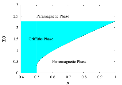
Figure 1: Phase diagram of the two-dimensional bond diluted Ising ferromagnet in the $p$-$T$ plane. The shaded region is called the Griffiths phase.

According to the argument by Griffiths [14], the free energy of the random bond Ising ferromagnet must be a non-analytic function of the external field $h$ in the temperature regime above the transition temperature $T_{c}(p)$ and below $T_{c}(p=1)$ of corresponding non-diluted system. The free energy has an essential singularity as a function of $h$ in the zero $h$ limit, which is refereed to as Griffiths singularity. Physically, the Griffiths singularity is related with the existence of arbitrarily large compact clusters in which most of the interactions take $J$. The probability of the existence of such large clusters is suppressed exponentially in their size and the contribution of such clusters to the susceptibility is proportional to the size at low temperatures. This means that the arbitrarily large clusters have rare but significantly important effect leading to the Griffiths singularity. However, the singularity of the free energy is believed to be too weak to find in experiments and numerical simulations. Meanwhile, such large clusters have also important consequences for dynamical properties because they flip from one to the other stable states very slowly at low temperatures. In fact, many theoretical [21, 22, 23] and numerical [24, 25] studies have found that time correlation functions in the temperature regime $T_{c}(p)<T<T_{c}(p=1)$ exhibit non-exponential slow relaxation which is not expected in the simple paramagnetic phase. Thus, the temperature regime lying between $T_{c}(p)$ and $T_{c}(p=1)$ is called the Griffiths phase.

Figure 2: Schematic pictures of the distribution of the inverse susceptibility for a random bond Ising model. (a) At $T>T_{c}(p=1)$, the distribution is bounded. (b) In the Griffiths phase at $T_{c}(p)<T<T_{c}(p=1)$, the smallest edge of the distribution reaches the origin. (c) At the transition temperature $T=T_{c}(p)$, the statistical weight near the origin is significant and the average of the susceptibility diverges.

In this work, we study the distribution of the (inverse) susceptibility $\chi$ at finite temperatures. We consider that the distribution of the susceptibility could be used as an indicator of the Griffiths singularity on the analogy of the Bray-Moore argument [26] in which the density of states of the inverse susceptibility matrix is discussed. As is sketched in figure 2, the distribution of the inverse susceptibility $P(\chi^{-1})$ is bounded at high temperatures and as the temperature decreases the edge of the distribution touches the origin without statistical weight. We regard this feature of the distribution as the Griffiths singularity. Using the MC algorithm described in the previous section with setting $\langle A\rangle=\chi^{-1}$, we evaluate the distribution of the inverse susceptibility numerically near the origin in the Griffiths phase.

4 Application of the importance-sampling algorithm

We perform the importance-sampling MC simulation for sampling the interaction bonds $\mathbf{J}$. In the inner loop of the step (ii) in section 2 we have to calculate the bulk susceptibility for a given $\mathbf{J}$, which is expressed in disordered phase as

$$\chi(\mathbf{J})=\frac{1}{N}\left\langle\left(\sum_{i}S_{i}\right)^{2}\right\rangle.$$ (10)

For unfrustrated spin systems, cluster MC algorithms are known to be quite efficient for reducing critical slowing down near phase transitions [27, 28]. Furthermore, some physical quantities can be calculated using an improved estimator expressed in terms of clusters, which makes statistical error reduced substantially. The improved estimator for the susceptibility is given by the mean squared cluster size in the Swendsen-Wang cluster algorithm. Using the cluster MC algorithm with the improved estimator [27], the susceptibility of the model is calculated with sufficient accuracy.

We firstly perform the simple-sampling algorithm for $10^{3}\sim 10^{4}$ independent interaction bonds and obtain a first guess for the guiding function $\tilde{P}(\chi^{-1})$. Starting from an initial configuration of the interaction bonds randomly set to $J$ with the probability $p$ and $0$ with $1-p$, we choose a small percentage of the total bonds at random, and generate a new candidate for the interaction bonds by refreshing the chosen bonds with the same probability $p$. For the new candidate, we calculate the susceptibility by the method mentioned above and accept it with the probability of equation (5), in which a working guiding function $\tilde{P}(\chi^{-1})$ is used and also update by the step (iii) in section 2. Because we are interested in the behavior of $P(\chi^{-1})$ near th origin and not in $P(\chi^{-1})$ with a large value of $\chi^{-1}$, we put bounds to the maximum value of $\chi^{-1}$ allowed in the simulation by $[\chi^{-1}]+3\sigma$ with $\sigma$ being the standard deviation, which is roughly estimated in the preliminary simple-sampling run. In actual simulation, a new candidate with the value beyond the limit is rejected with probability one.

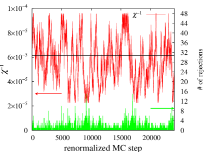
Figure 3: A Monte Carlo trajectory of the value of $\chi^{-1}$ of the two-dimensional bond-diluted Ising model for $L=32$, $p=0.6$ and $T/J=1.5$. The horizontal axis means renormalized MC steps which are incremented by one when a new value of $\chi^{-1}$ is accepted. The value of $\chi^{-1}$ as a function of the MC step is represented by the straight line and the number of rejections at the MC step is given by bar chart.

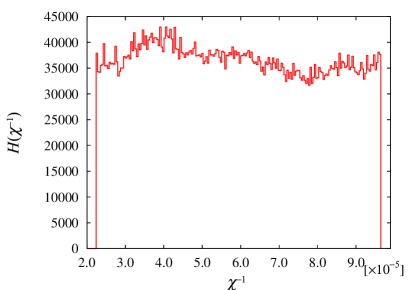
Figure 4: Histogram of the inverse susceptibility obtained by an importance sampling algorithm of the two-dimensional bond-diluted Ising model. The parameters used in the simulation is the same as those in figure 4.

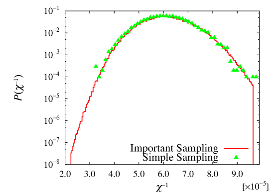
Figure 5: Distribution of the inverse susceptibility of the two-dimensional bond-diluted Ising model with $p=0.6$ for $L=32$ and $T/J=1.5$. The solid line represents $P(\chi^{-1})$ obtained by the importance-sampling MC, and the triangles are that by the simple sampling.

Figure 4 shows an example of Monte Carlo trajectory of the value of $\chi^{-1}$ for linear size $L=32$, $p=0.6$ and $T/J=1.5$ and figure 4 shows the histogram of the inverse susceptibility in this simulation. It is found that the importance-sampling MC simulation can cover a wide range of $\chi^{-1}$. The re-weighted distribution by the guiding function with equation (8) and also the simple-sampling histogram for comparison are shown in figure 5. We see that the resolution in the simple-sampling result determined by the number of samplings is largely improved by the use of the importance sampling which leads to probabilities of order $10^{-8}$.

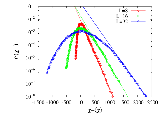
Figure 6: Distribution functions of the inverse susceptibility as a function of $1/\chi^{-1}$ of the two-dimensional bond-diluted Ising model with $p=0.6$ and $T/J=2.0$. The system sizes are $N=8^{2}(\opentriangledown)$, $16^{2}(\opendiamond)$ and $32^{2}(\opentriangle)$. The straight lines are the fitting result of the exponential function $p(\chi^{-1})=B\exp(-C/\chi^{-1})$ with $B$ and $C$ being fitting parameters.

We have calculated the inverse-susceptibility distributions with $L=8$, $16$, $32$, (and $64$ for some cases) at a few temperatures in the Griffiths and paramagnetic phases. In the paramagnetic phase above $T_{c}(p=1)$, the distribution functions of the inverse susceptibility are scaled well as a function of $X=(\chi-\chi_{0})/\sigma$ with $\chi_{0}$ and $\sigma$ being the average and the standard deviation, respectively(not shown here), and the scaling function is well described as a Gaussian. Figure 6 shows the distribution as a function of $1/\chi^{-1}$ in the Griffiths phase with $p=0.6$ and $T/J=2.0$. In contrast to that in the paramagnetic phase, the distribution has an exponential tail for large $\chi$

$$P(\chi^{-1})\sim\exp(-C/\chi^{-1}),$$ (11)

where $C$ is a temperature dependent parameter. This behavior is also described by the exponential tail of a Gumbel distribution. The parameter $C$ is obtained by fitting the function form of equation (11) for large $\chi$ to the data for each size and temperature. The fitting result for $C$ has still size dependence. We thus extract the thermodynamic value by fitting a polynomial function of $1/L$ to the value of $C$. The temperature dependent of the extrapolated value of $C$ for the exponential tail is shown in figure 7. In general [26], we expect that the parameter $C$ vanishes as $T$ goes to $T_{c}(p)$ from above since $P(\chi^{-1})$ should be a power law of $\chi^{-1}$ for $T=T_{c}(p)$, while $C$ diverges as $T$ goes to $T_{c}(p=1)$ since $P(\chi^{-1})$ should have a gap from the origin $\chi^{-1}=0$ for $T>T_{c}(p=1)$. Our result shown in figure 7 is consistent with this argument although further studies would be necessary to confirm the conclusion. It would be interested to see the precise functional form of $C$ near $T_{c}(p)$ and $T_{c}(p=1)$.

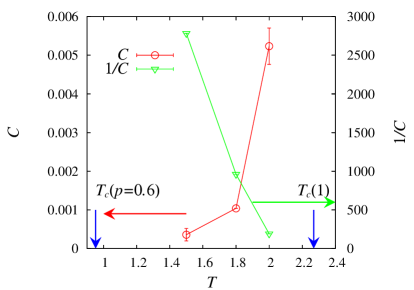
Figure 7: Temperature dependence of the parameter $C$ for the left axis and $1/C$ for the right.

5 Conclusions and perspectives

In summary, we have developed an importance-sampling MC algorithm for quenched disordered systems originally proposed in references [15, 16]. The algorithm discussed is an efficient sampling method with appropriate weight for the quenched variables, which, for instance, correspond to the interaction bonds in random spin systems, while most of simulations have so far used a simple-sampling method in which the quenched variables are generated by a given probability distribution. Reference [16] suggested that a learning procedure could be simplified by introducing a given guiding function as the weight for sampling the quenched variables. In this work, we explicitly formulate the learning procedure of the weight using the multicanonical method [4] combined with Wang-Landau recursion [19, 20]. Because the method explained in this paper does not assume a priori knowledge of the weight, it could be complementary to the method in reference [16] for studying a wide class of quenched random systems. It should be noted that the method can be applied to finite-temperature calculation of any distribution of observables as demonstrated in this work, while the applications are limited to ground-state-energy distribution previously. For example, the method can be in principle applicable to distribution functions of relaxation time and/or solving time for randomly constraint satisfaction problems.

We have applied the algorithm to evaluate the distribution of the susceptibility in a two-dimensional bond-diluted Ising model which concerns the so-called Griffiths singularity. We have found that the distribution has an exponential tail for large value of the susceptibility and that the evaluated slope of the exponential tail exhibits significant temperature dependence in the Griffiths phase which is consistent with a simple argument [26]. It would be interesting to confirm the Griffiths singularity in spin-glass systems. Then, the cluster MC method used in the inner-loop calculation for taking an average over spin variables should be replaced by an extended-ensemble based MC method [3] because it does not work efficiently in frustrated spin systems such as spin glasses. This would require relatively extensive computational time but it would be helpful to use massively parallel simulations for the Wang-Landau recursion in our method .

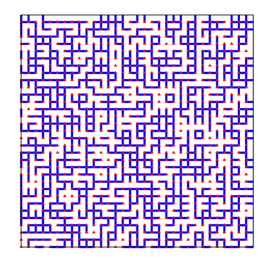
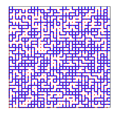
Figure 8: Examples of interaction bonds of the two-dimensional bond-diluted Ising model for $L=32$, $p=0.6$ and $T/J=1.5$. Triangles are sites of square lattice that the spins are defined on. The blue lines represent the interaction bonds with $J$ between the nearest neighbor spins. The left viewgraph is an sample with $\chi^{-1}=9.67\times 10^{-5}$, and the right one shows a rare sample with the smallest value of $\chi^{-1}=2.24\times 10^{-5}$ in our simulations. See also the distribution $P(\chi^{-1})$ in figure 5. It would be found that the right one is more dense and more compact than the left one.

The importance-sampling MC method discussed in this paper is also regarded as a sampling method of rare events as originally pointed out in reference [15]. A direct application in this respect is to see rare samples which occur very unlikely. Figures 8 show two rare examples of interaction bonds found in our simulations of the bond-diluted Ising model. This makes possible further research on the nature of such rare samples, for example fractal properties not discussed here, which causes the large susceptibility and the Griffiths singularity. This method could be generally useful as an experimental tool for picking up the rare events and for studying their properties.

We would like to thank A. P. Young and H. G. Katzgraber for fruitful discussions. This work was supported by the Grants-In-Aid for Scientific Research (No. 17540348 and No. 18079004) from MEXT of Japan. Part of the numerical simulations were partially performed on the SGI Origin 2800/384 at the Supercomputer Center, ISSP, the University at Tokyo.

References

References

- [1] Binder K and Landau D P 2000 A guide to Monte Carlo simulations in statistical physics (Cambridge: Cambridge University Press)
- [2] Liu J S 2001 Monte Carlo strategies in scientific computing (New York: Springer-Verlag)
- [3] For a review of the extended ensemble MC method, Iba Y 2001 Int. J. Mod. Phys. C 12 623
- [4] Berg B A and Neuhaus T 1992 Phys. Rev. Lett. 68 9
- [5] Marinari E and Parisi G 1992 Europhys. Lett. 19 451
- [6] Hukushima K and Nemoto K 1996 J. Phys. Soc. Jpn. 65 1604
- [7] Binder K and Young A P 1986 Rev. Mod. Phys. 58 801
- [8] Mézard M, Parisi G and Virasoro M A 1987 Spin glass theory and Beyond (Singapore: World Scientific)
- [9] Young A P 1997 Spin glasses and random fields ( Singapore : World Scientific)
- [10] Kawashima N and Rieger H 2004 Frustrated Spin Systems ed H T Diep (Singapore : World Scientific) chapter 9 pp 491 (Preprint cond-mat/0312432)
- [11] Hilfer R, Biswal B, Mattutis H G and Janke W 2003 Phys. Rev. E 68 046123
- [12] Bouchaud J P, Krzakala F and Martin O C 2003 Phys. Rev. B 68 224404
- [13] Katzbraber H G, Körner M, Liers F, Jünger M and Hartmann A K 2005 Phys. Rev. B 72 094421
- [14] Griffiths R B 1969 Phys. Rev. Lett. 23 17
- [15] Hartmann A K 2002 Phys. Rev. E 65 056102
- [16] Körner M, Katzgraber H G and Hartmann A K 2006 J. Stat. Mech.: Theory Exp. P04005
- [17] Monthus C and Garel T 2006 Phys. Rev. E 74 051109
- [18] Iba Y and Hukushima K 2007 Preprint arXiv:0709.2578
- [19] Wang F and Landau D P 2001 Phys. Rev. Lett. 86 2050
- [20] Wang F and Landau D P 2001 Phys. Rev. E 64 056101
- [21] Dhar D, Randeria M and Sethna J P 1988 Europhys. Lett. 5 485
- [22] Bray A J 1987 Phys. Rev. Lett. 59 586
- [23] Bray A J 1988 Phys. Rev. Lett. 60 720
- [24] Takano H and Miyashita S 1989 J. Phys. Soc. Jpn. 58 3871
- [25] Colborne S G W and Bray A J 1989 J. Phys. A: Math. Gen. 22 2505
- [26] Bray A J and Moore M A 1982 J. Phys. C: Solid State Phys. 15 L765
- [27] Swendsen R H and Wang J-S 1987 Phys. Rev. Lett. 58 86
- [28] Wolff U 1989 Phys. Rev. Lett. 62 361