Abstract

The gauge threshold corrections for globally consistent $\mathbb{Z}_{2}\times\mathbb{Z}^{\prime}_{2}$ orientifolds with rigid intersecting D6-branes are computed. The one-loop corrections to the holomorphic gauge kinetic function are extracted and the Kähler metrics for the charged chiral multiplets are determined up to two constants.

1 Introduction and Motivation

Gauge threshold corrections in D-brane models [1, 2, 3, 4, 5] have lately attracted renewed interest. This is mainly due to the fact that they were shown to be equal to one-loop amplitudes appearing in superpotential couplings generated by euclidean D-brane instantons [6, 7]. As the gauge threshold corrections generically are not holomorphic functions of the moduli fields, it is not a priori clear how these couplings can be incorporated in a superpotential. It can however be shown that a cancellation between the non-holomorphic terms in the thresholds and terms arising from non-trivial, moduli-dependent Kähler metrics takes place, thus rendering both the instanton-generated superpotential and the one-loop corrected gauge kinetic function holomorphic [8, 9, 10].

Gauge threshold corrections in D6-brane models on toroidal backgrounds have so far only been computed for so-called bulk branes, which are uncharged under twisted sector RR-fields [11, 12]. Here the prototype example is the $\mathbb{Z}_{2}\times\mathbb{Z}_{2}$ orbifold with $h_{21}=3$, which only has eight three-cycles, all of which are bulk cycles. Twisted three-cycles occur for the $\mathbb{Z}_{2}\times\mathbb{Z}^{\prime}_{2}$ orbifold with $h_{21}=51$. This orbifold is a particularly interesting background for intersecting D6-brane models because the CFT is free and thus explicit calculations can be performed and, most strikingly, there exist rigid three-cycles. These latter ones allow one to construct models without phenomenologically undesirable adjoint fields and therefore, in particular, asymptotically free gauge theories [16]. Moreover, these rigid cycles are important when studying non-perturbative effects because euclidean D2-brane (short E2-brane) instantons wrapping these cycles have the zero mode structure needed for a contribution to the superpotential [17, 18]. This means that, due to the aforementioned relation between one-loop threshold corrections and the one-loop instanton amplitudes, the results of this paper are relevant when determining E2-instanton effects in toroidal intersecting D6-brane models.

In this paper, gauge threshold corrections for D6-brane models on the $\mathbb{Z}_{2}\times\mathbb{Z}^{\prime}_{2}$ orbifold with $h_{21}=51$ [16], in which branes can be charged under the twisted RR fields, are computed. Furthermore, it is shown that also on this background a cancellation between the non-holomorphic parts of the gauge thresholds and the terms involving the Kähler metrics occurs in an equation relating the holomorphic gauge kinetic function to the physical gauge coupling, which is the one calculated in string theory. Since the main body of this paper is quite technical, let us mention two of our main findings. A summary of all the results including formulas is given at the end of the paper. We will determine the one-loop corrections to the holomorphic gauge kinetic function $f_{a}$ for the gauge theory on a brane stack labelled $a$. It is interesting to see that on this background, in contradistinction to the case of the $\mathbb{Z}_{2}\times\mathbb{Z}_{2}$ orbifold with $h_{21}=3$ [8], there are corrections to the gauge kinetic function from sectors preserving $\mathcal{N}=1$ supersymmetry.

The gauge threshold corrections computed in this paper allow for a determination of Kähler metrics of charged matter on the background considered. The metric for the vector-like bifundamental matter arising from strings stretched between two stacks of branes that are coincident but differ in their twisted charges can be determined using holomorphy arguments and yields the expected results. Equivalently, one can determine, up to two constants, the Kähler metric for the chiral bifundamental matter arising at the intersection of two stacks of branes, confirming previous findings.

The results of this paper extend those computed in the T-dual picture [9, 10] insofar as to be valid in a global rather than local model and to include more general twisted sector charges. In addition, a new contribution to the so-called universal gauge coupling corrections [19, 20, 21, 8] is found. Their appearance, together with the holomorphy of the gauge kinetic function, implies a redefinition of the twisted complex structure moduli at one loop.

Before we dwell upon the technical details of our computation, let us spell out the motivation for this project, which is twofold. Firstly, the gauge threshold corrections are computed. They are important in D-brane models as the gauge couplings on different branes depend on the volumes of the cycles the branes wrap and therefore are generically not equal at the compactification or string scale. This poses a potential problem with the apparent gauge coupling unification seen in the MSSM which could be solved upon taking the gauge threshold corrections into account.

Secondly, as already mentioned, the present background allows for E2-instanton contributions to the superpotential and is thus a good arena to explicitly study non-perturbative effects in intersecting D6-brane models. Examples of such effects that are important are Majorana mass terms for the right-handed neutrinos [18, 22] and the issue of moduli stabilisation [23]. Note in this context that the one-loop corrections determined here lead to a dependence of the instanton-induced terms on the Kähler moduli, whereas, at tree level, they only depend on the complex structure moduli.

2 Setup and partition functions

The setup considered in this paper [16] is an orientifold of an orbifolded torus. The torus is a factorisable six-torus $T^{6}=T^{2}\times T^{2}\times T^{2}$ and the orbifold group is $\mathbb{Z}_{2}\times\mathbb{Z}^{\prime}_{2}$, where each $\mathbb{Z}_{2}$-factor inverts two two-tori. There are three $\mathbb{Z}_{2}$-twisted sectors with sixteen fixed points each. The orientifold group is $\Omega R(-1)^{F_{L}}$, where $\Omega$ is world-sheet parity, $R$ an antiholomorphic involution and $F_{L}$ the left-moving spacetime fermion number. The three two-tori have radii $R_{1,2}^{(i)}$ along the $x^{i}$,$y^{i}$-axes, $i\in\{1,2,3\}$. The tori may ($\beta^{i}=1/2$) or may not ($\beta^{i}=0$) be tilted. There are four orbifold fixed points on each torus, at $(0,0)$, $(0,R_{2}^{(i)}/2)$, $(R_{1}^{(i)}/2,\beta^{i}R_{2}^{(i)}/2)$ and $(R_{1}^{(i)}/2,(1+\beta^{i})R_{2}^{(i)}/2)$. They will be labelled fixed points 1,2,3 and 4. All this geometrical data is shown in figure 1 for an untilted and a tilted torus.

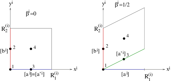
Figure 1: Geometry of the two-tori, orbifold fixed points and one-cycles

(Stacks of) D-branes on this background are described by the wrapping numbers $(n^{i},m^{i})$, the charges under the twisted RR-fields $\epsilon^{i}\in\{-1,1\}$, the position $\delta^{i}\in\{0,1\}$ and the discrete Wilson lines $\lambda^{i}\in\{0,1\}$. The brane wraps the one-cycle $n^{i}[{a^{\prime}}^{i}]+m^{i}[b^{i}]$ on the $i$’th torus, the fundamental one-cycles $[{a^{\prime}}^{i}]=[a^{i}]+\beta^{i}[b^{i}]$ and $[b^{i}]$ are shown in figure 1. The $\epsilon^{i}$ satisfy $\epsilon^{1}=\epsilon^{2}\epsilon^{3}$. The position is described by the three parameters $\delta^{i}$, where $\delta^{i}=0$ if the brane goes through fixed point 1 on the i’th torus and $\delta^{i}=1$ otherwise. An alternative way to characterise a brane is to use $\epsilon^{i}_{kl}\in\{-1,0,1\}$, $i\in\{1,2,3\}$, $k,l\in\{1,2,3,4\}$ [16], instead of $\epsilon^{i}$, $\delta^{i}$ and $\lambda^{i}$. $\epsilon^{i}_{kl}$ is the charge of the brane under the fixed point labelled $kl$ in the $i$’th twisted sector. The $\epsilon^{i}_{kl}$ can be determined from $\epsilon^{i}$, $\delta^{i}$ and $\lambda^{i}$. Note that for each $i$ only four out of the sixteen $\epsilon^{i}_{kl}$ are non-zero. In both these descriptions there is some redundancy [16]. Rather than fixing some of the $\epsilon^{i}_{kl}$ charges to be 1 [16], it will here be more convenient to choose $n^{1,2}>0$ (or $m^{i}$ positive if $n^{i}$ vanishes).

It is useful to define $\widetilde{m}^{i}=m^{i}+\beta^{i}n^{i}$, such that a brane wraps the one-cycle $n^{i}[a^{i}]+\widetilde{m}^{i}[b^{i}]$ on the $i$’th torus. The volume of this one-cycle is given by

$$V^{i}=\sqrt{(n^{i})^{2}(R_{1}^{(i)})^{2}+(\widetilde{m}^{i})^{2}(R_{2}^{(i)})^{2}}$$ (2.1)

and the tree-level gauge coupling reads:

$$\frac{1}{g_{tree}^{2}}=e^{-\phi_{10}}\prod_{i}V^{i}=\frac{e^{-\phi_{4}}}{(T_{1}T_{2}T_{3})^{1/2}}\prod_{i}V^{i}=\frac{(SU_{1}U_{2}U_{3})^{1/4}}{(T_{1}T_{2}T_{3})^{1/2}}\prod_{i}V^{i}\,.$$ (2.2)

Here, $\phi_{10}$($\phi_{4}$) is the 10(4)-dimensional dilaton in string frame, $S$ is the dilaton in Einstein frame, $U_{i}$ are the (real parts of the) complex structure moduli in Einstein frame and $T_{i}=R_{1}^{(i)}R_{2}^{(i)}$ are the (real parts of the) Kähler moduli. From (2.2) one can, using the supersymmetry condition (see below), derive the dependence of the tree-level gauge kinetic function on the untwisted moduli [24]:

$$\hat{f}_{tree}=S^{c}n^{1}n^{2}n^{3}-\sum_{i\neq j\neq k=1}^{3}U_{i}^{c}n^{i}\widetilde{m}^{j}\widetilde{m}^{k}\,.$$ (2.3)

$S^{c}$ and $U_{i}^{c}$ are the complexified dilaton and complex structure moduli, the axions being RR-fields. Similarly, $T^{c}_{i}$ are complexified Kähler moduli, the axions stemming from the NSNS 2-form-field.

The D-brane is rotated by the angles $\theta^{i}$, defined via $\tan\theta^{i}=\widetilde{m}^{i}R_{2}^{(i)}/n^{i}R_{1}^{(i)}$, with respect to the x-axes of the three tori. Only supersymmetric configurations will be considered in this paper, i.e. $\sum_{i=1}^{3}\theta^{i}=0$.

The charges of the four orientifold planes are denoted $\eta_{\Omega R}$ and $\eta_{\Omega Ri}$, $i\in\{1,2,3\}$ and have to satisfy

$$\eta_{\Omega R}\prod_{i=1}^{3}\eta_{\Omega Ri}=-1$$ (2.4)

in the present case of the $\mathbb{Z}_{2}\times\mathbb{Z}^{\prime}_{2}$ orbifold with $h_{21}=51$ [16]. The tadpole cancellation conditions are given by

$$\sum_{a}N_{a}n_{a}^{1}n_{a}^{2}n_{a}^{3}=16\eta_{\Omega R}$$ (2.5)

$$\sum_{a}N_{a}n_{a}^{i}\widetilde{m}_{a}^{j}\widetilde{m}_{a}^{k}=-2^{4-2\beta^{j}-2\beta^{k}}\eta_{\Omega Ri}\qquad i\neq j\neq k\in\{1,2,3\}$$ (2.6)

$$\sum_{a}N_{a}n_{a}^{i}(\epsilon_{a,kl}^{i}-\eta_{\Omega R}\eta_{\Omega Ri}\epsilon_{a,R(k)R(l)}^{i})=0$$ (2.7)

$$\sum_{a}N_{a}\widetilde{m}_{a}^{i}(\epsilon_{a,kl}^{i}+\eta_{\Omega R}\eta_{\Omega Ri}\epsilon_{a,R(k)R(l)}^{i})=0,$$ (2.8)

where $R(k)=k$ in case of an untilted torus and $R(\{1,2,3,4\})=\{1,2,4,3\}$ in the other case [16] and the sum is a sum over all stacks of branes. $N_{a}$ denotes the number of branes on stack $a$. The wrapping numbers and twisted charges carry an index $a$ denoting the brane stack which they describe. The orientifold projection acts on the wrapping numbers and twisted charges as follows:

$$\widetilde{m}^{I} \rightarrow -\widetilde{m}^{I}$$ (2.9)

$$\epsilon_{kl}^{i} \rightarrow -\eta_{\Omega R}\eta_{\Omega Ri}\epsilon^{i}_{R(k)R(l)}\,.$$ (2.10)

The massless open string spectrum can be read of from the open string partition function given by annulus (and Möbius) amplitudes without any vertex operators inserted. These can be calculated from boundary (and crosscap) states describing the D-branes (and O-planes) [25, 26, 27, 28, 29, 30, 31]. Only the annulus amplitudes will be given here, and four cases will be distinguished (These are not all possibilities there are, but all needed here.), that will also be important in the rest of this paper:

Case 1:

The annulus has both boundaries on the same stack of branes $a$. The amplitude is

$$\mathcal{A}_{aa}^{(1)} = -N_{a}^{2}\int_{0}^{\infty}dl\Bigg{[}\frac{\vartheta_{3}^{4}-\vartheta_{4}^{4}-\vartheta_{2}^{4}+\vartheta_{1}^{4}}{\eta^{12}}\prod_{i=1}^{3}\frac{(V_{a}^{i})^{2}}{R_{1}^{(i)}R_{2}^{(i)}}\widetilde{L}_{aa}^{(i)}$$ (2.11)

$$+16\sum_{i=1}^{3}\sigma_{aa}^{i}\frac{\vartheta_{3}^{2}\vartheta_{2}^{2}-\vartheta_{4}^{2}\vartheta_{1}^{2}-\vartheta_{2}^{2}\vartheta_{3}^{2}+\vartheta_{1}^{2}\vartheta_{4}^{2}}{\eta^{6}\vartheta_{4}^{2}}\frac{(V_{a}^{i})^{2}}{R_{1}^{(i)}R_{2}^{(i)}}\widetilde{L}_{aa}^{(i)}\Bigg{]},$$

where $\sigma_{ab}^{i}=\frac{1}{4}\sum_{k,l=1}^{4}\epsilon^{i}_{a,kl}\epsilon^{i}_{b,kl}$, $\vartheta=\vartheta(0,2il)$, $\eta=\eta(2il)$ and $V_{a}^{i}$, defined in (2.1), now carries an index $a$ to denote the brane stack considered. The following Kaluza-Klein and winding sum has been defined [32]:

$$\widetilde{L}_{ab}^{(i)} = \sum_{m,w}\exp\left[-\pi l(V_{a}^{i})^{2}\left(\frac{m^{2}}{(R_{1}^{(i)}R_{2}^{(i)})^{2}}+w^{2}\right)+i\pi m(\delta_{a}^{i}-\delta_{b}^{i})+i\pi w(\lambda_{a}^{i}-\lambda_{b}^{i})\right]$$

Case 2:

The annulus stretches between two stacks of D-branes $a$ and $b$ wrapping the same submanifold of the covering six-torus of the internal space and having the same discrete Wilson lines turned on($\lambda_{a}^{i}=\lambda_{b}^{i}$). This means in particular $\theta_{a}^{i}=\theta_{b}^{i}$,$V_{a}^{i}=V_{b}^{i},\delta_{a}^{i}=\delta_{b}^{i}$, however not all twisted charges $\epsilon^{i}$ are equal.

One can show that in this case $\sigma_{ab}^{i}=\pm 1$. The amplitude is

$$\mathcal{A}_{ab}^{(2)} = -N_{a}N_{b}\int_{0}^{\infty}dl\Bigg{[}\frac{\vartheta_{3}^{4}-\vartheta_{4}^{4}-\vartheta_{2}^{4}+\vartheta_{1}^{4}}{\eta^{12}}\prod_{i=1}^{3}\frac{(V_{a}^{i})^{2}}{R_{1}^{(i)}R_{2}^{(i)}}\widetilde{L}_{ab}^{(i)}$$ (2.12)

$$+16\sum_{i=1}^{3}\sigma_{ab}^{i}\frac{\vartheta_{3}^{2}\vartheta_{2}^{2}-\vartheta_{4}^{2}\vartheta_{1}^{2}-\vartheta_{2}^{2}\vartheta_{3}^{2}+\vartheta_{1}^{2}\vartheta_{4}^{2}}{\eta^{6}\vartheta_{4}^{2}}\frac{(V_{a}^{i})^{2}}{R_{1}^{(i)}R_{2}^{(i)}}\widetilde{L}_{ab}^{(i)}\Bigg{]}.$$

Case 3:

The two stacks of branes wrap submanifolds that are homologically equal on the covering torus (This implies $\theta_{a}^{i}=\theta_{b}^{i}$,$V_{a}^{i}=V_{b}^{i}$.), but do not satisfy $\lambda_{a}^{i}=\lambda_{b}^{i}$, $\delta_{a}^{i}=\delta_{b}^{i}$ for all $i$. The amplitude looks as the one of case 2.

Case 4:

The annulus stretches between two branes that intersect at non-trivial angles on all three tori. The amplitude reads

$$\mathcal{A}_{ab}^{(4)}=N_{a}N_{b}\int_{0}^{\infty}dl\Bigg{[}8\left({\textstyle\prod_{i=1}^{3}I_{ab}^{i}}\right)\sum_{\alpha,\beta}(-1)^{2(\alpha+\beta)}\frac{\vartheta\genfrac{[}{]}{0.0pt}{}{\alpha}{\beta}(0)}{\eta^{3}}\prod_{i=1}^{3}\frac{\vartheta\genfrac{[}{]}{0.0pt}{}{\alpha}{\beta}(\theta_{ab}^{i})}{\vartheta\genfrac{[}{]}{0.0pt}{}{1/2}{1/2}(\theta_{ab}^{i})}$$ (2.13)

$$+32\sum_{i\neq j\neq k}I_{ab}^{i}\,\sigma_{ab}^{i}\sum_{\alpha,\beta}(-1)^{2(\alpha+\beta)}\frac{\vartheta\genfrac{[}{]}{0.0pt}{}{\alpha}{\beta}(0)}{\eta^{3}}\frac{\vartheta\genfrac{[}{]}{0.0pt}{}{\alpha}{\beta}(\theta_{ab}^{i})}{\vartheta\genfrac{[}{]}{0.0pt}{}{1/2}{1/2}(\theta_{ab}^{i})}\frac{\vartheta\genfrac{[}{]}{0.0pt}{}{|\alpha-1/2|}{\beta}(\theta_{ab}^{j})}{\vartheta\genfrac{[}{]}{0.0pt}{}{0}{1/2}(\theta_{ab}^{j})}\frac{\vartheta\genfrac{[}{]}{0.0pt}{}{|\alpha-1/2|}{\beta}(\theta_{ab}^{k})}{\vartheta\genfrac{[}{]}{0.0pt}{}{0}{1/2}(\theta_{ab}^{k})}\Bigg{]},$$

where $\theta_{ab}^{i}=\theta_{a}^{i}-\theta_{b}^{i}$ and the intersection number $I_{ab}^{i}=(\widetilde{m}_{a}^{i}n_{b}^{i}-\widetilde{m}_{b}^{i}n_{a}^{i})$ were defined.

Upon transforming into the open string channel, one finds the following massless spectrum: Case 1 yields a massless vector multiplet in the adjoint representation of $U(N_{a})$. Case 2 gives a massless hypermultiplet in the bifundamental representation of $U(N_{a})\times U(N_{b})$. In case 3 there are no massless fields. In case 4 one finds $|\Upsilon_{ab}|$, $\Upsilon_{ab}=\frac{1}{4}\prod_{i=1}^{3}I_{ab}^{i}+\sum_{i=1}^{3}I_{ab}^{i}\sigma_{ab}^{i}$, chiral multiplets in the bifundamental representation of $U(N_{a})\times U(N_{b})$.

3 Gauge threshold corrections

The gauge threshold corrections will be computed using the background field method employed previously [33, 34, 11]. This means that the one-loop correction to the gauge coupling of brane $a$ induced by brane $b$ is determined as follows. First, one replaces the 4d spacetime part of the partition function in the above expression as follows [11]:

$$\frac{\vartheta\genfrac{[}{]}{0.0pt}{}{\alpha}{\beta}(0,2il)}{\eta^{3}(2il)}\rightarrow 2i\pi Bq_{a}\frac{\vartheta\genfrac{[}{]}{0.0pt}{}{\alpha}{\beta}(-\epsilon_{a},2il)}{\vartheta\genfrac{[}{]}{0.0pt}{}{1/2}{1/2}(-\epsilon_{a},2il)},$$ (3.1)

where $\pi\epsilon_{a}=\arctan(\pi q_{a}B)$, $q_{a}$ is the charge of the open string ending on brane $a$ and $B$ is the background magnetic field in the 4d spacetime. One then expands the resulting expressions in a series in $B$ and the coefficient of $B^{2}$ gives the desired expression for the correction to the gauge coupling, which needs to be evaluated further.

For the four cases distinguished above one finds, denoting the amplitudes after the manipulations described with an additional superscript $g$:

$$\mathcal{A}_{aa}^{g(1)} = 32\pi\,N_{a}^{2}\int_{0}^{\infty}dl\sum_{i=1}^{3}\sigma_{aa}^{i}\frac{(V_{a}^{i})^{2}}{R_{1}^{(i)}R_{2}^{(i)}}\widetilde{L}_{aa}^{(i)}$$ (3.2)

$$\mathcal{A}_{ab}^{g(2)} = 32\pi\,N_{a}N_{b}\int_{0}^{\infty}dl\sum_{i=1}^{3}\sigma_{ab}^{i}\frac{(V_{a}^{i})^{2}}{R_{1}^{(i)}R_{2}^{(i)}}\widetilde{L}_{ab}^{(i)}$$ (3.3)

$$\mathcal{A}_{ab}^{g(3)} = 32\pi\,N_{a}N_{b}\int_{0}^{\infty}dl\sum_{i=1}^{3}\sigma_{ab}^{i}\frac{(V_{a}^{i})^{2}}{R_{1}^{(i)}R_{2}^{(i)}}\widetilde{L}_{ab}^{(i)}$$ (3.4)

$$\mathcal{A}_{ab}^{g(4)} = N_{a}N_{b}\int_{0}^{\infty}dl\Bigg{[}8\left({\textstyle\prod_{i=1}^{3}I_{ab}^{i}}\right)\,\sum_{i=1}^{3}\frac{\vartheta^{\prime}_{1}(\theta_{ab}^{i},2il)}{\vartheta_{1}(\theta_{ab}^{i},2il)}+\sum_{i\neq j\neq k}32I_{ab}^{i}\,\sigma_{ab}^{i}$$ (3.5)

$$\left(\frac{\vartheta^{\prime}_{1}(\theta_{ab}^{i},2il)}{\vartheta_{1}(\theta_{ab}^{i},2il)}+\frac{\vartheta^{\prime}_{4}(\theta_{ab}^{j},2il)}{\vartheta_{4}(\theta_{ab}^{j},2il)}+\frac{\vartheta^{\prime}_{4}(\theta_{ab}^{k},2il)}{\vartheta_{4}(\theta_{ab}^{k},2il)}\right)\Bigg{]}.$$

The overall normalisation will later be fixed by demanding the running of the gauge coupling with the correct beta function coefficient, but the relative normalisation is taken into account correctly. The full correction to the gauge coupling on brane $a$ is given by summing over all annuli (and Möbii) with at least one boundary on brane $a$.

The above expressions can be evaluated analogously to the corresponding ones in the $\mathbb{Z}_{2}\times\mathbb{Z}_{2}$ orbifold with $h_{21}=3$ [11, 12]. The results are:

$$\mathcal{A}_{aa}^{g(1)} = 32\pi\,N_{a}^{2}\int_{0}^{\infty}dl\sum_{i=1}^{3}\sigma_{aa}^{i}\frac{(V_{a}^{i})^{2}}{R_{1}^{(i)}R_{2}^{(i)}}$$ (3.9)

$$+32\pi\,N_{a}^{2}\left(\sigma_{aa}\ln\left[\frac{M_{s}^{2}}{\mu^{2}}\right]-\sum_{i=1}^{3}\sigma_{aa}^{i}\ln\left[(V_{a}^{i})^{2}\right]\right)$$

$$-32\pi\,N_{a}^{2}\sum_{i=1}^{3}4\,\sigma_{aa}^{i}\,\ln\left[\eta(iR_{1}^{(i)}R_{2}^{(i)})\right]$$

$$-32\pi\,N_{a}^{2}\sigma_{aa}\ln[4\pi]\,.$$

Here, $\sigma_{ab}=\sum_{i=1}^{3}\sigma_{ab}^{i}$ was defined and the divergence $\int^{\infty}\frac{dt}{t}$ arising from the massless open string modes was replaced by $\ln\left[M_{s}^{2}/\mu^{2}\right]$ [12]. For the cases 2 and 3 we obtain

$$\mathcal{A}_{ab}^{g(2)} = 32\pi\,N_{a}N_{b}\int_{0}^{\infty}dl\sum_{i=1}^{3}\sigma_{ab}^{i}\frac{(V_{a}^{i})^{2}}{R_{1}^{(i)}R_{2}^{(i)}}$$ (3.12)

$$+32\pi\,N_{a}N_{b}\sum_{i=1}^{3}\sigma_{ab}^{i}\left(\ln\left[\frac{M_{s}^{2}}{\mu^{2}}\right]-\ln\left[(V_{a}^{i})^{2}\right]-4\ln\left[\eta(iR_{1}^{(i)}R_{2}^{(i)})\right]\right)$$

$$-32\pi N_{a}N_{b}\sigma_{ab}\ln[4\pi]$$

$$\mathcal{A}_{ab}^{g(3)} = 32\pi N_{a}N_{b}\int_{0}^{\infty}dl\sum_{i=1}^{3}\sigma_{ab}^{i}\frac{(V_{a}^{i})^{2}}{R_{1}^{(i)}R_{2}^{(i)}}$$ (3.14)

$$-64\pi N_{a}N_{b}\sum_{i=1}^{3}\sigma_{ab}^{i}\ln\left[\frac{\vartheta\genfrac{[}{]}{0.0pt}{}{1/2(1-|\delta_{a}^{i}-\delta_{b}^{i}|)}{1/2(1-|\lambda_{a}^{i}-\lambda_{b}^{i}|)}(0,iR_{1}^{(i)}R_{2}^{(i)})}{\eta(iR_{1}^{(i)}R_{2}^{(i)})}\right]\,.$$

Note that in case 2 there is again a divergence proportional to $\int^{\infty}\frac{dt}{t}$, which was replaced by $\ln[M_{s}^{2}/\mu^{2}]$, whereas there is none in case 3 due to the absence of massless modes in this sector. Finally, for case 4 the thresholds are

$$\mathcal{A}_{ab}^{g(4)} = N_{a}N_{b}\int_{0}^{\infty}dl\ 8\left({\textstyle\prod_{i=1}^{3}I_{ab}^{i}}\right)\sum_{i=1}^{3}\pi\cot\left[\pi\theta_{ab}^{i}\right]$$

$$+N_{a}N_{b}\int_{0}^{\infty}dl\sum_{i=1}^{3}32\,I_{ab}^{i}\,\sigma_{ab}^{i}\,\pi\cot\left[\pi\theta_{ab}^{i}\right]$$

$$+16\pi\,N_{a}N_{b}\Upsilon_{ab}\sum_{i=1}^{3}\left(s_{ab}^{i}\ln\left[\frac{M_{s}^{2}}{\mu^{2}}\right]+\ln\left[\frac{\Gamma(1-|\theta_{ab}^{i}|)}{\Gamma(|\theta_{ab}^{i}|)}\right]^{s_{ab}^{i}}\right)$$

$$+64\pi\,N_{a}N_{b}\ln[2]\sum_{i}I_{ab}^{i}\,(\theta_{a}^{i}-\theta_{b}^{i})\,\sigma_{ab}^{i}$$

$$+16\pi N_{a}N_{b}\left((\ln[2]-\gamma_{E})\Upsilon_{ab}\sum_{i}s_{ab}^{i}+\ln[4]\sum_{i\neq j\neq k}I_{ab}^{i}\sigma_{ab}^{i}(s_{ab}^{j}+s_{ab}^{k})\right)\,,$$

where the abbreviation $s_{ab}^{i}=\operatorname{sign}(\theta_{ab}^{i})$ was used.

The contributions (3.9), (3.12) and (LABEL:constants4) are just moduli independent, finite constants and as such of no further interest. The terms in (3.9), (3.12), (3.14), (3) and (3) are divergent integrals and the sum over these contributions from all annuli has to cancel. The expression (3) also appears in the model on the orbifold with $h_{21}=3$ and the sum can be shown to vanish upon using the untwisted tadpole cancellation conditions [11] .

Using $(V_{a}^{i})^{2}=(n_{a}^{i})^{2}(R_{1}^{(i)})^{2}+(\widetilde{m}_{a}^{i})^{2}(R_{2}^{(i)})^{2}$, $\tan\theta_{a}^{i}=\widetilde{m}_{a}^{i}R_{2}^{(i)}/n_{a}^{i}R_{1}^{(i)}$ as well as the fact that in cases 1 and 2 $(n_{a}^{i},\widetilde{m}_{a}^{i})=(n_{b}^{i},\widetilde{m}_{b}^{i})$ the three terms (3.9), (3.12), (3.14) and (3) can all be brought into the form

$$\mathcal{A}_{ab}^{TT}=8\pi N_{a}N_{b}\int_{0}^{\infty}dl\sum_{i=1}^{3}\sum_{k,l=1}^{4}\epsilon^{i}_{a,kl}\epsilon^{i}_{b,kl}\frac{n_{a}^{i}n_{b}^{i}(R_{1}^{(i)})^{2}+\widetilde{m}_{a}^{i}\widetilde{m}_{b}^{i}(R_{2}^{(i)})^{2}}{R_{1}^{(i)}R_{2}^{(i)}}\,,$$ (3.20)

where the superscript $TT$ denotes that these are the contributions from (3.2), (3.3), (3.4) and (3.5) that vanish after using the twisted tadpole cancellation conditions. Summing over this contribution from all annuli yields (denoting the orientifold image of brane $b$ by $b^{\prime}$)

$$\sum_{b\neq a}(\mathcal{A}_{ab}^{TT}+\mathcal{A}_{ab^{\prime}}^{TT})+\mathcal{A}_{aa^{\prime}}^{TT}$$

$$= N_{a}\sum_{i}\frac{n_{a}^{i}}{R_{1}^{(i)}R_{2}^{(i)}}\sum_{k,l}\epsilon^{i}_{a,kl}\Bigg{[}(R_{1}^{(i)})^{2}\sum_{b}N_{b}n_{b}^{i}(\epsilon^{i}_{b,kl}-\eta_{\Omega R}\eta_{\Omega Ri}\epsilon^{i}_{b,R(k)R(l)})\Bigg{]}$$

$$+N_{a}\sum_{i}\frac{\widetilde{m}_{a}^{i}}{R_{1}^{(i)}R_{2}^{(i)}}\sum_{k,l}\epsilon^{i}_{a,kl}\Bigg{[}(R_{2}^{(i)})^{2}\sum_{b}N_{b}\widetilde{m}_{b}^{i}(\epsilon^{i}_{b,kl}+\eta_{\Omega R}\eta_{\Omega Ri}\epsilon^{i}_{b,R(k)R(l)})\Bigg{]},$$

which vanishes upon using the twisted tadpole conditions (2.7) and (2.8). The other contributions to the gauge coupling corrections will be discussed in the next sections.

4 Holomorphic gauge kinetic function

In a supersymmetric gauge theory one can compute the running gauge couplings $g_{a}(\mu^{2})$ in terms of the gauge kinetic functions $f_{a}$, the Kähler potential ${\cal K}$ and the Kähler metrics of the charged matter fields $K^{ab}(\mu^{2})$ [35, 36, 21]:

$$\frac{8\pi^{2}}{g_{a}^{2}(\mu^{2})} = 8\pi^{2}\,\Re(f_{a})+\Delta_{0}+\sum_{r}\Delta_{r}$$ (4.1)

with

$$\Delta_{0} = T(G_{a})\left(-\frac{3}{2}\ln\left[\frac{\Lambda^{2}}{\mu^{2}}\right]-\frac{1}{2}{\cal K}+\ln\left[\frac{1}{g_{a}^{2}(\mu^{2})}\right]\right)$$ (4.2)

$$\Delta_{r} = T_{a}(r)\left(\frac{n_{r}}{2}\ln\left[\frac{\Lambda^{2}}{\mu^{2}}\right]+\frac{n_{r}}{2}{\cal K}-\ln\left[\det K_{r}(\mu^{2})\right]\right)$$ (4.3)

and $T_{a}(r)={\rm Tr}(T^{2}_{(a)})$ ($T_{(a)}$ being the generators of the gauge group $G_{a}$). In addition, $T(G_{a})=T_{a}({\rm adj}\,G_{a})$ and $n_{r}$ is the number of multiplets in the representation $r$ of the gauge group and the sum in (4.1) runs over these representations. For this paper only the gauge groups $SU(N_{a})$ and its fundamental, adjoint, symmetric and antisymmetric representations ($r=f,adj,s,a$) are relevant. For these $T(G_{a})=T_{a}(adj)=N_{a}$, $T_{a}(f)=1/2$, $T_{a}(s)=(N_{a}+2)/2$ and $T_{a}(a)=(N_{a}-2)/2$. In this context, the natural cutoff scale for a field theory is the Planck scale, i.e. $\Lambda^{2}=M_{\mathrm{Pl}}^{2}$.

The stringy one-loop correction to the LHS of (4.1) was calculated in the previous section. As, in a supersymmetric theory, $f_{a}$ is a holomorphic function of the chiral superfields, the non-holomorphic terms on the LHS of (4.1) better be equal to the non-holomorphic terms in $\Delta_{0}$ and $\Delta_{r}$. It will be shown that this is actually the case for the model under consideration, apart from some universal threshold corrections [19, 20, 21, 8] to be discussed in the next section.

$\Delta_{0}$ must match the contribution of the annulus $\mathcal{A}_{aa}^{g(1)}$ to the LHS of (4.1). On the orbifold with $h_{21}=3$, the latter vanishes [11] and the terms on the RHS cancel amongst each other [8]. In the present case, things are a little bit different. There are no chiral multiplets in the adjoint of the gauge group such that, using ${\cal K}=-\ln(SU_{1}U_{2}U_{3}T_{1}T_{2}T_{3})$, $M_{\mathrm{Pl}}^{2}\varpropto M_{s}^{2}\sqrt{SU_{1}U_{2}U_{3}}$ and (2.2), the one loop contribution in $\Delta_{0}$ becomes

$$\frac{\Delta_{0}}{T(G_{a})}=-\frac{3}{2}\ln\left[\frac{M_{\mathrm{Pl}}^{2}}{\mu^{2}}\right]-\frac{1}{2}{\cal K}+\ln\left[\frac{1}{g_{a,tree}^{2}}\right]=-\frac{3}{2}\ln\left[\frac{M_{s}^{2}}{\mu^{2}}\right]+\ln\left[\prod_{i}V^{i}_{a}\right]\,.$$ (4.4)

The RHS of (4.4) matches (up to the overall normalisation, the relative normalisation of the two terms is however correct) precisely the terms (3.9). The term (3.9) has no corresponding one on the RHS of (4.1), but upon complexifying the Kähler moduli $T_{i}\rightarrow T^{c}_{i}$ (the axions stem from the NSNS 2-form-field) it can be analytically continued to a holomorphic function of the complex Kähler moduli. One is thus lead to conclude that there is a one-loop correction to the gauge kinetic function of the form

$$\delta_{a}f_{a}^{1-loop}=\frac{N_{a}}{4\pi^{2}}\sum_{i=1}^{3}\ln\left[\eta(iT_{i}^{c})\right]\,,$$ (4.5)

especially as there is a very similar correction in the case of the $\mathbb{Z}_{2}\times\mathbb{Z}_{2}$ orbifold with $h_{21}=3$ arising there from a different open string sector [8]. The normalisation of the term on the RHS of (4.5) is determined from the relative normalisation of the different terms in (4.1) and (3.9), (3.9), (3.9), (3.9).

Next, the contributions in case 2 will be discussed. Note that in this case $|\sigma_{ab}^{i}|=|\sigma_{ab}|=1$. The terms in (LABEL:annurunning2annukaehlermet2holocorr2) give a contribution to the LHS of (4.1) proportional to

$$\mathcal{A^{\prime}}_{ab}^{g(2)} = 32\pi N_{a}N_{b}\sigma_{ab}\Bigg{(}\ln\left[\frac{M_{s}^{2}}{\mu^{2}}\right]$$ (4.6)

$$-2\sigma_{ab}\ln\left[\prod_{i=1}^{3}(V^{i}_{a})^{\sigma_{ab}^{i}}\right]-4\sigma_{ab}\sum_{i=1}^{3}\sigma_{ab}^{i}\ln\left[\eta(iT_{i})\right]\Bigg{)}.$$

where the prime on $\mathcal{A^{\prime}}_{ab}^{g(2)}$ denotes that the tadpole and constant contributions have been subtracted.

This is to be compared (up to the overall normalisation) with the contribution of $n_{f}=2N_{b}$ multiplets in the fundamental representation ($T_{a}(f)=1/2$) of the gauge group to the RHS of (4.1):

$$\Delta_{f}=\frac{2N_{b}}{4}\left(\ln\left[\frac{M_{s}^{2}}{\mu^{2}}\right]-2\ln\left[K_{f}(SU_{1}U_{2}U_{3})^{\frac{1}{4}}(T_{1}T_{2}T_{3})^{\frac{1}{2}}\right]\right)\,.$$ (4.7)

One concludes that the Kähler metric for the two chiral multiplets in this sector is

$$K_{f}^{V}=(SU_{1}U_{2}U_{3})^{-\frac{1}{4}}(T_{1}T_{2}T_{3})^{-\frac{1}{2}}\left(\prod_{i=1}^{3}(V^{i}_{a})^{\sigma_{ab}^{i}}\right)^{\frac{1}{\sigma_{ab}}},$$ (4.8)

and that there is the following one-loop correction to the gauge kinetic function:

$$\delta_{b^{(2)}}f_{a}^{1-loop}=-\frac{1}{4\pi^{2}}\sum_{b}N_{b}\,\sigma_{ab}\,\sum_{i=1}^{3}\sigma^{i}_{ab}\ln\left[\eta(iT^{c}_{i})\right]\,.$$ (4.9)

The normalisation of the terms on the RHS of (4.9) is determined from the relative normalisation of the different terms in (4.1) and (4.6). There is an overall minus sign in (4.9) as compared to (4.5) which essentially comes from the fact that the gauge multiplet itself contributes with a different sign to the beta function than chiral multiplets. Upon changing variables, the Kähler metric (4.8) is identical to the one for adjoint fields in the model with $h_{21}=3$ [24, 5] as one would expect from the fact that these fields are described by the same vertex operators in the worldsheet CFT.

The contribution from case 3 to the LHS of (4.1) is finite after using the tadpole cancellation condition as one would expect from the fact that there are no massless open string states in this sector. One concludes that the term (3.14) leads to the following correction to the gauge kinetic function:

$$\delta_{b^{(3)}}f_{a}^{1-loop}=-\frac{1}{8\pi^{2}}\sum_{b}\frac{N_{b}}{\sigma_{ab}}\sum_{i=1}^{3}\sigma^{i}_{ab}\,\ln\left[\frac{\vartheta\genfrac{[}{]}{0.0pt}{}{1/2(1-|\delta_{a}^{i}-\delta_{b}^{i}|)}{1/2(1-|\lambda_{a}^{i}-\lambda_{b}^{i}|)}(0,iT^{c}_{i})}{\eta(iT^{c}_{i})}\right]$$ (4.10)

Finally, there is the sector yielding the chiral bifundamentals (case 4). The terms in (3) contribute

$$\mathcal{A^{\prime}}_{ab}^{g(4)} = 16\pi N_{a}N_{b}\Upsilon_{ab}\sum_{i}\operatorname{sign}(\theta_{ab}^{i})\Bigg{(}\ln\left[\frac{M_{s}^{2}}{\mu^{2}}\right]$$ (4.11)

$$+\frac{1}{\sum_{j}\operatorname{sign}(\theta_{ab}^{j})}\ln\left[\prod_{k=1}^{3}\left(\frac{\Gamma(1-|\theta_{ab}^{k}|)}{\Gamma(|\theta_{ab}^{k}|)}\right)^{\operatorname{sign}(\theta_{ab}^{k})}\right]\Bigg{)}\,,$$

where the prime in $\mathcal{A^{\prime}}_{ab}^{g(4)}$ denotes omission of the tadpole and constant contributions and those from (3), to the LHS of (4.1). An equal contribution (up to the overall normalisation) to the RHS results, if the Kähler metric for the chiral bifundamentals is:

$$K_{f,ab}^{C(1)} = (SU_{1}U_{2}U_{3})^{-\frac{1}{4}}(T_{1}T_{2}T_{3})^{-\frac{1}{2}}\,\left[\prod_{i=1}^{3}\left(\frac{\Gamma(1-|\theta_{ab}^{i}|)}{\Gamma(|\theta_{ab}^{i}|)}\right)^{\operatorname{sign}(\theta_{ab}^{i})}\right]^{-1/[2\sum_{j}\operatorname{sign}(\theta_{ab}^{j})]}\,.$$ (4.12)

Note that this agrees with the result obtained in the case with $h_{21}=3$ [8], it is however more general in that it allows for arbitrary signs of $\theta_{ab}^{j}$.

5 Universal gauge coupling corrections

At first sight it might seem that holomorphy implies that the exact Kähler metric for the chiral bifundamentals is given by (4.12). However, this is not true. As in the case of the $\mathbb{Z}_{2}\times\mathbb{Z}_{2}$ orbifold with $h_{21}=3$ [8], an additional factor is allowed if, at the same time, the dilaton and complex structure moduli are redefined at one-loop. This redefinition is related to sigma-model anomalies in the low energy supergravity theory [19, 20].

The factor takes the form [5, 24, 8]

$$K_{f,ab}^{C(2)}=\prod_{i=1}^{3}U_{i}^{-\xi\operatorname{sign}(\Upsilon_{ab})\theta_{ab}^{i}}T_{i}^{-\zeta\operatorname{sign}(\Upsilon_{ab})\theta_{ab}^{i}},$$ (5.1)

where $\xi$ and $\zeta$ are undetermined constants. Upon summing over all chiral matter charged under $U(N_{a})$ and using both the twisted and untwisted tadpole cancellation conditions, this term leads to the following contribution to the RHS of (4.1) [8]:

$$-{\sum_{b}}^{\prime}T_{a}(f)\left(\ln\det K_{f,ab}^{C(2)}+\ln\det K_{f,ab^{\prime}}^{C(2)}\right)$$

$$-T_{a}(a)\ln\det K_{f,aa^{\prime}}^{C(2)}-T_{a}(s)\ln\det K_{f,aa^{\prime}}^{C(2)}$$

$$= -\frac{1}{4}n_{a}^{1}n_{a}^{2}n_{a}^{3}\left[\sum_{b}N_{b}\widetilde{m}_{b}^{1}\widetilde{m}_{b}^{2}\widetilde{m}_{b}^{3}\sum_{l=1}^{3}\theta_{b}^{l}\left(\xi\ln U_{l}+\zeta\ln T_{l}\right)\right]$$

$$-\frac{1}{4}\sum_{i\neq j\neq k=1}^{3}n_{a}^{i}\widetilde{m}_{a}^{j}\widetilde{m}_{a}^{k}\left[\sum_{b}N_{b}\widetilde{m}_{b}^{i}n_{b}^{j}n_{b}^{k}\sum_{l=1}^{3}\theta_{b}^{l}\left(\xi\ln U_{l}+\zeta\ln T_{l}\right)\right]$$

$$-\frac{1}{8}\sum_{i;k,l}n_{a}^{i}\epsilon_{a,kl}^{i}\sum_{b}N_{b}\widetilde{m}_{b}^{i}\left(\epsilon_{b,kl}^{i}-\eta_{\Omega R}\eta_{\Omega Ri}\epsilon_{b,R(k)R(l)}^{i}\right)\sum_{j}\theta_{b}^{j}(\xi\ln U_{j}+\zeta\ln T_{j})$$

$$+\frac{1}{8}\sum_{i;k,l}\widetilde{m}_{a}^{i}\epsilon_{a,kl}^{i}\sum_{b}N_{b}n_{b}^{i}\left(\epsilon_{b,kl}^{i}+\eta_{\Omega R}\eta_{\Omega Ri}\epsilon_{b,R(k)R(l)}^{i}\right)\sum_{j}\theta_{b}^{j}(\xi\ln U_{j}+\zeta\ln T_{j})\,.$$

The prime on the first sum indicates that it only runs over branes $b$ that intersect brane $a$ at generic angles on all three tori.

The first two terms on the RHS of (LABEL:univkaehlermet) are cancelled by the correction arising from the tree-level gauge kinetic function on the RHS of (4.1) upon redefining the dilaton and complex structure moduli as follows:

$$S \rightarrow S-\frac{1}{32\pi^{2}}\sum_{b}N_{b}\widetilde{m}_{b}^{1}\widetilde{m}_{b}^{2}\widetilde{m}_{b}^{3}\left(\sum_{l}\theta_{b}^{l}(\xi\ln U_{l}+\zeta\ln T_{l})\right)$$ (5.3)

$$U_{i} \rightarrow U_{i}+\frac{1}{32\pi^{2}}\sum_{b}N_{b}\widetilde{m}_{b}^{i}n_{b}^{j}n_{b}^{k}\left(\sum_{l}\theta_{b}^{l}(\xi\ln U_{l}+\zeta\ln T_{l})\right)$$ (5.4)

In order to interpret the last two terms in (LABEL:univkaehlermet) one notices that the tree-level gauge kinetic function, in addition to the dependence on untwisted moduli given in (2.3), depends also on the twisted moduli. An anomaly analysis, sketched in the appendix, suggests that the full tree-level gauge kinetic function is

$$f_{a,tree} = S^{c}\prod_{i=1}^{3}n_{a}^{i}-\sum_{i\neq j\neq k=1}^{3}U_{i}^{c}\,n_{a}^{i}\widetilde{m}_{a}^{j}\widetilde{m}_{a}^{k}+\sum_{i=1}^{3}\sum_{k,l=1}^{4}n_{a}^{i}\bigl{(}\epsilon^{i}_{a,kl}$$ (5.5)

$$-\eta_{\Omega R}\eta_{\Omega Ri}\epsilon^{i}_{a,R(k)R(l)}\bigr{)}W^{c}_{ikl}+\widetilde{m}_{a}^{i}\bigl{(}\epsilon^{i}_{a,kl}+\eta_{\Omega R}\eta_{\Omega Ri}\epsilon^{i}_{a,R(k)R(l)}\bigr{)}\widetilde{W}^{c}_{ikl},$$

where $W^{c}_{ikl}$ and $\widetilde{W}^{c}_{ikl}$, $i\in\{1,2,3\}$, $k,l\in\{1,2,3,4\}$ are twisted sector fields. There are $h_{21}$ hypermultiplets coming from the closed string sector in the spectrum of type IIA string theory on a Calabi-Yau space. In the present case, $h_{21}=h_{21}^{untwisted}+h_{21}^{twisted}$ acquires contributions from untwisted ($h_{21}^{untwisted}=3$) and twisted ($h_{21}^{twisted}=48$) sectors. $W^{c}_{ikl}$ and $\widetilde{W}^{c}_{ikl}$ are the $2h_{21}^{twisted}=96$ complex scalars arising from the sixteen fixed points, labelled by $kl$, in each of the three twisted sectors, labelled by $i$. The real parts of $W^{c}_{ikl}$ and $\widetilde{W}^{c}_{ikl}$ are NSNS-sector fields and the axions are RR-fields.

The twisted moduli can also lead to sigma model anomalies in the low energy supergravity theory and can therefore mix with the dilaton and the other complex structure moduli. One is thus lead to conclude that the twisted moduli are shifted by

$$\delta^{(1)}W_{ikl}=-\frac{1}{64\pi^{2}}\sum_{b}N_{b}\widetilde{m}_{b}^{i}\epsilon^{i}_{b,kl}\sum_{j}\theta_{b}^{j}(\xi\ln U_{j}+\zeta\ln T_{j})$$ (5.6)

and

$$\delta^{(1)}\widetilde{W}_{ikl}=\frac{1}{64\pi^{2}}\sum_{b}N_{b}n_{b}^{i}\epsilon^{i}_{b,kl}\sum_{j}\theta_{b}^{j}(\xi\ln U_{j}+\zeta\ln T_{j}),$$ (5.7)

respectively, such that the last two terms in (LABEL:univkaehlermet) cancel.

One comment on (5.1) is in order. From the worldsheet conformal field theory point of view it is clear that the Kähler metrics for the chiral matter arising at a brane intersection should be the same on the orbifolds with $h_{21}=51$ and $h_{21}=3$. At first sight it might seem that (5.1) differs from the corresponding expression for the other orbifold [8] in that the latter has $\operatorname{sign}(\prod_{i}I_{ab}^{i})$ in the exponent rather than $\operatorname{sign}(\Upsilon_{ab})$ as in (5.1). There is, however, a physical argument that shows that these signs must be equal. The orbifold projection removes some of the string states, but it cannot change their spacetime chirality. As the aforementioned signs determine the spacetime chirality, they must be equal.

There is one term (3) in the gauge threshold corrections that has so far been neglected. Upon summing over all annuli with one boundary on brane stack $a$ and using the tadpole cancellation condition it can be cast into

$$\sum_{i}\sum_{k,l}\left(\sum_{b\neq a}N_{b}I_{ab}^{i}\epsilon_{a,kl}^{i}\epsilon_{b,kl}^{i}(\theta_{a}^{i}-\theta_{b}^{i})+\sum_{b}N_{b}I_{ab^{\prime}}^{i}\epsilon_{a,kl}^{i}\epsilon_{b^{\prime},kl}^{i}(\theta_{a}^{i}-\theta_{b^{\prime}}^{i})\right)$$ (5.8)

$$= \sum_{i}\sum_{k,l}n_{a}\epsilon_{a,kl}^{i}\sum_{b}N_{b}\widetilde{m}_{b}^{i}\theta_{b}^{i}(-\epsilon_{b,kl}^{i}+\eta_{\Omega R}\eta_{\Omega Ri}\epsilon_{b,R(k)R(l)}^{i})$$

$$+\sum_{i}\sum_{k,l}\widetilde{m}_{a}^{i}\epsilon_{a,kl}^{i}\sum_{b}N_{b}n_{b}^{i}\theta_{b}^{i}(\epsilon_{b,kl}^{i}+\eta_{\Omega R}\eta_{\Omega Ri}\epsilon_{b,R(k)R(l)}^{i}),$$

where it was used that $I_{ab^{\prime}}^{i}=-(n_{a}^{i}\widetilde{m}_{b}^{i}+\widetilde{m}_{a}^{i}n_{b}^{i})$, $\epsilon_{b^{\prime},kl}^{i}=-\eta_{\Omega R}\eta_{\Omega Ri}\epsilon_{b,R(k)R(l)}^{i}$ and $\theta_{b^{\prime}}^{i}=-\theta_{b}^{i}$. This term resembles the last two terms in (LABEL:univkaehlermet). One would therefore like to conjecture that this term is also cancelled by a redefinition of the twisted moduli. In particular, the shifts would have to be

$$\delta^{(2)}W_{ikl} = -\frac{1}{32\pi^{2}}\sum_{b}N_{b}\widetilde{m}_{b}^{i}\epsilon^{i}_{b,kl}\theta_{b}^{i}\ln[2]$$

$$\delta^{(2)}\widetilde{W}_{ikl} = \frac{1}{32\pi^{2}}\sum_{b}N_{b}n_{b}^{i}\epsilon^{i}_{b,kl}\theta_{b}^{j}\ln[2]$$ (5.9)

Taking into account both the contributions (5.6)/(5.7) and (5.9) the real parts of the twisted moduli acquire the redefinition (6.1). Note here that

$$\sum_{k,l}\epsilon^{i}_{a,kl}(\epsilon^{i}_{b,kl}\pm\eta_{\Omega R}\eta_{\Omega Ri}\epsilon^{i}_{b,R(k)R(l)})=\sum_{k,l}\epsilon^{i}_{b,kl}(\epsilon^{i}_{a,kl}\pm\eta_{\Omega R}\eta_{\Omega Ri}\epsilon^{i}_{a,R(k)R(l)}).$$ (5.10)

6 Summary of results

Eventually, even for the danger of repeating ourselves, let us summarise the main results of this paper. The gauge threshold corrections for intersecting D6-brane models on the $\mathbb{Z}_{2}\times\mathbb{Z}^{\prime}_{2}$ orbifold with $h_{21}=51$, which allows for rigid three-cycles, were computed. It was shown that the results fulfil the non-trivial condition that, in a supersymmetric theory, the gauge kinetic function must be a holomorphic function of the chiral superfields. Let us emphasise that this is important because it shows that the D-instanton generated couplings can be incorporated in a holomorphic superpotential[8]. For it to be true, a mixing between the complex structure moduli of the twisted and untwisted sectors must take place at one loop. In particular, the twisted complex structure moduli are redefined as

$$W_{ikl}\rightarrow W_{ikl}-\frac{1}{64\pi^{2}}\sum_{b}N_{b}\widetilde{m}_{b}^{i}\epsilon^{i}_{b,kl}\sum_{j}\theta^{j}_{b}\left(\xi\ln U_{j}+\zeta\ln T_{j}+\ln[4]\,\delta_{ij}\right)$$

$$\widetilde{W}_{ikl}\rightarrow\widetilde{W}_{ikl}+\frac{1}{64\pi^{2}}\sum_{b}N_{b}n_{b}^{i}\epsilon^{i}_{b,kl}\sum_{j}\theta^{j}_{b}\left(\xi\ln U_{j}+\zeta\ln T_{j}+\ln[4]\,\delta_{ij}\right).$$ (6.1)

In contrast to the $\mathbb{Z}_{2}\times\mathbb{Z}_{2}$ orbifold with $h_{21}=3$, the gauge kinetic function does in the present case receive one-loop corrections from sectors preserving $\mathcal{N}=1$ supersymmetry. Upon summing over all contributions, one finds that the one-loop correction to the gauge kinetic function for the gauge theory on brane stack $a$ is

$$f_{a}^{1-loop} = \frac{1}{4\pi}\sum_{i=1}^{3}\ln\left[\eta(iT_{i}^{c})\right]-\frac{1}{4\pi^{2}}\sum_{b\ \in\ case\ 2}\frac{N_{b}}{\sigma_{ab}}\sum_{i=1}^{3}\sigma^{i}_{ab}\ln\left[\eta(iT^{c}_{i})\right]$$ (6.2)

$$-\frac{1}{8\pi^{2}}\sum_{b\ \in\ case\ 3}\frac{N_{b}}{\sigma_{ab}}\sum_{i=1}^{3}\sigma^{i}_{ab}\ln\left[\frac{\vartheta\genfrac{[}{]}{0.0pt}{}{1/2(1-|\delta_{a}^{i}-\delta_{b}^{i}|)}{1/2(1-|\lambda_{a}^{i}-\lambda_{b}^{i}|)}(0,iT^{c}_{i})}{\eta(iT^{c}_{i})}\right]\,.$$

The Kähler metric for the vector-like bifundamental matter arising from strings stretched between two stacks of branes that are coincident but differ in their twisted charges was, using holomorphy arguments, determined to be

$$K_{f}^{V}=(SU_{1}U_{2}U_{3})^{-\frac{1}{4}}(T_{1}T_{2}T_{3})^{-\frac{1}{2}}\left(\prod_{i=1}^{3}(V^{i}_{a})^{\sigma_{ab}^{i}}\right)^{\frac{1}{\sigma_{ab}}}.$$ (6.3)

Equivalently one can determine the Kähler metric for the chiral bifundamental matter arising at the intersection of two stacks of branes to be

$$K_{f,ab}^{C} = K_{f,ab}^{C(1)}K_{f,ab}^{C(2)}$$ (6.4)

$$= S^{-\frac{1}{4}}\prod_{i=1}^{3}U_{i}^{-1/4-\xi\operatorname{sign}(\Upsilon_{ab})\theta_{ab}^{i}}T_{i}^{-1/2-\zeta\operatorname{sign}(\Upsilon_{ab})\theta_{ab}^{i}}\times$$

$$\left[\prod_{i=1}^{3}\left(\frac{\Gamma(1-|\theta_{ab}^{i}|)}{\Gamma(|\theta_{ab}^{i}|)}\right)^{\operatorname{sign}(\theta_{ab}^{i})}\right]^{-1/[2\sum_{j}\operatorname{sign}(\theta_{ab}^{j})]},$$

where $\xi$ and $\zeta$ are undetermined constants. It was argued [8] that they should be $\xi=0$ and $\zeta=\pm 1/2$. These values do however not follow from the calculations performed in this paper.

As already discussed in the introduction, the results of this paper are important for the study of E2-instantons on the background considered, as the one-loop amplitudes computed here are equal to one-loop amplitudes in the instanton background. They are therefore important ingredients when, e.g., neutrino Majorana masses [18, 22] or moduli stabilisation is studied [23].

Acknowledgements

The authors would like to thank Dieter Lüst, Sebastian Moster, Stephan Stieberger and especially Nikolas Akerblom and Erik Plauschinn for valuable discussions. This work is supported in part by the European Community’s Human Potential Programme under contract MRTN-CT-2004-005104 ‘Constituents, fundamental forces and symmetries of the universe’.

Appendix A Anomaly analysis

Models on the background considered in this paper and described in the main text do generically have an anomalous spectrum. The anomalies are however cancelled by a generalised Green-Schwarz mechanism [37].

In the following the $U(1)_{a}-SU(N_{b})^{2}$ anomalies will be considered and it will be assumed that brane stacks $a$ and $b$ are an example of what was called case 4 in the main text.

Oriented case

It is convenient to start with the case in which there is no orientifold plane. The anomaly coefficient arising from the chiral multiplets can be computed to be [4]

$$-N_{a}\Upsilon_{ab} = \frac{N_{a}}{4}\Big{[}n_{b}^{1}n_{b}^{2}n_{b}^{3}\widetilde{m}_{a}^{1}\widetilde{m}_{a}^{2}\widetilde{m}_{a}^{3}+\sum_{i\neq j\neq k=1}^{3}n_{b}^{i}\widetilde{m}_{b}^{j}\widetilde{m}_{b}^{k}\widetilde{m}_{a}^{i}n_{a}^{j}n_{a}^{k}$$ (A.1)

$$-\sum_{i\neq j\neq k=1}^{3}\widetilde{m}_{b}^{i}n_{b}^{j}n_{b}^{k}n_{a}^{i}\widetilde{m}_{a}^{j}\widetilde{m}_{a}^{k}-\widetilde{m}_{b}^{1}\widetilde{m}_{b}^{2}\widetilde{m}_{b}^{3}n_{a}^{1}n_{a}^{2}n_{a}^{3}$$

$$-\sum_{i}\sum_{k,l}\widetilde{m}_{b}^{i}\epsilon^{i}_{b,kl}n_{a}^{i}\epsilon^{i}_{a,kl}+\sum_{i}\sum_{k,l}n_{b}^{i}\epsilon^{i}_{b,kl}\widetilde{m}_{a}^{i}\epsilon^{i}_{a,kl}\Big{]}.$$

The following terms arise from the Chern-Simons actions for the brane stacks $a$ and $b$

$$S_{b}^{CS} \supset \int tr(F_{b}\wedge F_{b})\Bigg{[}n_{b}^{1}n_{b}^{2}n_{b}^{3}\,\,A^{(0)}_{0}+\sum_{i\neq j\neq k=1}^{3}n_{b}^{i}\widetilde{m}_{b}^{j}\widetilde{m}_{b}^{k}\,\,A^{(0)}_{i}$$ (A.2)

$$+\sum_{i\neq j\neq k=1}^{3}\widetilde{m}_{b}^{i}n_{b}^{j}n_{b}^{k}\,\,\widetilde{A}^{(0)}_{i}+\widetilde{m}_{b}^{1}\widetilde{m}_{b}^{2}\widetilde{m}_{b}^{3}\,\,\widetilde{A}^{(0)}_{0}\Bigg{]}$$

$$S_{a}^{CS} \supset N_{a}\int F_{a}\wedge\Bigg{[}-n_{a}^{1}n_{a}^{2}n_{a}^{3}\,\,\widetilde{A}^{(2)}_{0}-\sum_{i\neq j\neq k=1}^{3}n_{a}^{i}\widetilde{m}_{a}^{j}\widetilde{m}_{a}^{k}\,\,\widetilde{A}^{(2)}_{i}$$ (A.3)

$$+\sum_{i\neq j\neq k=1}^{3}\widetilde{m}_{a}^{i}n_{a}^{j}n_{a}^{k}\,\,A^{(2)}_{i}+\widetilde{m}_{a}^{1}\widetilde{m}_{a}^{2}\widetilde{m}_{a}^{3}\,\,A^{(2)}_{0}\Bigg{]}$$

and lead to a cancellation of the anomalies described by the first eight summands in (A.1). $F_{a}$ is the $U(1)_{a}$ field strength and $F_{b}$ the $SU(N_{b})$ field strength. $A^{(0)}_{0,i}$, $\widetilde{A}^{(0)}_{0,i}$ are axions arising from untwisted RR fields and $A^{(2)}_{0,i}$, $\widetilde{A}^{(2)}_{0,i}$ their 4d dual two-forms.

The remaining anomalies are cancelled if the following couplings of the twisted RR fields to the gauge fields arise in the low energy effective action [38, 39]:

$$\hat{S}_{b}^{CS} = \int tr(F_{b}\wedge F_{b})\Bigg{[}n_{b}^{i}\epsilon^{i}_{b,kl}\,\,A^{(0)}_{ikl}+\widetilde{m}^{i}_{b}\epsilon^{i}_{b,kl}\,\,\widetilde{A}^{(0)}_{ikl}\Bigg{]}$$ (A.4)

$$\hat{S}_{a}^{CS} = N_{a}\int F_{a}\wedge\Bigg{[}-n_{a}^{i}\epsilon^{i}_{a,kl}\,\,\widetilde{A}^{(2)}_{ikl}+\widetilde{m}^{i}_{a}\epsilon^{i}_{a,kl}\,\,A^{(2)}_{ikl}\Bigg{]}$$ (A.5)

Here, $A_{ikl}^{(0)}$ and $\widetilde{A}_{ikl}^{(0)}$ are axions arising from the twisted RR sectors and $A_{ikl}^{(2)}$, $\widetilde{A}_{ikl}^{(2)}$ their 4d dual two-forms.

Unoriented case

Things are quite similar to the oriented case, but the orientifold images have to be taken into account and some of the axions are projected out of the spectrum. The anomaly coefficient becomes

$$\frac{N_{a}}{2}\left(-\Upsilon_{ab}+\Upsilon_{a^{\prime}b}\right) = \frac{N_{a}}{4}\Big{[}n_{b}^{1}n_{b}^{2}n_{b}^{3}\widetilde{m}_{a}^{1}\widetilde{m}_{a}^{2}\widetilde{m}_{a}^{3}+\sum_{i\neq j\neq k=1}^{3}n_{b}^{i}\widetilde{m}_{b}^{j}\widetilde{m}_{b}^{k}\widetilde{m}_{a}^{i}n_{a}^{j}n_{a}^{k}$$ (A.6)

$$+\frac{1}{2}\sum_{i}\sum_{k,l}\widetilde{m}_{b}^{i}\epsilon^{i}_{b,kl}n_{a}^{i}(-\epsilon^{i}_{a,kl}-\eta_{\Omega R}\eta_{\Omega Ri}\epsilon^{i}_{a,R(k)R(l)})$$

$$+\frac{1}{2}\sum_{i}\sum_{k,l}n_{b}^{i}\epsilon^{i}_{b,kl}\widetilde{m}_{a}^{i}(\epsilon^{i}_{a,kl}-\eta_{\Omega R}\eta_{\Omega Ri}\epsilon^{i}_{a,R(k)R(l)})\Big{]}$$

and the Chern-Simons actions yield

$$S_{b}^{CS} \supset \int tr(F_{b}\wedge F_{b})\Bigg{[}n_{b}^{1}n_{b}^{2}n_{b}^{3}\,\,A^{(0)}_{0}+\sum_{i\neq j\neq k=1}^{3}n_{b}^{i}\widetilde{m}_{b}^{j}\widetilde{m}_{b}^{k}\,\,A^{(0)}_{i}\Bigg{]}$$ (A.7)

$$S_{a}^{CS} \supset N_{a}\int F_{a}\wedge\Bigg{[}\sum_{i\neq j\neq k=1}^{3}\widetilde{m}_{a}^{i}n_{a}^{j}n_{a}^{k}\,\,A^{(2)}_{i}+\widetilde{m}_{a}^{1}\widetilde{m}_{a}^{2}\widetilde{m}_{a}^{3}\,\,A^{(2)}_{0}\Bigg{]}$$ (A.8)

to cancel the anomalies related to the first four summands in (A.6). Note that $\widetilde{A}_{0,i}$ is projected out, whereas $A_{0,i}$ remains in the spectrum. Full anomaly cancellation occurs if the couplings

$$\hat{S}_{b}^{CS} = \int tr(F_{b}\wedge F_{b})\Bigg{[}n_{b}^{i}(\epsilon^{i}_{b,kl}-\eta_{\Omega R}\eta_{\Omega Ri}\epsilon^{i}_{b,R(k)R(l)})A^{(0)}_{ikl}$$ (A.10)

$$+\widetilde{m}^{i}_{b}(\epsilon^{i}_{b,kl}+\eta_{\Omega R}\eta_{\Omega Ri}\epsilon^{i}_{b,R(k)R(l)})\widetilde{A}^{(0)}_{ikl}\Bigg{]}$$

$$= \int tr(F_{b}\wedge F_{b})\Bigg{[}\frac{n_{b}^{i}}{2}(\epsilon^{i}_{b,kl}-\eta_{\Omega R}\eta_{\Omega Ri}\epsilon^{i}_{b,R(k)R(l)})(A^{(0)}_{ikl}-\eta_{\Omega R}\eta_{\Omega Ri}A^{(0)}_{iR(k)R(l)})$$

$$+\frac{\widetilde{m}^{i}_{b}}{2}(\epsilon^{i}_{b,kl}+\eta_{\Omega R}\eta_{\Omega Ri}\epsilon^{i}_{b,R(k)R(l)})(\widetilde{A}^{(0)}_{ikl}+\eta_{\Omega R}\eta_{\Omega Ri}\widetilde{A}^{(0)}_{iR(k)R(l)})\Bigg{]}$$

and

$$\hat{S}_{a}^{CS} = N_{a}\int F_{a}\wedge\Bigg{[}n_{a}^{i}(-\epsilon^{i}_{a,kl}-\eta_{\Omega R}\eta_{\Omega Ri}\epsilon^{i}_{a,R(k)R(l)})\widetilde{A}^{(2)}_{ikl}$$ (A.12)

$$+\widetilde{m}^{i}_{a}(\epsilon^{i}_{a,kl}-\eta_{\Omega R}\eta_{\Omega Ri}\epsilon^{i}_{a,R(k)R(l)})A^{(2)}_{ikl}\Bigg{]}$$

$$= N_{a}\int F_{a}\wedge\Bigg{[}\frac{n_{a}^{i}}{2}(-\epsilon^{i}_{a,kl}-\eta_{\Omega R}\eta_{\Omega Ri}\epsilon^{i}_{a,R(k)R(l)})(\widetilde{A}^{(2)}_{ikl}-\eta_{\Omega R}\eta_{\Omega Ri}\widetilde{A}^{(2)}_{iR(k)R(l)})$$

$$+\frac{\widetilde{m}^{i}_{a}}{2}(\epsilon^{i}_{a,kl}-\eta_{\Omega R}\eta_{\Omega Ri}\epsilon^{i}_{a,R(k)R(l)})(A^{(2)}_{ikl}-\eta_{\Omega R}\eta_{\Omega Ri}A^{(2)}_{iR(k)R(l)})\Bigg{]}$$

are present in the effective action. Note that from (A.10) and (A.12) one can infer which linear combinations of $A_{ikl}$ and $\widetilde{A}_{ikl}$ are projected out. To be precise, those ones that do not appear in (A.10) and (A.12) are projected out.

(A.10) leads one to conclude that the combinations $W^{c}_{ikl}=W_{ikl}+iA_{ikl}^{(0)}$ and $\widetilde{W}^{c}_{ikl}=\widetilde{W}_{ikl}+i\widetilde{A}_{ikl}^{(0)}$ (or rather some linear combinations thereof) are the appropriate complex scalars of the chiral multiplets in the low energy effective action and that the holomorphic gauge kinetic function is indeed given by (5.5).

References

[1]
A. M. Uranga, “Chiral four-dimensional string compactifications with
intersecting D-branes,” Class. Quant. Grav.20 (2003)
S373–S394,
hep-th/0301032.
[2]
F. G. Marchesano Buznego, “Intersecting D-brane models,”
hep-th/0307252.
[3]
D. Lüst, “Intersecting brane worlds: A path to the standard model?,” Class. Quant. Grav.21 (2004) S1399–1424,
hep-th/0401156.
[4]
R. Blumenhagen, M. Cvetic, P. Langacker, and G. Shiu, “Toward realistic
intersecting D-brane models,” Ann. Rev. Nucl. Part. Sci.55
(2005) 71–139,
hep-th/0502005.
[5]
R. Blumenhagen, B. Körs, D. Lüst, and S. Stieberger, “Four-dimensional
String Compactifications with D-Branes, Orientifolds and Fluxes,” Phys.
Rept.445 (2007) 1–193,
hep-th/0610327.
[6]
S. A. Abel and M. D. Goodsell, “Realistic Yukawa couplings through instantons
in intersecting brane worlds,”
hep-th/0612110.
[7]
N. Akerblom, R. Blumenhagen, D. Lüst, E. Plauschinn, and
M. Schmidt-Sommerfeld, “Non-perturbative SQCD Superpotentials from String
Instantons,” JHEP04 (2007) 076,
hep-th/0612132.
[8]
N. Akerblom, R. Blumenhagen, D. Lüst, and M. Schmidt-Sommerfeld,
“Instantons and Holomorphic Couplings in Intersecting D- brane Models,”
JHEP08 (2007) 044,
arXiv:0705.2366
[hep-th].
[9]
M. Billo et al., “Instantons in N=2 magnetized D-brane worlds,”
arXiv:0708.3806
[hep-th].
[10]
M. Billo et al., “Instanton effects in N=1 brane models and the Kahler
metric of twisted matter,”
arXiv:0709.0245
[hep-th].
[11]
D. Lüst and S. Stieberger, “Gauge threshold corrections in intersecting
brane world models,” Fortsch. Phys.55 (2007) 427–465,
hep-th/0302221.
[12]
N. Akerblom, R. Blumenhagen, D. Lüst, and M. Schmidt-Sommerfeld,
“Thresholds for intersecting D-branes revisited,” Phys. Lett.B652 (2007) 53–59,
arXiv:0705.2150
[hep-th].
[13]
E. Dudas and C. Timirgaziu, “Internal magnetic fields and supersymmetry in
orientifolds,” Nucl. Phys.B716 (2005) 65–87,
hep-th/0502085.
[14]
I. Antoniadis, G. D’Appollonio, E. Dudas, and A. Sagnotti, “Open descendants
of Z(2) x Z(2) freely-acting orbifolds,” Nucl. Phys.B565 (2000)
123–156,
hep-th/9907184.
[15]
R. Blumenhagen and E. Plauschinn, “Intersecting D-branes on shift Z(2) x Z(2)
orientifolds,” JHEP08 (2006) 031,
hep-th/0604033.
[16]
R. Blumenhagen, M. Cvetic, F. Marchesano, and G. Shiu, “Chiral D-brane models
with frozen open string moduli,” JHEP03 (2005) 050,
hep-th/0502095.
[17]
R. Blumenhagen, M. Cvetic, and T. Weigand, “Spacetime instanton corrections in
4D string vacua - the seesaw mechanism for D-brane models,” Nucl.
Phys.B771 (2007) 113–142,
hep-th/0609191.
[18]
M. Cvetic, R. Richter, and T. Weigand, “Computation of D-brane instanton
induced superpotential couplings - Majorana masses from string theory,” Phys. Rev.D76 (2007) 086002,
hep-th/0703028.
[19]
J.-P. Derendinger, S. Ferrara, C. Kounnas, and F. Zwirner, “All loop gauge
couplings from anomaly cancellation in string effective theories,” Phys. Lett.B271 (1991)
307–313.
[20]
J. P. Derendinger, S. Ferrara, C. Kounnas, and F. Zwirner, “On loop
corrections to string effective field theories: Field dependent gauge
couplings and sigma model anomalies,” Nucl. Phys.B372 (1992)
145–188.
[21]
V. Kaplunovsky and J. Louis, “On Gauge couplings in string theory,” Nucl. Phys.B444 (1995) 191–244,
hep-th/9502077.
[22]
M. Cvetic and T. Weigand, “Hierarchies from D-brane instantons in globally
defined Calabi-Yau Orientifolds,”
arXiv:0711.0209
[hep-th].
[23]
P. G. Camara, E. Dudas, T. Maillard, and G. Pradisi, “String instantons,
fluxes and moduli stabilization,”
arXiv:0710.3080
[hep-th].
[24]
D. Lüst, P. Mayr, R. Richter, and S. Stieberger, “Scattering of gauge,
matter, and moduli fields from intersecting branes,” Nucl. Phys.B696 (2004) 205–250,
hep-th/0404134.
[25]
M. R. Gaberdiel and J. Stefanski, Bogdan, “Dirichlet branes on orbifolds,”
Nucl. Phys.B578 (2000) 58–84,
hep-th/9910109.
[26]
M. R. Gaberdiel, “Lectures on non-BPS Dirichlet branes,” Class. Quant.
Grav.17 (2000) 3483–3520,
hep-th/0005029.
[27]
J. Stefanski, Bogdan, “Dirichlet branes on a Calabi-Yau three-fold orbifold,”
Nucl. Phys.B589 (2000) 292–314,
hep-th/0005153.
[28]
M. R. Gaberdiel, “Discrete torsion orbifolds and D-branes,” JHEP11 (2000) 026,
hep-th/0008230.
[29]
N. Quiroz and J. Stefanski, B., “Dirichlet branes on orientifolds,” Phys. Rev.D66 (2002) 026002,
hep-th/0110041.
[30]
B. Craps and M. R. Gaberdiel, “Discrete torsion orbifolds and D-branes. II,”
JHEP04 (2001) 013,
hep-th/0101143.
[31]
J. Maiden, G. Shiu, and J. Stefanski, Bogdan, “D-brane spectrum and K-theory
constraints of D = 4, N = 1 orientifolds,” JHEP04 (2006) 052,
hep-th/0602038.
[32]
R. Blumenhagen, L. Görlich, and B. Körs, “Supersymmetric orientifolds
in 6D with D-branes at angles,” Nucl. Phys.B569 (2000)
209–228,
hep-th/9908130.
[33]
C. Bachas and C. Fabre, “Threshold Effects in Open-String Theory,” Nucl.
Phys.B476 (1996) 418–436,
hep-th/9605028.
[34]
I. Antoniadis, C. Bachas, and E. Dudas, “Gauge couplings in four-dimensional
type I string orbifolds,” Nucl. Phys.B560 (1999) 93–134,
hep-th/9906039.
[35]
M. A. Shifman and A. I. Vainshtein, “Solution of the anomaly puzzle in susy
gauge theories and the Wilson operator expansion,” Nucl. Phys.B277 (1986)
456.
[36]
V. Kaplunovsky and J. Louis, “Field dependent gauge couplings in locally
supersymmetric effective quantum field theories,” Nucl. Phys.B422 (1994) 57–124,
hep-th/9402005.
[37]
G. Aldazabal, A. Font, L. E. Ibanez, and G. Violero, “D = 4, N = 1, type IIB
orientifolds,” Nucl. Phys.B536 (1998) 29–68,
hep-th/9804026.
[38]
L. E. Ibanez, R. Rabadan, and A. M. Uranga, “Anomalous U(1)’s in type I and
type IIB D = 4, N = 1 string vacua,” Nucl. Phys.B542 (1999)
112–138,
hep-th/9808139.
[39]
L. E. Ibanez, R. Rabadan, and A. M. Uranga, “Sigma-model anomalies in compact
D = 4, N = 1 type IIB orientifolds and Fayet-Iliopoulos terms,” Nucl.
Phys.B576 (2000) 285–312,
hep-th/9905098.