ROME1/1461-07
DSNA/33-2007

Inclusive Measure of $|V_{ub}|$ with the
Analytic Coupling Model

U. Aglietti$\,{}^{a}$,   F. Di Lodovico$\,{}^{b}$,   G. Ferrera$\,{}^{c}$,   G. Ricciardi$\,{}^{d}$

^a Dip. Fis., Univ. di Roma I “La Sapienza” & INFN Roma, Roma, Italy
^b Queen Mary, University of London, Dep. of Phys., London, UK
^c Dip. Fis., Univ. di Firenze & INFN Firenze, Sesto Fiorentino, Firenze, Italy
^d Dip. Scienze Fis., Univ. di Napoli “Federico II” & INFN Napoli, Napoli, Italy

 

By analyzing $B\rightarrow X_{u}{\ell}\nu_{\ell}$ spectra with a model based on soft–gluon resummation and an analytic time–like QCD coupling, we obtain

$$|V_{ub}|\,=\,(\,3.76\,\pm\,0.13\,\pm\,0.22\,)\times 10^{-3},$$

where the first and the second error refers to experimental and theoretical errors, respectively. This model successfully describes the accurate experimental data in beauty fragmentation, which has similar soft-gluon effects.  The $|V_{ub}|$ value is obtained from the available measured semileptonic branching fractions in limited regions of the phase–space. The distributions in the lepton energy $E_{\ell}$, the hadron invariant mass $m_{X}$, the light–cone momentum $P_{+}\!\equiv E_{X}-|\vec{p}_{X}|$, together with the double distributions in $(m_{X},q^{2})$ and $(E_{\ell},s_{\mathrm{h}}^{\mathrm{max}})$, are used to select the phase–space regions. The $q^{2}$ is the dilepton squared momentum and $s_{\mathrm{h}}^{\mathrm{max}}$ is the maximal $m_{X}^{2}$ at fixed $q^{2}$ and $E_{\ell}$. The $|V_{ub}|$ value obtained is in complete agreement with the value coming from exclusive $B$ decays and from an over–all fit to the Standard Model parameters. We show that the slight disagreement (up to $+2\,\sigma$) with respect to previous inclusive measurements is not related to different choices for the $b$ (and $c$) masses, but to a different modelling of the threshold (Sudakov) region.

 

1 Introduction

By comparing various spectra in the decays

$$B\,\rightarrow\,X_{u}\,+\,\ell\,+\,\nu_{\ell}$$ (1)

with the predictions of a model including non–perturbative corrections to soft–gluon dynamics through an effective QCD coupling [1], we obtain a value for the $V_{ub}$ Cabibbo–Kobayashi–Maskawa (CKM) matrix element [2, 3]

$$|V_{ub}|\,=\,(\,3.76\,\pm\,0.13\,\pm\,0.22\,)\times 10^{-3}\,,$$ (2)

where the first and the second error refers to experimental and theoretical errors, respectively. The model basically involves the insertion, inside standard threshold resummation formulae, of an effective QCD coupling $\tilde{\alpha}_{S}(k^{2})$; such coupling is based on an analyticity requirement and includes resumming absorptive effects in gluon cascades [4]. A significative point is that the model, which has no free unknown parameters, describes rather well also $B$–meson fragmentation data at the $Z^{0}$ peak  [5], where — unlike $B$ decays — accurate data are available and there is no uncertainty coming from CKM matrix elements. The main properties of the model are sketched in sec. 2.

We analyze the distributions in the lepton energy $E_{\ell}$, the final hadron invariant mass $m_{X}$, the light–cone momentum $P_{+}\equiv E_{X}-|\vec{p}_{X}|$, together with the double distributions in $(m_{X},q^{2})$ and in $(E_{\ell},s_{\mathrm{h}}^{\mathrm{max}})$, with $q^{2}$ being the dilepton squared momentum and $s_{\mathrm{h}}^{\mathrm{max}}$ the maximal $m_{X}^{2}$ at fixed $q^{2}$ and $E_{\ell}$.

The decay rates for the quark–level transitions $b\rightarrow u\,\ell\,\nu_{\ell}$ are proportional to $|V_{ub}|^{2}$ and two different methods are selected for measuring this matrix element. In the first method, one considers a specific exclusive decay by identifying experimentally the final–state hadrons. Dynamics is substantially non perturbative and current theoretical predictions use QCD sum rules, quark models, lattice QCD, etc. The second method involves the inclusive hadron final states $X_{u}$ in eq. (1). In general, given a kinematical variable $p$, such as for example the energy $E_{\ell}$ of the charged lepton, one measures the number of $B$’s decaying semileptonically to $X_{u}$ with $p$ in some interval $(a,b)$, divided by the total number of produced $B$’s (decaying into any possible final state):

$${\cal B}\left[p\in(a,b)\right]\,\equiv\,\frac{N[B\,\rightarrow\,X_{u}\,\ell\,\nu_{\ell},~{}p\in(a,b)]}{N\left[B\rightarrow{\rm(anything)}\right]}\,.$$ (3)

Since the beauty mass $m_{b}\approx 5$ $\mathrm{\,Ge\kern-1.00006ptV}$ is rather large compared to the hadronic scale, $m_{b}\gg\mathchar 28931\relax$, one can consider semileptonic $b$–decays as hard processes, to be treated in perturbative QCD, with inclusive hadron final states coming from gluon radiation. Because $|V_{cb}|^{2}/|V_{ub}|^{2}\,\approx\,10^{\,2}\,,$ $b\,\rightarrow\,c\,\ell\,\nu_{\ell}$ decays constitute a huge background to $b\,\rightarrow\,u\,\ell\,\nu_{\ell}$ ones as far as inclusive quantities are concerned. To avoid (or at least substantially reduce) such background, one has to consider kinematical regions where $b\rightarrow c$ transitions are kinematically forbidden (or at least strongly disfavored): typically end–point regions. On the theoretical side, this restriction has a price, because the available phase–space to QCD partons gets strongly reduced. One ends up with the so–called threshold region [6], defined as having parametrically

$$m_{X}\,\ll\,E_{X}\,.$$ (4)

The perturbative expansion of spectra in the threshold region is affected by large logarithms $\approx\alpha_{S}^{n}\log^{2n}(2E_{X}/m_{X}$), which must be resummed to all orders in $\alpha_{S}$ in order to have a reliable result [7, 8, 9]. Consistent inclusion of subleading logarithms requires a prescription for the QCD coupling in the low–energy region $\sim\mathchar 28931\relax$ — in principle completely arbitrary — which in our model is the analyticity condition. Furthermore, Fermi motion, a genuine non–perturbative effect related to a small vibration of the $b$ quark in the $B$ meson, comes into play when $m_{X}$ becomes as small as $\approx\sqrt{\mathchar 28931\relax\,E_{X}\,}$.

The exclusive determination uses a smaller event sample because it deals with a single channel, with the consequence that larger statistical errors are expected. Since the relevant hadronic matrix elements can be computed in this case with a first–principle technique, namely lattice QCD, one expects that, with increasing computing resources, hadronic uncertainties can be systematically (and almost arbitrarily) reduced. On the contrary, the inclusive method suffers less from statistics, but needs a modelling of non–perturbative QCD effects, which cannot be completely derived from first principles. Asymptotically in time, we expect the exclusive measure to take over the inclusive one.

At present, the determinations from inclusive and exclusive decays are given with a relative precision of about 5–8% and 16% [10], respectively, using different computations for the inclusive decays and an average of the Lattice QCD determinations for the exclusive decays giving

$$|V_{ub}|=(3.51\pm 0.21^{+66}_{-42})\times 10^{-3}.$$ (5)

There is a $\approx+1-2\,\sigma$ discrepancy between the inclusive and exclusive measurements, depending on the calculation used for the inclusive decays, where the value of $|V_{ub}|$ obtained by the exclusive calculation is always larger than the corresponding measurement obtained by the exclusive decays, indicating some “tension” between the above methods.

A third independent measure of $|V_{ub}|$ stems from a general fit of the Standard Model (SM) parameters. One assumes the validity of the Standard Model — and therefore also the unitarity of the CKM matrix — without using the direct inclusive or exclusive determinations. The result is [11]:

$$|V_{ub}| = (3.44\pm 0.16)\times 10^{-3}\quad\mbox{(SM fit)}\,.$$ (6)

The global fit of the SM therefore “prefers” the exclusive determination, while the inclusive one is in agreement at $\approx 3\,\sigma$ level only.

It has been suggested that the discrepancy between the value of the experimental measurement and the inclusive theoretical prediction could signal effects of new physics from extra Higgs particles [12]. In our opinion, the above discrepancy does not necessarily imply a signal of new physics. In other words, we believe that the “tension” can be dynamically explained inside the Standard Model. Even though there are several models in literature describing non–perturbative effects in inclusive $B$ decays, which give results perfectly consistent with each other [13, 14, 15, 17, 16, 18], we believe that a possible interpretation of the above scenario is that the theoretical uncertainties have been under–estimated. A re–analysis of the same data with a rather different model may therefore be useful. To re–extract $|V_{ub}|$ in this spirit, it is convenient to identify the different dynamical effects which come from theory and cannot be extracted from the data. As it will be explicitly shown in sec. 3, one has to compute, roughly speaking, both:

1. inclusive rates, (strongly) dependent on the choice of the heavy quark masses $m_{b}$ (and $m_{c}$), as well as on the QCD coupling at a reference scale (typically $\alpha_{S}(m_{Z})$). In sec. 3 we present two methods which differ in the treatment of the inclusive quantities; we also discuss our choices of the $b$ and $c$ masses;

2. suppression factors, for the restriction of the kinematical variable $p$ in some experimentally accessible range. These factors are affected by large threshold logarithms and by the related Fermi–motion effects mentioned earlier.

The discrepancy of our analysis with respect to previous ones does not rely on the estimate of inclusive quantities (different choices of quark masses, of $\alpha_{S}(m_{Z})$, etc.), i.e. on point 1., but on the modelling of the threshold region, i.e. on point 2.

In Sec. 3.1 we discuss our choices of quark masses for describing point 1. effects. The method used for the point 2. suppression factor is discussed in ref. [1]. Here we just mention that within this model the standard perturbative QCD resumming description is modified in a minimal way in order to include some infrared non perturbative effects. Since in this contest there is no scale separation between perturbative and non perturbative QCD, the model is only sensitive to the B meson mass.

Sec. 4 contains our results for $|V_{ub}|$ coming from the various distributions considered together with a discussion, while sec. 5 presents our conclusions.

2 ​Threshold resummation with an effective coupling

Let us briefly describe in this section the phenomenological model used to extract $|V_{ub}|$, namely threshold resummation with a time-like QCD coupling for the semi–inclusive $B$ decays given in eq. (1) (for a more detailed discussion we refer the reader to ref. [1]).

The first step is the construction of a general analytic QCD coupling from the standard one, by means of an analiticity requirement. By requiring that the analytic coupling has the same discontinuity of the standard coupling and no other singularity, one obtains for example at one loop:

$$\bar{\alpha}_{S}(Q^{2})\,=\,\frac{1}{\beta_{0}}\left[\frac{1}{\log Q^{2}/\mathchar 28931\relax^{2}}-\frac{\mathchar 28931\relax^{2}}{Q^{2}-\mathchar 28931\relax^{2}}\right]$$ (7)

The coupling above has no Landau pole, which has been subtracted by a power correction and it is also immediate to check that it has the same discontinuity of the standard one for $Q^{2}<0$, i.e. in the time-like region, related to gluon branching. The last term on the r.h.s. of eq. (7) produces a series of power corrections once it is expanded for $Q^{2}\gg\mathchar 28931\relax^{2}$. It is then clear that using the effective coupling (7) in the standard threshold resummation formula, power corrections to the QCD form factor originate from the power corrections in the effective coupling through integrations over transverse ($k^{2}$) and longitudinal ($y$) degrees of freedom. Since in semi-inclusive decays the gluon is always time-like, we have also included the absorptive parts of the gluon polarization function (the well-known “$-i\pi$” terms) into the effective coupling: that amounts to a resummation of constant terms to all orders. At one-loop for example one obtains:

$$\tilde{\alpha}_{S}(k^{2}) = \frac{1}{\beta_{0}}\left[\frac{1}{2}\,-\,\frac{1}{\pi}{\rm arctan}\left(\frac{\log k^{2}/\mathchar 28931\relax^{2}}{\pi}\right)\right]\,=$$ (8)

$$= \frac{1}{\beta_{0}\log(k^{2}/\mathchar 28931\relax^{2})}\,-\,\frac{\pi^{2}}{3}\,\frac{1}{\beta_{0}\log^{3}(k^{2}/\mathchar 28931\relax^{2})}\,+\,{\mathcal{O}}\left[\frac{1}{\beta_{0}\log^{5}(k^{2}/\mathchar 28931\relax^{2})}\right]\,,$$

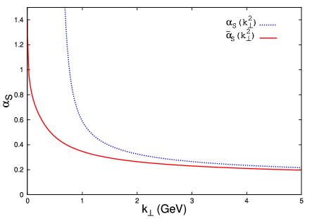
Figure 1: QCD couplings in NNLO. Dotted line (blue): standard coupling $\alpha_{S}(k_{\perp}^{2})$; continuous line (red): analytic time-like coupling $\tilde{\alpha}_{S}(k_{\perp}^{2})$.

Factorization and resummation of threshold logarithms in semileptonic decays leads to an expression for the the triple–differential distribution, the most general distribution, of the following form [19]:

$$\frac{1}{\Gamma}\frac{d^{3}\Gamma}{dxdwdu}\,=\,C[x,w;\alpha_{S}(Q)]\,\sigma[u;Q]\,+\,D[x,u,w;\alpha_{S}(Q)]\,,$$ (9)

where $x=\frac{2E_{l}}{m_{b}},~{}w=\frac{Q}{m_{b}},~{}u=\frac{1-\sqrt{1-(2m_{X}/Q)^{2}}}{1+\sqrt{1-(2m_{X}/Q)^{2}}}$ with $E_{l}$, $E_{X}$ and $m_{X}$ being the charged lepton energy, the total hadron energy and the hadron mass, respectively and the hard scale is given by $Q=2E_{X}$. $\Gamma=\Gamma(\alpha_{S})$ is the inclusive width of decay (1). Furthermore $C[x,w;\alpha_{S}]$ is a short–distance, process dependent hard factor and $D[x,u,w;\alpha_{S}]$ is a short–distance, process dependent, remainder function, vanishing in the threshold region $u\rightarrow 0$. The universal QCD form factor for heavy–to–light transitions, resumming to any order in $\alpha_{S}$ the series of logarithmically enhanced terms to some logarithmic accuracy, has the following exponential form in the Mellin moments $N$–space [20] $\!\!~{}^{,}$:

$$\log\sigma_{N}(Q)=\int_{0}^{1}\frac{dy}{y}[(1-y)^{N-1}\!-1]\Bigg{\{}\int_{Q^{2}y^{2}}^{Q^{2}y}\!\frac{dk_{\perp}^{2}}{k_{\perp}^{2}}\tilde{A}[\tilde{\alpha}_{S}(k_{\perp}^{2})]+\tilde{B}[\tilde{\alpha}_{S}(Q^{2}y)]+\tilde{D}[\tilde{\alpha}_{S}(Q^{2}y^{2})]\Bigg{\}}\,,$$ (10)

where the functions $A(\alpha_{S}),~{}B(\alpha_{S})$ and $D(\alpha_{S})$ have a standard fixed order expansions in ${\alpha}_{S}$. The prescription of our model is simply to replace the standard functions $A(\alpha_{S}),~{}B(\alpha_{S})$ and $D(\alpha_{S})$ with the functions $\tilde{A}(\tilde{\alpha}_{S}),~{}\tilde{B}(\tilde{\alpha}_{S})$ and $\tilde{D}(\tilde{\alpha}_{S})$ obtained from the standard ones by means of the change of renormalization scheme for the coupling constant $\alpha_{S}\rightarrow\tilde{\alpha}_{S}$.

Let us remark that even if our model doesn’t contain free parameters to be fitted to the data, in a certain sense we have “fitted” the model itself to data. In fact we have constructed our model among different possibilities (f.i. different possible prescriptions for the low energy behavior of the QCD coupling) (see f.i [8]). A further goal has been to describe at the best the very accurate data in $B$ fragmentation [5]. Then, by using the discussed perturbative analogy in the resummation formulas, we have made predictions for the spectra $B$ decays [1].

Threshold suppression — in our opinion the main theoretical ingredient for the measure of $|V_{ub}|$, as discussed in the introduction — is represented by the factor

$$W(a,b) \equiv \frac{\Gamma\left[B\rightarrow X_{u}\ell\nu_{\ell},p\in(a,b)\right]}{\Gamma\left[B\,\rightarrow\,X_{u}\,\ell\,\nu_{\ell}\right]}=\int_{a<p(x,w,u)<b}\frac{1}{\Gamma}\frac{d^{3}\Gamma}{dxdwdu}dxdwdu\,\leq\,1\,.$$ (11)

Note that:

$$W(p_{\min},p_{\max})\,=\,\int_{all}\frac{1}{\Gamma}\frac{d^{3}\Gamma}{dxdwdu}dxdwdu\,=\,1\,,$$ (12)

where by “all” we mean the whole phase–space of $x,\,w$ and $u$. For discussions and results on threshold resummed spectra of $B\rightarrow X_{u}\,\ell\,\nu_{\ell}$ decays at next–to–leading order see [9].

3 $|V_{ub}|$ extraction: method

The branching ratio in eq.(3) can be computed theoretically as:

$${\cal B}\left[p\in(a,b)\right]\!\! = \!\!\frac{\Gamma\left[B\rightarrow X_{u}\ell\,\nu_{\ell},~{}p\in(a,b)\right]}{\Gamma[B\rightarrow{\rm(anything)}]}=\tau_{B}\,\Gamma\big{[}B\,\rightarrow\,X_{u}\,\ell\,\nu_{\ell}\big{]}W(a,b).$$ (13)

Since we do not aim at checking QCD but only to extract $|V_{ub}|$, we can use the experimental measure of the $B$ lifetime, which is rather accurate:

$$\tau_{B}\,=\,(\,1.584\,\pm\,0.007\,)\times 10^{-12}\,{\rm s}\,,$$ (14)

and limit ourself to compute the suppression factor $W(a,b)$ defined in the previous section (see eq. (11)) and the inclusive $B\rightarrow X_{u}{\ell}\nu_{\ell}$ rate:

$$\Gamma\left[B\,\rightarrow\,X_{u}\,\ell\,\nu_{\ell}\right]\,=\,\frac{G_{F}^{2}\,m_{b}^{5}\,|V_{ub}|^{2}}{192\pi^{3}}\,F(\alpha_{S})\,.$$ (15)

QCD corrections are factorized in the function $F(\alpha_{S})$, which is of the form:

$$F(\alpha_{S})\,=\,1\,+\,\sum_{n=1}^{\infty}F_{n}\,\alpha_{S}^{n}\,,$$ (16)

with $F_{n}\sim\mathcal{O}(1)$ numerical coefficients. A measure of $|V_{ub}|$ is provided by direct comparison of eq. (13) with the corresponding experimental branching ratio. However, within this method, a large uncertainty comes from the dependence on the fifth power of the $b$–quark mass in eq. (15) .

One can eliminate the above (undesired) dependence on $m_{b}^{5}$, and the related uncertainty, by expressing the branching ratio as follows:

$${\cal B}\left[p\in(a,b)\right]\,=\,\frac{{\cal B}_{SL}}{1\,+\,{\cal R}_{c/u}}\,W(a,b)\,,$$ (17)

where we have defined the semileptonic branching ratio ($\ell$ is a fixed lepton species; in practice $\ell=e,\mu$):

$${\cal B}_{\rm SL}\,\equiv\,\frac{\Gamma(B\,\rightarrow\,X_{c}\,\ell\,\nu_{\ell})\,+\,\Gamma(B\,\rightarrow\,X_{u}\,\ell\,\nu_{\ell})}{\Gamma\left[B\,\rightarrow\,{\rm(anything)}\right]}$$ (18)

and the ratio of $(b\rightarrow c)/(b\rightarrow u)$ semileptonic widths:

$${\cal R}_{c/u}\,\equiv\,\frac{\Gamma(B\,\rightarrow\,X_{c}\,\ell\,\nu_{\ell})}{\Gamma(B\,\rightarrow\,X_{u}\,\ell\,\nu_{\ell})}\,.$$ (19)

Since ${\cal B}_{\rm SL}$ is rather well measured, one can give up on its theoretical calculation and replace it with the experimental determination [21]:

$${\cal B}_{\rm SL}\,=\,0.1066\,\pm\,0.0020\,.$$ (20)

As discussed in the introduction, $W(a,b)$ strongly depends on the modelling of the threshold region and is calculated according to the model whose main properties have been summarized in sec. 2, for the kinematical distributions listed in sec. 4.

This method presents no $m_{b}^{5}$ dependence, since one has to compute only the ratio of widths ${\cal R}_{c/u}$ and not the absolute widths. The semileptonic $b\rightarrow c$ width is conveniently written as:

$$\Gamma(B\,\rightarrow\,X_{c}\,\ell\,\nu_{\ell})\,=\,\frac{G_{F}^{2}\,m_{b}^{5}\,|V_{cb}|^{2}}{192\pi^{3}}\,I(\rho)\,F(\alpha_{S})\,G(\alpha_{S},\rho)\,,$$ (21)

where

$$\rho\,\equiv\,\frac{m_{c}^{2}}{m_{b}^{2}}\,\approx 0.1\,.$$ (22)

The function $I(\rho)$ accounts for the suppression of phase–space because of $m_{c}\neq 0$ [22] :

$$I(\rho)\,=\,1-8\rho+12\rho^{2}\log\frac{1}{\rho}+8\rho^{3}-\rho^{4}\,.$$ (23)

Note that there is an (accidental) strong dependence on the charm mass $m_{c}$, because of the appearance of a large factor in the leading term in $\rho$, namely $-\,8$. As far as inclusive quantities are concerned, the largest source of theoretical error comes indeed from the uncertainty in $\rho$. Most of the dependence is actually on the difference $m_{b}-m_{c}$, which can be estimated quite reasonably within the Heavy Quark Effective Theory (HQET) — see next section. Finally, the factor $G(\alpha_{S},\rho)$ contains corrections suppressed by powers of $\alpha_{S}$ as well by powers of $\rho$:

$$G(\alpha_{S},\rho)\,=\,1\,+\,\sum_{n=1}^{\infty}G_{n}(\rho)\,\alpha_{S}^{n}\,,$$ (24)

with $G_{n}(0)=0$. Note that $G(0,\rho)=G(\alpha_{S},0)=1\,$. By inserting the above expressions for the semileptonic rates, one obtains for the perturbative expansion of ${\cal R}_{c/u}$:

$${\cal R}_{c/u}\,=\,{\cal R}_{c/u}\left(\rho,\alpha_{S},|V_{ub}|/|V_{cb}|\right)\,=\,\frac{|V_{cb}|^{2}}{|V_{ub}|^{2}}\,I(\rho)\,G(\alpha_{S},\rho)\,.$$ (25)

Let us stress that this method actually provides a measure of the ratio $|V_{ub}|/|V_{cb}|$, but since the error on $|V_{cb}|$ is rather small and theoretically well understood, one is basically measuring $|V_{ub}|$.

We prefer to use the method based on the computation of the ratio of $(b\rightarrow c)/(b\rightarrow u)$ semileptonic rates ${\cal R}_{c/u}$ (see eq. (19)), instead of the method involving the absolute $b\,\rightarrow\,u\,\ell\,\nu_{\ell}$ rate (see eq. (15)), because in the former case only ratios of inclusive widths need to be evaluated. As a consequence, while eq. (15) depends on the absolute value of $m_{b}$, eq. (19) depends mostly on the difference $m_{b}$ $-$$m_{c}$, opening the possibility of partial cancellation of hadronic uncertainties. However, the two methods give compatible values of $|V_{ub}|$ and the method based on eq. (15) is used to estimate the systematic error on the method based on eq. (19). The fact that the two methods give similar results corroborates the conclusion that differences with respect to previous analyses originate from a smaller suppression in the threshold region in our model compared to previous models, rather than from different estimates of inclusive quantities, i.e. different choices of quark masses, QCD coupling, etc. In other words, we do not obtain a small value of $|V_{ub}|$ by an ad–hoc choice of quark masses $m_{b}$ and $m_{c}$ or of $\alpha_{S}(m_{Z})$. The difference lies in the different modelling of the threshold region.

3.1 Quark masses

Since quarks are confined inside observable hadrons, their masses cannot be directly measured and their values are biased by the selected theoretical framework. It is well known that pole masses are affected by the poor behavior of the perturbative series relating them to physical quantities; replacing the pole mass with the $\overline{\mbox{MS}}$ mass in dimensional regularization slightly improves the asymptotic behavior of the series. Several alternative definitions of the $b$–quark mass have been introduced in the literature [23], in order to give a better convergence of the first (few) orders of the perturbative series and consequently reduce the theoretical errors.

We have performed the calculation in the $\overline{\mbox{MS}}$ mass scheme. The $\overline{\mbox{MS}}$ masses for the $b$ and the $c$ quark are taken $\overline{m}_{b}(\overline{m}_{b})=4.20\,\pm 0.07\,\rm{GeV}$ and $\overline{m}_{c}(\overline{m}_{c})=1.25\,\pm 0.09\,\rm{GeV}$ [21], respectively. However, in order to take into account the uncertainties coming from a different scheme definition, we have considered the pole–mass scheme as well. The HQET in lowest order (static theory) gives the following relation for the difference of the on–shell beauty and charm mass:

$$m_{b}\,-\,m_{c}\,=\,m_{B}\,-\,m_{D}\,+\,\mathcal{O}\left[\mathchar 28931\relax^{2}\left(\frac{1}{m_{c}}-\frac{1}{m_{b}}\right)\right]$$ (26)

with

$$m_{B}\,-\,m_{D}\,\simeq\,3.41~{}\mathrm{\,Ge\kern-1.00006ptV}\,.$$ (27)

This value is also consistent with the mass estimates in the $\rm{kin_{EXP}}$ and $1\,S_{\rm{EXP}}$ schemes [24]. The leading corrections to (26), $\mathcal{O}[\mathchar 28931\relax^{2}(1/m_{c}-1/m_{b})]$, involve the chromomagnetic operator and the kinetic one. One can cancel the chromomagnetic corrections by taking the “spin–averaged” meson masses [25]:

$$m_{b}\,-\,m_{c}\simeq\frac{m_{B}+3\,m_{B^{\star 0}}}{4}\,-\,\frac{m_{D}+3\,m_{D^{\star 0}}}{4}\,+\,\cdots\,,$$ (28)

where the smaller difference of $\approx 70$ MeV, implies, for a fixed beauty mass, a heavier charm quark mass:

$$\frac{m_{B}+3\,m_{B^{\star 0}}}{4}\,-\,\frac{m_{D}+3\,m_{D^{\star 0}}}{4}\,\simeq\,3.34~{}\mathrm{\,Ge\kern-1.00006ptV}\,.$$ (29)

For a consistent subleading computation one also needs the kinetic contribution, which cannot be extracted from the data and it is computed theoretically [24, 26]. The conclusion is that we consider safe to eliminate the $c$ pole charm mass by using a range of $m_{b}-m_{c}$ given by eqs. (26) and (28).

4 Results

This is the central section of the paper in which we determine $|V_{ub}|$ from measured semileptonic branching fractions, in limited regions of the phase–space, and we perform the corresponding averages. The experimental analyses are categorized according to the kinematical distribution looked at, where selection criteria are applied to define the limited phase–space on which the branching ratio is computed. The analyses are:

1. $E_{\ell}$: where the distribution looked at is the lepton energy ($E_{\ell}$). There are results from BABAR [28], Belle [29] and CLEO [30]. The lepton energy ranges from 1.9, 2.0 and 2.1 $\mathrm{\,Ge\kern-1.00006ptV}$ for Belle, BABAR, and CLEO, respectively, up to 2.6 $\mathrm{\,Ge\kern-1.00006ptV}$. As described in ref. [1], we will look only at the range where data are not affected by potential $b\rightarrow c\,\ell\,\nu_{\ell}$ background: 2.3 $\mathrm{\,Ge\kern-1.00006ptV}$ $<$ $E_{\ell}$ $<$ 2.6 $\mathrm{\,Ge\kern-1.00006ptV}$.

2. $m_{X}$: where the distribution looked at is the invariant mass of the hadron final state ($m_{X}$). Both BABAR [31] and Belle [32] have performed one analysis for $m_{X}$ $<$ 1.55 $\mathrm{\,Ge\kern-1.00006ptV}$ and $m_{X}$ $<$ 1.7 $\mathrm{\,Ge\kern-1.00006ptV}$, respectively. The selection strategy is based on the full reconstruction of the $B$ meson on the other side of the event ($B$–reconstruction analysis). The same selected events are looked at also by using two other kinematical distributions: $(m_{X},q^{2})$ and $P_{+}$, as we will see below. In all the three cases a lower cut on the photon energy at 1 $\mathrm{\,Ge\kern-1.00006ptV}$ is applied.

3. $P_{+}$: where the distribution looked at is $P_{+}\equiv E_{X}-|\vec{p}_{X}|$, $E_{X}$ and $\vec{p}_{X}$ being the energy and the magnitude of the 3–momentum of the hadronic system, respectively. The $B$–reconstruction analysis is used. There are both BABAR [31] and Belle [32] results. Both analyses require $P_{+}<$ 0.66 $\mathrm{\,Ge\kern-1.00006ptV}$.

4. $(m_{X},q^{2})$: where the distribution looked at is a two dimensional distribution in the plane of the hadronic mass and the transferred squared momentum $q^{2}$ to the lepton pair. The analyses from BABAR and Belle are described in [31] and [32], respectively, using the $B$–reconstruction analysis. Moreover, another technique, called simulated annealing, is used by Belle to select events in the $(m_{X},q^{2})$ plane [33]. Events with hadron mass lower than 1.7 $\mathrm{\,Ge\kern-1.00006ptV}$ and $q^{2}$ larger than 8 $\mathrm{\,Ge\kern-1.00006ptV}^{2}$ are selected in all the cases.

5. $(E_{\ell},s_{\mathrm{h}}^{\mathrm{max}})$: where the distribution looked at is a two dimensional distribution in the electron energy and $s_{\mathrm{h}}^{\mathrm{max}}$, the maximal $m_{X}^{2}$ at fixed $q^{2}$ and $E_{\ell}$. There is a result from BABAR [34]. The requests on the kinematic variables are $E_{\ell}$ $>2.0\mathrm{\,Ge\kern-1.00006ptV}$ and $s_{\mathrm{h}}^{\mathrm{max}}\ <3.5\mathrm{\,Ge\kern-1.00006ptV}^{2}$.

We compute $|V_{ub}|$ for each of the analyses starting from the corresponding partial branching fractions. Then, we determine the average $|V_{ub}|$ value using the HFAG methodology [10], together with Ref.[35].

Table 1 reports the extracted values of $|V_{ub}|$ for all the analysis methods and their corresponding average. The errors are experimental (i.e. statistical and systematic) and theoretical, respectively. The average is:

$$|V_{ub}|\,=\,(\,3.76\,\pm\,0.13\,\pm\,0.22\,)\times 10^{-3}\,,$$ (30)

consistent with the measured value of $|V_{ub}|$ from exclusive decays [10] and the indirect measure [11]. The correlation among the analyses has been taken into account when performing the average .

The table shows also the criteria used for the determination of the partial branching ratio ($\Delta{\cal B}$). The $|V_{ub}|$ values and the corresponding average are plotted in Figure 2.

Table 1: The first column in the table shows the analyses used in the average, the second column shows the corresponding values of $|V_{ub}|$, and finally the last column shows the criteria for which $\Delta{\cal B}$ is available. The final row shows the average value of $|V_{ub}|$. The errors on the $|V_{ub}|$ values are experimental and theoretical, respectively. The experimental error includes both the statistical and systematic errors.

Analysis	$|V_{ub}|$ ($10^{-3}$)	$\Delta{\cal B}$ criteria
BABAR ($E_{\ell}$) [28]	3.46$\pm$ 0.14 ${}^{+0.23}_{-0.23}$	$E_{\ell}$ $>2.3$$\mathrm{\,Ge\kern-1.00006ptV}$
Belle ($E_{\ell}$) [29]	3.25$\pm$ 0.17 ${}^{+0.22}_{-0.21}$	$E_{\ell}$ $>2.3$$\mathrm{\,Ge\kern-1.00006ptV}$
CLEO ($E_{\ell}$) [30]	3.49$\pm$ 0.20 ${}^{+0.23}_{-0.23}$	$E_{\ell}$ $>2.3$$\mathrm{\,Ge\kern-1.00006ptV}$
BABAR ($m_{X}$) [31]	4.04$\pm$ 0.19 ${}^{+0.24}_{-0.24}$	$m_{X}$ $<1.55$ $\mathrm{\,Ge\kern-1.00006ptV}$
Belle ($m_{X}$) [32]	3.93$\pm$ 0.26 ${}^{+0.23}_{-0.23}$	$m_{X}$ $<1.7$ $\mathrm{\,Ge\kern-1.00006ptV}$
BABAR ($(m_{X},q^{2})$) [31]	4.14$\pm$ 0.26 ${}^{+0.23}_{-0.23}$	$m_{X}$ $<1.7$ $\mathrm{\,Ge\kern-1.00006ptV}$, $q^{2}>8$ $\mathrm{\,Ge\kern-1.00006ptV}^{2}$
Belle $(m_{X},q^{2})$ [33]	3.95$\pm$ 0.42 ${}^{+0.22}_{-0.22}$	$m_{X}$ $<1.7$ $\mathrm{\,Ge\kern-1.00006ptV}$, $q^{2}>8$ $\mathrm{\,Ge\kern-1.00006ptV}^{2}$
BABAR $(E_{\ell},s_{\mathrm{h}}^{\mathrm{max}})$[34]	3.87$\pm$ 0.26 ${}^{+0.23}_{-0.24}$	$E_{\ell}$ $>2.0$ $\mathrm{\,Ge\kern-1.00006ptV}$, $s_{\mathrm{h}}^{\mathrm{max}}$$<3.5$ $\mathrm{\,Ge\kern-1.00006ptV}^{2}$
BABAR ($P_{+}$) [31]	3.45$\pm$ 0.22 ${}^{+0.21}_{-0.37}$	$P_{+}$ $<0.66$ $\mathrm{\,Ge\kern-1.00006ptV}$
Average	3.76$\pm$ 0.13 ${}^{+0.22}_{-0.22}$

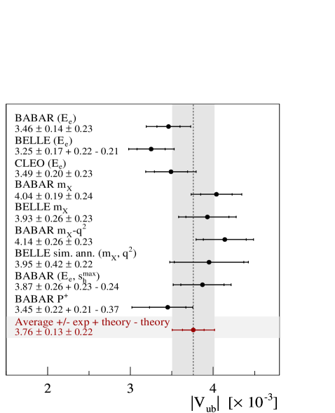
Figure 2: $|V_{ub}|$ values for the analyses used in the average and their average.

Several sources of theoretical errors have been considered:

• in addition to our preferred method based on eq. (17), we also use the method based on eq. (15) to extract the value of $|V_{ub}|$. Since the two methods described in the previous section basically involve different inclusive quantities, this error allows a cross–check of their evaluations, i.e. basically of the choices of the $b$ and $c$ masses adopted;

• we compute inclusive quantities both in the $\overline{\mbox{MS}}$ and pole schemes for the quark masses. The $|V_{ub}|$ value using the $\overline{\mbox{MS}}$ masses is our default, the value using the pole scheme masses, where the ranges defined in sec. 3.1 are used, gives the systematic uncertainty. Since in general higher–order corrections are different in the two schemes, that should provide an estimate of the size of unknown higher–order effects.

• we vary the order at which the rate is computed from the exact NLO to the approximate NNLO [36]. Since the perturbative series for QCD is believed to be an asymptotic one and $\alpha_{S}=\alpha_{S}(m_{b})\approx 0.22$ in $b$ physics is rather large, that should provide a reasonable estimate on the truncation error;

• we vary all the parameters which enter in the computation of $|V_{ub}|$ within their errors, as given by the PDG [21].

What we cannot change is the modelling of the threshold region represented by the factor $W(a,b)$, which is fixed in our model, as discussed in the introduction. How good it such modelling of the threshold region can only be estimated indirectly, by considering different decay spectra, where presumably threshold effects enter in different ways.

Future work towards improving the determination of the $b$–quark mass in the $\overline{\mbox{MS}}$ and the pole scheme will help in reducing our error on $|V_{ub}|$.

Table 2 reports the fractional contributions to the theoretical errors due to the different sources. A large excursion of the error among the analyses is due to $\alpha_{S}$, which varies from a minimum of $\pm 0.6\%$ for the $(m_{X},q^{2})$  analyses to a maximum of $\pm 3.5\%$ for the endpoint analyses. The largest contributions to the error are given by the charm mass in the $\overline{\mbox{MS}}$ scheme ($\pm 4.4\%$) and the variation from the $\overline{\mbox{MS}}$ to the pole scheme (from $-\,1.3\%$ to $-\,5.2\%$ starting from lower to higher masses), due to the conservatively larger error used for the pole scheme mass.

Table 3 shows the $|V_{ub}|$ averages for different analysis categories. Note that the $(m_{X},q^{2})$ analyses tend to have the largest values of $|V_{ub}|$, while the endpoint analyses the smallest.

Table 2: The first column of the table shows the different contributions to the theoretical errors, the second column shows the corresponding variation, and finally the third column shows the percentage contribution with respect to the $|V_{ub}|$ value.

Theoretical Errors
Contribution	Variation	Error (%)
$\alpha_{S}$	$0.1176\pm 0.0024$	$\pm 0.6\rightarrow 3.5$
$|V_{cb}|$	$(41.6\pm 0.6)\times 10^{-3}$	$\pm 1.4$
$m_{b}$ ($\mathrm{\,Ge\kern-1.00006ptV}$)	$4.20\pm 0.07$	$\pm 0.6$
$m_{c}$ ($\mathrm{\,Ge\kern-1.00006ptV}$)	$1.25\pm 0.09$	$\pm 4.4$
${\cal B}$ ($B\rightarrow X_{u}{\ell}\nu_{\ell}$)	$0.1066\pm 0.0020$	$\pm 1.0$
$|V_{ub}|$ method		$+0.8$
pole mass ($\mathrm{\,Ge\kern-1.00006ptV}$)	$\begin{array}[]{c}4.7<m_{b}<5.0,\,\,1.47<m_{c}<1.83\\ 3.34<m_{b}-m_{c}<3.41\end{array}$	$-1.3\rightarrow-5.2$
approx. NNLO rate		$+2.0$

Table 3: The table contains the $|V_{ub}|$ values for several analyses and the corresponding averages. The errors on the $|V_{ub}|$ values are experimental and theoretical, respectively. The experimental error includes both the statistical and systematic errors.

$|V_{ub}|$ for endpoint analyses ($10^{-3}$)
BABAR ($E_{\ell}$) [28]	3.46$\pm$ 0.14 ${}^{+0.23}_{-0.23}$	$E_{\ell}$ $>2.3$ $\mathrm{\,Ge\kern-1.00006ptV}$
Belle ($E_{\ell}$) [29]	3.25$\pm$ 0.17 ${}^{+0.22}_{-0.21}$	$E_{\ell}$ $>2.3$ $\mathrm{\,Ge\kern-1.00006ptV}$
CLEO ($E_{\ell}$) [30]	3.49$\pm$ 0.20 ${}^{+0.23}_{-0.23}$	$E_{\ell}$ $>2.3$ $\mathrm{\,Ge\kern-1.00006ptV}$
Average	3.43$\pm$ 0.15 ${}^{+0.23}_{-0.22}$
$|V_{ub}|$ for $m_{X}$ analyses ($10^{-3}$)
BABAR ($m_{X}$) [31]	4.04$\pm$ 0.19 ${}^{+0.24}_{-0.24}$	$m_{X}$ $<1.55$ $\mathrm{\,Ge\kern-1.00006ptV}$
Belle ($m_{X}$) [32]	3.93$\pm$ 0.26 ${}^{+0.23}_{-0.22}$	$m_{X}$ $<1.7$ $\mathrm{\,Ge\kern-1.00006ptV}$
Average	4.00$\pm$ 0.16 ${}^{+0.24}_{-0.23}$
$|V_{ub}|$ for $(m_{X},q^{2})$  analyses ($10^{-3}$)
BABAR $(m_{X},q^{2})$ [31]	4.14$\pm$ 0.26 ${}^{+0.23}_{-0.23}$	$m_{X}$ $<1.7$ $\mathrm{\,Ge\kern-1.00006ptV}$, $q^{2}>8~{}\mathrm{\,Ge\kern-1.00006ptV}^{2}$
Belle $(m_{X},q^{2})$ [32]	4.21$\pm$ 0.37 ${}^{+0.23}_{-0.23}$	$m_{X}$ $<1.7$ $\mathrm{\,Ge\kern-1.00006ptV}$, $q^{2}>8~{}\mathrm{\,Ge\kern-1.00006ptV}^{2}$
Belle $(m_{X},q^{2})$ [33]	3.95$\pm$ 0.42 ${}^{+0.22}_{-0.22}$	$m_{X}$ $<1.7$ $\mathrm{\,Ge\kern-1.00006ptV}$, $q^{2}>8~{}\mathrm{\,Ge\kern-1.00006ptV}^{2}$
Average	4.13$\pm$ 0.21 ${}^{+0.23}_{-0.23}$
$|V_{ub}|$ for $P_{+}$  analyses ($10^{-3}$)
BABAR ($P_{+}$) [31]	3.45$\pm$ 0.22 ${}^{+0.21}_{-0.37}$	$P^{+}<0.66$
Belle ($P_{+}$) [32]	3.73$\pm$ 0.32 ${}^{+0.23}_{-0.29}$	$P^{+}<0.66$
Average	3.55$\pm$ 0.19 ${}^{+0.21}_{-0.23}$

The larger value of $|V_{ub}|$ coming from the analysis of the double distribution in $(m_{X},q^{2})$ is expected on qualitative basis. For $m_{X}=0$, the hard scale $Q$ is given by

$$Q\,=\,m_{B}\,-\,\frac{q^{2}}{m_{B}}\,<\,0.71\,m_{B}\,,$$ (31)

because $q^{2}\,>\,8~{}\mathrm{\,Ge\kern-1.00006ptV}^{2}$. The lower cut on $q^{2}$ therefore significantly reduces the hard scale $Q$ from the “natural” value $Q=m_{B}$. The point is that our model has been constructed to describe $B$–decay spectra having the (maximal) hard scale $Q=m_{B}$, and not spectra having a smaller hard scale. Indeed, the model was checked against beauty fragmentation at the $Z^{0}$ peak [5], where the dominant infrared effects are controlled by a hard scale equal to $m_{B}$. In other words, to analyze the $(m_{X},q^{2})$ distribution, we are using the model in a region where it has not been checked and it is no surprise that it does not work so well in this case.

5 Conclusions

We have analyzed semileptonic $B$ decay data in the framework of a model for QCD non–perturbative effects based on an effective time-like QCD coupling, free from Landau singularities. The analysis has considered the kinematical distributions in $E_{\ell}$, $m_{X}$, and $P_{+}$, as well as the two dimensional distributions in $(m_{X},q^{2})$ and $(E_{\ell},s_{\mathrm{h}}^{\mathrm{max}})$, taking into account the experimental kinematical cuts.

Our inclusive measure of the $|V_{ub}|$ CKM matrix element is:

$$|V_{ub}|\,=\,(\,3.76\,\pm\,0.13\,\pm\,0.22\,)\times 10^{-3}\,.$$ (32)

The errors on the $|V_{ub}|$ value are experimental and theoretical, respectively. The experimental error includes both the statistical and systematic errors.

For the first time, an inclusive value for $|V_{ub}|$ is obtained which is in complete agreement with the exclusive determination. Current literature presents a discrepancy among previous inclusive determinations of $|V_{ub}|$ on one side and the exclusive determinations ($\approx 2\,\sigma$) and the over–all fit of the Standard Model ($\approx 3\,\sigma$) on the other side[10].

Let us try to identify the differences between our approach and the previous ones. A first difference lies in the selected lepton energy range. According to our analysis, lepton spectra below $\approx 2.3$ $\mathrm{\,Ge\kern-1.00006ptV}$ measured at the $B$–factories suffer from an under–subtracted charm background. Because of that, we have limited our analysis to pretty large lepton energies $E_{\ell}>2.3$ $\mathrm{\,Ge\kern-1.00006ptV}$. If we take a smaller cutoff, we obtain up to a $\approx+2.7\%$ larger average value of $|V_{ub}|$, in order to simulate $b\rightarrow c$ events. As far as theory is concerned, our model seems to produce a smaller Sudakov suppression compared to other models constructed on top of soft–gluon resummation, such as for example the dressed gluon exponentiation [16]. For a fixed experimental rate, a smaller Sudakov suppression implies indeed larger hadronic form factors and smaller $|V_{ub}|$’s. As discussed above, our confidence in the model is also based on phenomenological grounds; we have checked it in beauty fragmentation [5], where soft contributions are similar to those in $b$ decay.

In conclusion, the inclusive extraction of $|V_{ub}|$ requires the calculation of inclusive quantities, strongly dependent on $b$ and $c$ masses, as well as the evaluation of threshold–suppressed quantities, the latter containing large infrared logarithms and Fermi–motion (non–perturbative) effects. We argue that the main difference of our model with respect to previous ones is a smaller suppression of the threshold region.

Acknowledgments

This work is supported in part by the EU Contract No. MRTN-CT-2006-035482 “FLAVIAnet”.

References

- [1] U. Aglietti, G. Ferrera and G. Ricciardi, Nucl. Phys. B 768 (2007) 85 [arXiv:hep-ph/0608047].
- [2] N. Cabibbo, Phys. Rev. Lett. 10, 531 (1963); M. Kobayashi and T. Maskawa, Prog. Theor. Phys. 49, 652 (1973).
- [3] For a recent reviw see for example: B. Grinstein, In the Proceedings of 5th Flavor Physics and CP Violation Conference (FPCP 2007), Bled, Slovenia, 12-16 May 2007, pp 005 [arXiv:0706.4173 [hep-ph]].
- [4] D. V. Shirkov and I. L. Solovtsov, Phys. Rev. Lett. 79 (1997) 1209 [arXiv:hep-ph/9704333].
- [5] U. Aglietti, G. Corcella and G. Ferrera, Nucl. Phys. B 775 (2007) 162 [arXiv:hep-ph/0610035].
- [6] G. Altarelli, N. Cabibbo, G. Corbò, L. Maiani and G. Martinelli, Nucl. Phys. B 208 (1982) 365.
- [7] S. Catani, M. L. Mangano, P. Nason and L. Trentadue, Phys. Lett. B 378 (1996) 329 [arXiv:hep-ph/9602208].
- [8] U. Aglietti and G. Ricciardi, Phys. Rev. D 70 (2004) 114008 [arXiv:hep-ph/0407225].
- [9] U. Aglietti, G. Ricciardi and G. Ferrera, Phys. Rev. D 74 (2006) 034004 [arXiv:hep-ph/0507285]; Phys. Rev. D 74 (2006) 034005 [arXiv:hep-ph/0509095]; Phys. Rev. D 74 (2006) 034006 [arXiv:hep-ph/0509271].
- [10] E. Barberio et al., arXiv:0808.1297 [hep-ex]. and online HFAG updates for ICHEP08.
- [11] M. Bona et al. [UTfit Collaboration], JHEP 0610 (2006) 081 [arXiv:hep-ph/0606167].
- [12] M. Bona et al. [UTfit Collaboration], JHEP 0603 (2006) 080 [arXiv:hep-ph/0509219]; G. Isidori and P. Paradisi, Phys. Lett. B 639 (2006) 499 [arXiv:hep-ph/0605012]; W. Altmannshofer, A. J. Buras, D. Guadagnoli and M. Wick, arXiv:0706.3845 [hep-ph].
- [13] A. K. Leibovich, I. Low and I. Z. Rothstein, Phys. Rev. D 61 (2000) 053006 [arXiv:hep-ph/9909404]; R. Akhoury and I. Z. Rothstein, Phys. Rev. D 54 (1996) 2349 [arXiv:hep-ph/9512303]; A. K. Leibovich, I. Low and I. Z. Rothstein, Phys. Lett. B 486 (2000) 86 [arXiv:hep-ph/0005124].
- [14] M. Neubert, Phys. Lett. B 513 (2001) 88 [arXiv:hep-ph/0104280]; B. O. Lange, M. Neubert and G. Paz, JHEP 0510 (2005) 084 [arXiv:hep-ph/0508178];
- [15] C. W. Bauer, Z. Ligeti and M. E. Luke, Phys. Rev. D 64 (2001) 113004 [arXiv:hep-ph/0107074].
- [16] E. Gardi, JHEP 0404 (2004) 049 [arXiv:hep-ph/0403249]; J. R. Andersen and E. Gardi, JHEP 0601 (2006) 097 [arXiv:hep-ph/0509360].
- [17] S. W. Bosch, B. O. Lange, M. Neubert and G. Paz, Nucl. Phys. B 699 (2004) 335 [arXiv:hep-ph/0402094]; B. O. Lange, M. Neubert and G. Paz, Phys. Rev. D 72 (2005) 073006 [arXiv:hep-ph/0504071].
- [18] P. Gambino, P. Giordano, G. Ossola and N. Uraltsev, JHEP 0710 (2007) 058 [arXiv:0707.2493 [hep-ph]].
- [19] U. Aglietti, Nucl. Phys. B 610 (2001) 293 [arXiv:hep-ph/0104020].
- [20] S. Catani and L. Trentadue, Nucl. Phys. B 327 (1989) 323; G. Sterman, Nucl. Phys. B 281 (1987) 310.
- [21] C. Amsler et al. [Particle Data Group], Phys. Lett. B 667 (2008) 1.
- [22] Y. Nir, Phys. Lett. B 221, 184 (1989).
- [23] see, f.i.: I. I. Y. Bigi, M. A. Shifman, N. Uraltsev and A. I. Vainshtein, Phys. Rev. D 56 (1997) 4017 [arXiv:hep-ph/9704245]; I. I. Y. Bigi, M. A. Shifman, N. Uraltsev and A. I. Vainshtein, Phys. Rev. D 56 (1997) 4017 [arXiv:hep-ph/9704245]; A. H. Hoang and T. Teubner, Phys. Rev. D 60 (1999) 114027 [arXiv:hep-ph/9904468]; M. Beneke, Phys. Rev. D 434 (1998) 115; A. H. Hoang, Z. Ligeti, and A. V. Manohar, Phys. Rev. Lett. 82 (1999) 277.
- [24] C.W. Bauer, Z. Ligeti, M. Luke, A. Manohar, M. Trott, Phys. Rev. D 70 (2004) 094017 [arXiv:hep-ph/0408002v3].
- [25] U. Aglietti, Phys. Lett. B 281 (1992) 341.
- [26] A. H. Hoang and A. V. Manohar, Phys. Lett. B 633 (2006) 526 [arXiv:hep-ph/0509195]; O. Buchmuller and H. Flacher, Phys. Rev. D 73 (2006) 073008 [arXiv:hep-ph/0507253].
- [27] A. Czarnecki, M. Jezabek and J. H. Kuhn, Phys. Lett. B 346 (1995) 335 [arXiv:hep-ph/9411282].
- [28] B. Aubert et al. [BABAR Collaboration], Phys. Rev. D 73, 012006 (2006) [arXiv:hep-ex/0509040].
- [29] A. Limosani et al. [Belle Collaboration], Phys. Lett. B 621 (2005) 28 [arXiv:hep-ex/0504046].
- [30] A. Bornheim et al. [CLEO Collaboration], Phys. Rev. Lett. 88 (2002) 231803 [arXiv:hep-ex/0202019].
- [31] B. Aubert et al. [BABAR Collaboration], arXiv:0708.3702 [hep-ex], accepted by PRL.
- [32] I. Bizjak et al. [Belle Collaboration], Phys. Rev. Lett. 95 (2005) 241801 [arXiv:hep-ex/0505088].
- [33] H. Kakuno et al. [Belle Collaboration], Phys. Rev. Lett. 92 (2004) 101801 [arXiv:hep-ex/0311048].
- [34] B. Aubert et al. [BABAR Collaboration], Phys. Rev. Lett. 95 (2005) 111801, Erratum-ibid. 97 (2006) 019903 [arXiv:hep-ex/0506036].
- [35] R. Barlow, IPPP/02/39 [arXiv:hep-ex/0207026].
- [36] T. van Ritbergen, Phys. Lett. B 454 (1999) 353 [arXiv:hep-ph/9903226]; A. Czarnecki and K. Melnikov, Phys. Rev. D 59 (1999) 014036 [arXiv:hep-ph/9804215].
- [37] I. I. Y. Bigi, M. A. Shifman, N. G. Uraltsev and A. I. Vainshtein, Int. J. Mod. Phys. A 9 (1994) 2467 [arXiv:hep-ph/9312359].