$D^{0}$ Mixing at Belle

Abstract

We report the recent two results of $D^{0}$-$\overline{D}{}^{\,0}$ mixing studies at Belle in $D^{0}\to K^{+}K^{-}/\pi^{+}\pi^{-}$ and $D^{0}\to K_{S}^{0}\pi^{+}\pi^{-}$ decays. The former measures the relative difference of the lifetimes $y_{CP}$, giving the evidence of $D^{0}$-$\overline{D}{}^{\,0}$ mixing; the latter measures the $D^{0}$ mixing parameters $x$ and $y$.

I Introduction

Mixing phenomenon, i.e. the oscillation of a neutral meson into its corresponding anti-meson as a function of time, has been observed in the $K^{0}$, $B^{0}$, and most recently $B^{0}_{s}$ systems. This process is also possible in the $D$-meson system, but has not previously been observed.

Mixing in heavy flavor systems such as that of $B^{0}$ and $B_{s}^{0}$ is governed by the short-distance box diagram. However, in the $D^{0}$ system this diagram is both GIM-suppressed and doubly-Cabibbo-suppressed relative to the amplitude dominating the decay width, and thus the short-distance rate is very small. Consequently, $D^{0}$-$\overline{D}{}^{\,0}$ mixing is expected to be dominated by long-distance processes that are difficult to calculate; theoretical estimates for the mixing parameters $x=(m_{1}-m_{2})/\Gamma$ and $y=(\Gamma_{1}-\Gamma_{2})/2\Gamma$ range over two-three orders of magnitude Petrov . Here, $m_{1},m_{2}$ ($\Gamma_{1},\Gamma_{2}$) are the masses (decay widths) of the mass eigenstates $|D_{1,2}\rangle=p|D^{0}\rangle\pm q|\overline{D}{}^{\,0}\rangle$, and $\Gamma=(\Gamma_{1}+\Gamma_{2})/2$. The parameters $p$ and $q$ are complex coefficients satisfying $|p|^{2}+|q|^{2}=1$.

The general experimental method identifies the flavor of the neutral $D$ meson when produced by reconstructing the decay $D^{*+}\to D^{0}\pi^{+}$ or $D^{*-}\to\overline{D}{}^{\,0}\pi^{-}$ charge_conjugates ; the charge of the accompanying pion identifies the $D$ flavor. Because the energy release in $D^{*}$ decays is only $\sim 6$ MeV, the background is largely suppressed. The $D^{0}$ decay time ($t$) is calculated via $(l/p)\times m_{D^{0}}$, where $l$ is the distance between the $D^{*}$ and $D^{0}$ decay vertices and $p$ is the $D^{0}$ momentum. The $D^{*}$ vertex position is taken to be the intersection of the $D^{0}$ momentum with the beamspot profile. To reject $D^{(*)}$ decays originating from $B$ decays, one requires $p_{D^{*}}>2.5$ GeV, which is the kinematic endpoint.

II $CP$-eigenstates $K^{+}K^{-}$ and $\pi^{+}\pi^{-}$

We have studied the decays to $CP$ eigenstates $D^{0}\!\rightarrow\!K^{+}K^{-}$and $D^{0}\!\rightarrow\!\pi^{+}\pi^{-}$; treating the decay-time distributions as exponential, we measured the quantity

$$y_{CP}=\frac{\tau_{K^{-}\pi^{+}}}{\tau_{K^{+}K^{-}}}-1,$$ (1)

where $\tau_{K^{-}\pi^{+}}$ and $\tau_{K^{+}K^{-}}$ are the lifetimes of $D^{0}\to K^{-}\pi^{+}$ and $D^{0}\!\rightarrow\!K^{+}K^{-}$(or $D^{0}\!\rightarrow\!\pi^{+}\pi^{-}$) decays. It can be shown that $y_{CP}=y\cos\phi-\frac{1}{2}A_{M}x\sin\phi$ ycpeqn , where $A_{M}$ parameterizes $CPV$ in mixing and $\phi$ is a weak phase. If $CP$ is conserved, $A_{M}=\phi=0$ and $y_{CP}=y$. This method has been used by numerous experiments to constrain $y_{\rm CP}$ ycp_references . Our measurement, based on 540 fb^-1 data, yields a nonzero value of $y_{CP}$ with $>3\sigma$ significance belle_kk . We also searched for $CPV$ by measuring the quantity

$$A_{\Gamma}=\frac{\tau(\overline{D}{}^{\,0}\to K^{-}K^{+})-\tau(D^{0}\to K^{+}K^{-})}{\tau(\overline{D}{}^{\,0}\to K^{-}K^{+})+\tau(D^{0}\!\rightarrow\!K^{+}K^{-})};$$ (2)

this observable equals $A_{\Gamma}=\frac{1}{2}A_{M}y\cos\phi-x\sin\phi$ ycpeqn .

We reconstruct $D^{*+}\to D^{0}\pi_{s}^{+}$ decays and $D^{0}\!\rightarrow\!K^{+}K^{-}$, $K^{-}\pi^{+}$, and $\pi^{+}\pi^{-}$. Candidate $D^{0}$ mesons are selected using two kinematic observables: the invariant mass of the $D^{0}$ decay products, $M$, and the energy release in the $D^{*+}$ decay, $Q=(M_{D^{*}}-M-m_{\pi^{+}})c^{2}$. According to Monte Carlo (MC) simulated distributions of $t$, $M$ and $Q$, background events fall into four categories: (1) combinatorial, with zero apparent lifetime; (2) true $D^{0}$ mesons combined with random slow pions (this has the same apparent lifetime as the signal) (3) $D^{0}$ decays to three or more particles, and (4) other charm hadron decays. The apparent lifetime of the latter two categories is 10-30% larger than $\tau_{D^{0}}$.

For the lifetime measurements, we select the events satisfying $|\Delta M|/\sigma_{M}<2.3$, $|Q-5.9$ MeV$|<0.80$ MeV and $\sigma_{t}<370$ fs, where $\Delta M\equiv M-m_{D^{0}}$, and $\sigma_{t}$ is the decay time uncertainties calculated event-by-event. The invariant mass resolution $\sigma_{M}$ varies from 5.5-6.8 MeV/$c^{2}$, depending on the decay channel. The selection criteria are chosen to minimize the expected statistical error on $y_{CP}$ using the MC. We find $111\times 10^{3}$ $K^{+}K^{-}$, $1.22\times 10^{6}$ $K^{-}\pi^{+}$ and $49\times 10^{3}$ $\pi^{+}\pi^{-}$ signal events, with purities of 98%, 99% and 92% respectively.

The relative lifetime difference $y_{CP}$ is determined by performing a simultaneous binned maximum likelihood fit to the $D^{0}\!\rightarrow\!K^{+}K^{-}$, $D^{0}\!\rightarrow\!K^{+}\pi^{-}$, $D^{0}\!\rightarrow\!\pi^{+}\pi^{-}$decay time distributions. Each distribution is assumed to be a sum of signal and background contributions, with the signal contribution being a convolution of an exponential and a detector resolution function,

$$dN/dt=\frac{N_{\rm sig}}{\tau}\int e^{-t^{\prime}}{\tau}\,\cdot\,R(t-t^{\prime})\,dt^{\prime}+B(t).$$ (3)

The resolution function $R(t-t^{\prime})$ is constructed from the normalized distribution of the decay time uncertainties $\sigma_{t}$. The $\sigma_{t}$ of a reconstructed event ideally represents an uncertainty with a Gaussian probability density: in this case, bin $i$ in the $\sigma_{t}$ distribution is taken to correspond to a Gaussian resolution term of width $\sigma_{i}$, with a weight given by the fraction $f_{i}$ of events in that bin. However, the distribution of “pulls”, i.e. the normalized residuals $(t_{\rm rec}-t_{\rm gen})/\sigma_{t}$ (where $t_{\rm rec}$ and $t_{\rm gen}$ are reconstructed and generated decay times), is not well-described by a Gaussian. We found that this distribution can be fitted with a sum of three Gaussians of different widths $\sigma_{k}^{\rm pull}$ and fractions $w_{k}$, constrained to the same mean. Therefore, we choose the parameterization

$$R(t-t^{\prime})=\sum_{i=1}^{n}f_{i}\sum_{i=1}^{3}w_{k}G(t-t^{\prime};\sigma_{ik},t_{0}),$$ (4)

with $\sigma_{ik}=s_{k}\sigma_{k}^{\rm pull}\sigma_{i}$, where the $s_{k}$ are three scale factors introduced to account for differences between the simulated and real $\sigma_{k}^{\rm pull}$, and $t_{0}$ allows for a (common) offset of the Gaussian terms from zero.

The background $B(t)$ is parameterized assuming two lifetime components: an exponential and a $\delta$ function, each convolved with corresponding resolution functions as parameterized by Eq. (4). Separate $B(t)$ parameters for each final state are determined by fits to the $t$ distributions of events in $M$ sidebands. The MC is used to select the sideband region that best reproduces the timing distribution of background events in the signal region.

Fitting the $K^{-}\pi^{+}$, $K^{+}K^{-}$, and $\pi^{+}\pi^{-}$ decay time distributions (Figs. 1(a)-(c)) shows a statistically significant difference between the $K^{-}\pi^{+}$ and $h^{+}h^{-}$ lifetimes. The effect is visible in Fig. 1d, which plots the ratio of event yields $N_{h^{+}h^{-}}/N_{K\pi}$ as a function of decay time. The fitted lifetime of $D^{0}$ meson in the $K^{-}\pi^{+}$ final states is $408.7\,\pm 0.6$ fs, which is consistent with the PDG value pdg (and actually has greater statistical precision). We measure

$$y_{\rm CP} = (1.31\,\pm 0.32\,\pm 0.25)\%\,,$$ (5)

which deviates from zero by $3.2\sigma$. The systematic error is dominated by uncertainty in the background decay time distribution, variation of selection criteria, and the assumption that $t_{0}$ is equal for all three final states. The analysis also measures

$$A_{\Gamma} = (0.01\,\pm 0.30\,\pm 0.15)\%\,,$$ (6)

which is consistent with zero (no $CPV$). The sources of systematic error for $A_{\Gamma}$ are similar to those for $y_{\rm CP}$.

Figure 1: Projections of the decay-time fit superimposed on the data for $D^{0}\!\rightarrow\!K^{+}K^{-}$, $D^{0}\!\rightarrow\!K^{-}\pi^{+}$, and $D^{0}\!\rightarrow\!\pi^{+}\pi^{-}$ decays. The hatched area represents the background contribution. Plot (d) shows the ratio of decay-time distributions for $D^{0}\!\rightarrow\!(K^{+}K^{-}+\pi^{+}\pi^{-})$ and $D^{0}\!\rightarrow\!K^{-}\pi^{+}$; the solid line is a fit to the points.

III Dalitz Plot Analysis of $D^{0}\!\rightarrow\!K^{0}_{S}\,\pi^{+}\pi^{-}$

The time dependence of the Dalitz plot for $D^{0}\!\rightarrow\!K^{0}_{S}\,\pi^{+}\pi^{-}$ decays is sensitive to mixing parameters $x$ and $y$ without ambiguity due to strong phases. For a particular point in the Dalitz plot $(m^{2}_{+},m^{2}_{-})$, where $m_{+}\equiv m(K^{0}_{S}\,\pi^{+})$ and $m_{-}\equiv m(K^{0}_{S}\,\pi^{-})$, the overall decay amplitude is

$${\cal A}_{D^{0}}(m^{2}_{+},m^{2}_{-})\,\frac{e_{1}(t)+e_{2}(t)}{2} +$$ (7)

$$\hskip-86.72377pt\left(\frac{q}{p}\right){\cal A}_{\overline{D}{}^{\,0}}(m^{2}_{+},m^{2}_{-})\,\frac{e_{1}(t)-e_{2}(t)}{2}\,,$$

where $e_{(1,2)}(t)=e^{-(im_{1,2}+\Gamma_{1,2}/2)t}$. The first term represents the (time-dependent) amplitude for $D^{0}\!\rightarrow\!K^{0}_{S}\,\pi^{+}\pi^{-}$, and the second term represents the amplitude for $D^{0}\!\!\rightarrow\!\!\overline{D}{}^{\,0}\!\!\rightarrow\!\!K^{0}_{S}\,\pi^{+}\pi^{-}$. Taking the modulus squared of Eq. (7) gives the decay rate or, equivalently, the density of points $\rho(m^{2}_{+},m^{2}_{-};t)$. The result contains terms proportional to $\cosh(y\,\Gamma t)$, $\cos(x\,\Gamma t)$, and $\sin(x\,\Gamma t)$, and thus fitting the time-dependence of $\rho(m^{2}_{+},m^{2}_{-};t)$ determines $x$ and $y$. This method was developed by CLEO cleo_kspp .

To use Eq. (7) requires choosing a model for the decay amplitudes ${\cal A}_{D^{0},\overline{D}{}^{\,0}}(m^{2}_{+},m^{2}_{-})$. This is usually taken to be the “isobar model” isobar , and thus, in addition to $x$ and $y$, one also fits for the magnitudes and phases of various intermediate states. Specifically, ${\cal A}_{D^{0}}(m^{2}_{+},m^{2}_{-})=\sum_{j}a_{j}\,e^{i\delta_{j}}\,A_{j}$, where $\delta_{j}$ is a strong phase, $A_{j}$ is the product of a relativistic Breit-Wigner function and Blatt-Weiskopf form factors, and the parameter $j$ runs over all intermediate states. This sum includes possible scalar resonances and, typically, a constant non-resonant term. For no direct $CPV$, ${\cal A}_{\overline{D}{}^{\,0}}(m^{2}_{+},m^{2}_{-})={\cal A}_{D^{0}}(m^{2}_{-},m^{2}_{+})$; otherwise, one must consider separate decay parameters $(a_{j},\delta_{j})$ for $D^{0}$ decays and $(\bar{a}_{j},\bar{\delta}_{j})$ for $\overline{D}{}^{\,0}$ decays.

We have fit a large $D^{0}\!\rightarrow\!K^{0}_{S}\,\pi^{+}\pi^{-}$ sample selected from 540 fb^-1 of data belle_kspp . The analysis proceeds in two steps. First, signal and background yields are determined from a two-dimensional fit to variables $M(K\pi\pi)$ and $Q=M(\pi_{s}K\pi\pi)-M(K\pi\pi)-m_{\pi^{+}}$. Within a signal region $|M(K\pi\pi)-m_{D^{0}}|\!<\!15$ MeV/$c^{2}$ and $|Q-5.9{\rm\ MeV}|\!<\!1.0$ MeV (corresponding to $3\sigma$ in resolution), there are 534 000 signal candidates with 95% purity. These events are fit for $x$ and $y$; the (unbinned ML) fit variables are $m^{2}_{+}$, $m^{2}_{-}$, and the decay time $t$. Most of the background is combinatoric, i.e., the $D^{0}$ candidate results from a random combination of tracks. The decay-time distribution of this background is modeled as the sum of a delta function and an exponential function convolved with a Gaussian resolution function, and all parameters are determined from fitting events in the sideband $30{\rm\ MeV}/c^{2}<|M(K\pi\pi)-m_{D^{0}}|<55$ MeV/$c^{2}$.

The results from two separate fits are listed in Table 1. In the first fit $CP$ conservation is assumed, i.e., $q/p\!=\!1$ and ${\cal A}_{\overline{D}{}^{\,0}}(m^{2}_{+},m^{2}_{-})={\cal A}_{D^{0}}(m^{2}_{-},m^{2}_{+})$. The free parameters are $x,y,\tau_{D^{0}}$, some timing resolution function parameters, and decay model parameters $(a_{r},\delta_{r})$. The results for the latter are listed in Table 2. The results for $x$ and $y$ indicate that $x$ is positive, about $2\sigma$ from zero. Projections of the fit are shown in Fig. 2. The fit also yields $\tau_{D}=(409.9\pm 1.0)$ fs, which is consistent with the PDG value pdg (and actually has greater statistical precision).

Table 1: Fit results and 95% C.L. intervals for $x$ and $y$, from analysis of $D^{0}\!\rightarrow\!K^{0}_{S}\,\pi^{+}\pi^{-}$ decays. The errors are statistical, experimental systematic, and decay-model systematic, respectively.

Fit	Param.	Result	95% C.L. inter.
No	$x\,(\%)$	$0.80\,\pm 0.29\,^{+0.09\,+0.10}_{-0.07\,-0.14}$	$(0.0,1.6)$
$CPV$	$y\,(\%)$	$0.33\,\pm 0.24\,^{+0.08\,+0.06}_{-0.12\,-0.08}$	$(-0.34,0.96)$
$CPV$	$x\,(\%)$	$0.81\,\pm 0.30\,^{+0.10\,+0.09}_{-0.07\,-0.16}$	$|x|<1.6$
	$y\,(\%)$	$0.37\,\pm 0.25\,^{+0.07\,+0.07}_{-0.13\,-0.08}$	$|y|<1.04$
	$|q/p|$	$0.86\,^{+0.30\,+0.06}_{-0.29\,-0.03}\,\pm 0.08$	$-$
	$\phi\,(^{\circ})$	$-14\,^{+16\,+5\,+2}_{-18\,-3\,-4}$	$-$

Table 2: Fit results for $D^{0}\!\rightarrow\!K^{0}_{S}\,\pi^{+}\pi^{-}$ Dalitz plot parameters. The errors are statistical only. The fit fraction is defined as the ratio of the integral $\int|a_{r}\,{\cal A}_{r}(m^{2}_{-}\,,m^{2}_{+})|^{2}\,dm^{2}_{-}\,dm^{2}_{+}$ to $\int|\sum_{r=1}^{n}a_{r}\,e^{i\delta_{r}}{\cal A}_{r}(m^{2}_{-}\,,m^{2}_{+})|^{2}\,dm^{2}_{-}\,dm^{2}_{+}$.

Resonance	Amplitude	Phase (deg)	Fit fraction
$K^{*}(892)^{-}$	$1.629\pm 0.006$	$134.3\pm 0.3$	0.6227
$K_{0}^{*}(1430)^{-}$	$2.12\pm 0.02$	$-0.9\pm 0.8$	0.0724
$K_{2}^{*}(1430)^{-}$	$0.87\pm 0.02$	$-47.3\pm 1.2$	0.0133
$K^{*}(1410)^{-}$	$0.65\pm 0.03$	$111\pm 4$	0.0048
$K^{*}(1680)^{-}$	$0.60\pm 0.25$	$147\pm 29$	0.0002
$K^{*}(892)^{+}$	$0.152\pm 0.003$	$-37.5\pm 1.3$	0.0054
$K_{0}^{*}(1430)^{+}$	$0.541\pm 0.019$	$91.8\pm 2.1$	0.0047
$K_{2}^{*}(1430)^{+}$	$0.276\pm 0.013$	$-106\pm 3$	0.0013
$K^{*}(1410)^{+}$	$0.33\pm 0.02$	$-102\pm 4$	0.0013
$K^{*}(1680)^{+}$	$0.73\pm 0.16$	$103\pm 11$	0.0004
$\rho(770)$	1 (fixed)	0 (fixed)	0.2111
$\omega(782)$	$0.0380\pm 0.0007$	$115.1\pm 1.1$	0.0063
$f_{0}(980)$	$0.380\pm 0.004$	$-147.1\pm 1.1$	0.0452
$f_{0}(1370)$	$1.46\pm 0.05$	$98.6\pm 1.8$	0.0162
$f_{2}(1270)$	$1.43\pm 0.02$	$-13.6\pm 1.2$	0.0180
$\rho(1450)$	$0.72\pm 0.04$	$41\pm 7$	0.0024
$\sigma_{1}$	$1.39\pm 0.02$	$-146.6\pm 0.9$	0.0914
$\sigma_{2}$	$0.267\pm 0.013$	$-157\pm 3$	0.0088
NR	$2.36\pm 0.07$	$155\pm 2$	0.0615

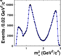
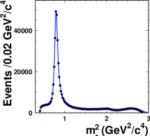
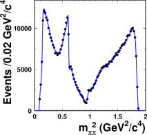
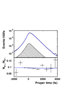
Figure 2: Projection of the unbinned ML fit superimposed on the data for $D^{0}\!\rightarrow\!K^{0}_{S}\,\pi^{+}\pi^{-}$ decays. In (d), the hatched area represents the combinatorial background contribution, and the lower plot shows the ratio of decay-time distributions for events in the $K^{*}(892)^{+}$ and $K^{*}(892)^{-}$ regions, where sensitivity to $(x,y)$ is highest.

For the second fit, $CPV$ is allowed and the $D^{0}$ and $\overline{D}{}^{\,0}$ samples are considered separately. This introduces additional parameters $|q/p|$, ${\rm Arg}(q/p)=\phi$, and $(\bar{a}_{j},\bar{\delta}_{j})$. The fit gives two equivalent solutions, $(x,y,\phi)$ and $(-x,-y,\phi+\pi)$. Aside from this possible sign change, the effect upon $x$ and $y$ is small, and the results for $|q/p|$ and $\phi$ are consistent with no $CPV$. The sets of Dalitz parameters $(a_{r},\delta_{r})$ and $(\bar{a}_{r},\bar{\delta}_{r})$ are consistent with each other, indicating no direct $CPV$. Taking $a_{j}\!=\!\bar{a}_{j}$ and $\delta_{j}\!=\!\bar{\delta}_{j}$ (i.e., no direct $CPV$) and repeating the fit gives $|q/p|=0.95\,^{+0.22}_{-0.20}$ and $\phi=(-2\,^{+10}_{-11})^{\circ}$.

The dominant systematic errors are from the time dependence of the Dalitz plot background, and the effect of the $p_{D^{*}}$ momentum cut used to reject $D^{*}$’s originating from $B$ decays. The default fit includes $\pi\pi$ scalar resonances $\sigma_{1}$ and $\sigma_{2}$; when evaluating systematic errors, the fit is repeated without any $\pi\pi$ scalar resonances using $K$-matrix formalism K-matrix . The influence upon $x$ and $y$ is small and included as a systematic error.

The 95% C.L. contour for $(x,y)$ is plotted in Fig. 3. The contour is obtained from the locus of points where $-2\ln{\cal L}$ rises by 5.99 units from the minimum value; the distance of the points from the origin is subsequently rescaled to include systematic uncertainty. We note that for the $CPV$-allowed case, the reflections of the contours through the origin are also allowed regions.

Figure 3: 95% C.L. contours for $(x,y)$: dotted (solid) is statistical (statistical plus systematic) contour for no $CPV$; dashed-dotted (dashed) is statistical (statistical plus systematic) contour allowing for $CPV$. The point is the best-fit value for no $CPV$.

References

- (1) A. A. Petrov, Int. J. Mod. Phys. A21, 5686 (2006); arXiv:hep-ph/0611361.
- (2) Charge-conjugate modes are included unless noted otherwise.
- (3) S. Bergmann et al., Phys. Lett. B 486, 418 (2000).
- (4) E. M. Aitala et al. (E791), Phys. Rev. Lett. 83, 32 (1999); J. M. Link et al. (FOCUS), Phys. Lett. B 485, 62 (2000); S. E. Csorna et al. (CLEO), Phys. Rev. D 65, 092001 (2002); B. Aubert et al. (BABAR), Phys. Rev. Lett. 91, 121801 (2003).
- (5) M. Staric et al. (Belle), Phys. Rev. Lett. 98, 211803 (2007).
- (6) W.-M. Yao et al. (PDG), Jour. of Phys. G 33, 1 (2006).
- (7) D. M. Asner et al. (CLEO), Phys. Rev. D 72, 012001 (2005); arXiv:hep-ex/0503045 (revised April, 2007).
- (8) A. Poluektov et al. (Belle), Phys. Rev. D 73, 112009 (2006); S. Kopp et al. (CLEO), Phys. Rev. D 63, 092001 (2001).
- (9) L. M. Zhang et al. (Belle), Phys. Rev. Lett. 99, 131803 (2007).
- (10) J. M. Link et al. (FOCUS), Phys. Lett. B 585, 200 (2004); B. Aubert et al. (BABAR), arXiv:hep-ex/0507101 (2005).